Abstract
Usually, data-driven methods require many samples and need to train a specific model for each substation instance. As different substation instances have similar fault features, the number of samples required for model training can be significantly reduced if these features are transferred to the substation instances that lack samples. This paper proposes a fault-line selection (FLS) method based on deep transfer learning for small-current grounded systems to solve the problems of unstable training and low FLS accuracy of data-driven methods in small-sample cases. For this purpose, fine-turning and historical averaging techniques are proposed for use in transfer learning to extract similar fault features from other substation instances and transfer these features to target substation instances that lack samples to improve the accuracy and stability of the model. The results show that the proposed method obtains a much higher FLS accuracy than other methods in small-sample cases; it has a strong generalization ability, low misclassification rate, and excellent application value.
1. Introduction
Small-current grounded systems (SCGSs) are widely used in distribution networks of 66 kV and lower voltage levels, and the number of single-phase grounding faults exceeds 80% of the total number of faults in distribution networks [1,2]. If the neutral of one side of the transformer winding in a substation is ineffectively grounded, the winding, the bus, and the line connected to this bus form an SCGS. Therefore, the substation instances mentioned below refer to a specific SCGS. When a single-phase grounding fault occurs in the SCGS, no prominent fault features can be detected in the fault line, and selecting the fault line from the several lines connected to the bus is called a fault-line selection (FLS) problem. FLS is challenging due to the fault with the random process and inconspicuous fault features.
Traditional FLS methods can be divided into steady-state, transient, and injection methods. Because the steady-state signal is usually weak and susceptible to interference, the steady-state method is less accurate and is difficult to apply in practice [3,4]. The amplitude of transient signals is large, but the duration of the transient process is short and has certain randomness, so the transient method is prone to misjudgment under certain circumstances [5,6]. The injection method injects a specific signal into the system by an additional signal generator and then detects the content of the injected signal in each line and selects the faulty line [7,8]. The additional signal generator increases the cost of FLS significantly, which is not conducive to large-scale applications. Due to the theoretical bottleneck of these methods, it is difficult to fully consider the single-phase grounding fault process with certain randomness. Therefore, their FLS accuracy is generally lower than 70%.
In order to improve the accuracy of FLS, some scholars proposed using data-driven methods such as neural networks to learn fault features from historical data and using these features to select the faulty line [9,10]. This type of method requires many fault samples, the model’s training is very unstable in small-sample cases, and the FLS accuracy is not high enough. To solve the problem of training FLS models with small samples, the paper [11] proposed a generative adversarial network (GAN)-based FLS method to train the classifier using a large number of GAN-generated samples, which alleviates the problem of an insufficient number of samples to some extent. However, the methods proposed in [9,10,11] cannot adapt to different substation instances. It is necessary to build a specific model for each substation instance and then train the model with a large number of samples to obtain a good FLS accuracy. As these methods require many fault samples, they are not conducive to broader application.
Data dependence is one of the toughest problems faced by deep learning [12]. Deep transfer learning exploits similarities in different domains to transfer the features learned from the source domain to the target domain, reducing the number of samples required for model training and achieving better results when solving problems with a lack of samples. Currently, deep transfer learning methods mainly fall into the following four categories: instance-based transfer learning methods [13], mapping-based transfer learning methods [14], adversarial training transfer learning methods [15], and network-based transfer learning methods [16,17]. Network-based transfer learning methods are one of the most common of them, and many pre-designed neural networks can be pre-trained with open-source datasets and then transferred to the desired domain. Among them, models such as AlexNet [18], VGG [19], and ResNet [20] are widely used, and they have achieved excellent results in image classification [21,22].
A necessary condition for deep transfer learning applications is that similarities must exist between the two domains. Similar circuit structures exist in all substation instances; they all satisfy the same physical laws when single-phase grounding faults occur in different instances. If these similar features can be used to build an FLS model that can perform transfer learning between different substation instances, the number of samples required for training can be greatly reduced, and the FLS accuracy can be improved.
In this paper, we consider using the similarity existing in different substation instances to solve the FLS problem using deep transfer learning to extract fault features from other substation instances and transfer these features to the target substation instance to improve the accuracy and stability of small-sample training of the model. The main contributions are as follows.
- An FLS model architecture based on deep transfer learning is proposed. Fine-tuning is used to transfer the fault features extracted from other substation instances to the target instances that lack samples. This will reduce the number of samples required to train the model in the target instance and improve the FLS accuracy.
- The historical averaging technique is proposed for introduction into the transfer learning of the FLS model. It can limit the model parameters to vary widely during the training process. The model can retain the general fault features learned from other substation instances and learn the specific fault features in the target substation instance during transfer training, which improves the transfer effectiveness of the FLS model.
2. Materials and Methods
2.1. Dataset
Fault samples obtained from real SCGSs are used to train and test deep transfer learning models. The SCGS used includes: (1) system A (source domain): a 10 kV bus in a substation; three lines are connected to the bus, and its neutral point is not grounded; (2) system B (target domain): a 10 kV bus in a substation; seven lines are connected to the bus, and its neutral point is grounded through the arc suppression coil.
2.2. Improved Method Based on Deep Transfer Learning
2.2.1. Introduction to Deep Transfer Learning
A schematic diagram of transfer learning is shown in Figure 1. Dataset A with a large number of samples (source domain) and dataset B with only a few samples (target domain) are known to have similar features. Transfer learning enables the model to learn similar features in the source domain and then transfer them to the target domain so that the model can work well in the target domain. The transfer of similar features eliminates the need to train the model from scratch, which significantly improves the training efficiency and model performance.
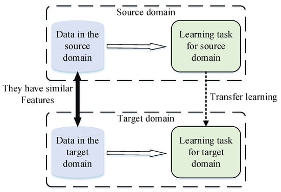
Figure 1.
Schematic diagram of transfer learning.
Currently, deep learning has achieved excellent results in many fields. Transferring the knowledge learned by deep neural networks in the source domain to the target domain has become a popular research direction, called deep transfer learning.
2.2.2. Network-Based Deep Transfer Learning Model
The network-based deep transfer learning method assumes that the feature processing mechanism of the neural network is continuous and progressive, and the first few layers of the network can be regarded as a feature extractor, which can extract general features from the dataset. These features are transferable, i.e., they make the model work well in a target domain similar to the source domain. Therefore, this paper uses fine-tuning to transfer the pre-trained model in the source domain to the target domain for retraining.
The schematic diagram of fine-tuning is shown in Figure 2, which transfers the model parameters that have been trained in the source domain to a new model; then, the new model can be trained in the target domain. During transfer training, the parameters of the first few layers of the network are frozen to retain the general features learned by the model in the source domain, and then the model is trained with data from the target domain. Fine-tuning has the following advantages: (1) it uses a model that has been trained in the source domain and does not need to train a model from scratch; (2) the features from the source domain are preserved in the model, so it can work well when there are only a few samples in the target domain.
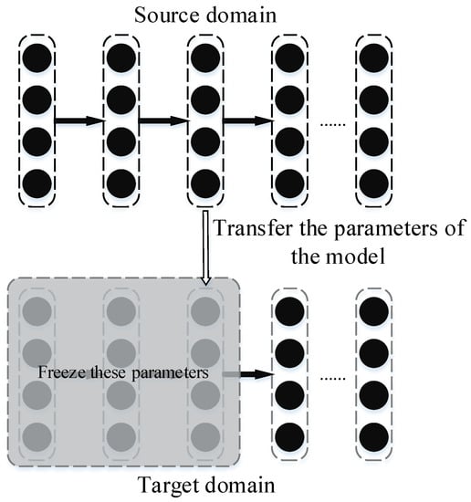
Figure 2.
Schematic diagram of fine-turning.
2.2.3. Improved Model Using Historical Averaging Technique
It was found in the experiment that, when only fine-tuning is used in the transfer learning model, the model effect is not good enough. This may be due to the wide variation in the model’s parameters during training, causing it to forget the general fault features learned in the source domain and thus fall into overfitting.
Therefore, this paper proposes the use of the historical averaging technique to solve the above problems. It refers to adding a historical average term to the model’s loss function, as shown in Equation (1), where represents the model parameters in the neural network at time i. This technique was proposed in [23], where the historical average term can penalize an extensive range of changes in model parameters, guiding the model to find the optimal value near the initial point, which is beneficial for the model to retain the features learned in the source domain.
2.3. FLS Model Based on Deep Transfer Learning
2.3.1. Data Processing of FLS Model
When a fault occurs, the fault samples can be obtained by sampling and processing the data of each line of the substation. The sample format is shown in Equations (2)–(6). represents the data of line n at time i. V, I, P, Q, and denote the bus voltage, line current, active power, reactive power, and power factor, respectively. Their subscripts a, b, and c denote phase a, phase b, and phase c, respectively. represents the bus voltage and the data of one line at time i. x represents a sample. y is a scalar that represents the label of sample x. When sample x corresponds to a faulty line, y is 1; otherwise, it is 0.
Due to differences in operation, the number of lines, and the environment where the lines are installed, there may be order-of-magnitude differences in voltage and current sampling.
The input data processing of the FLS model needs to overcome two main problems: (1) The operating states of different lines in the same substation instance are different, and their operating parameters are quite different. (2) The operating states of different substation instances are different, and their respective operating parameters are quite different. The accumulation of differences caused by the above problems makes the model training very difficult and unable to learn the fault features of the target domain. This paper performs min–max normalization for each physical quantity of different systems, as shown in Equation (7). This processing is beneficial for the model to utilize the fault features of each line and improve the FLS accuracy. takes the voltage, current, active power, reactive power, and power factor of all samples, and then brings them into the formula for calculation. and are the minimum and maximum values of in all samples, respectively.
2.3.2. FLS Model Architecture Based on Deep Transfer Learning
The structure of the FLS model based on deep transfer learning is shown in Figure 3. The classifier of the model consists of multi-layer Bi-LSTM layers and fully connected layers. Bi-LSTM can better utilize the time-series features in the data to improve the model’s ability to select the faulty line [24].
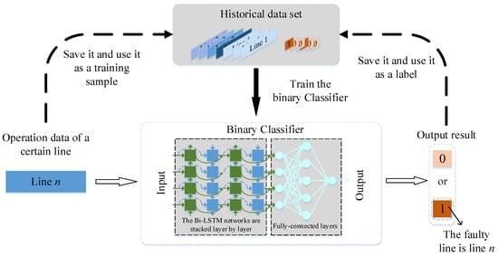
Figure 3.
FLS model architecture based on deep transfer learning.
Although the proposed model can obtain high FLS accuracy, misclassification is inevitable. In the proposed architecture, the real-time fault data and the output results are verified and stored in a historical dataset, and the model is periodically retrained with a new historical dataset to reduce the misspecification of the proposed model.
In this model, the output layer uses the sigmoid activation function, and the loss function is the cross-entropy function, as shown in Equations (8) and (9).
The input data of the FLS model are the operation data of a single line, and the output result is ideally 1 or 0, where 1 indicates that the line is in a fault state, and 0 indicates that the line is in a normal state. In actual operation, the FLS model needs to judge the status of each line in the substation instance separately, and the output result of each line is between 0 and 1. Therefore, it is necessary to select the faulty line according to the output result. There are generally two selection criteria: (1) the maximum value criterion and (2) the threshold value criterion.
(1) Maximum value criterion: The output result of all lines is ; if , it is considered that the fault occurs in line j.
(2) Threshold value criterion: Set the threshold in (0,1). For the output result of all lines, if , it is considered that the fault occurs in line j.
2.4. Training Strategy for FLS Model
2.4.1. One-Step Training Strategy
The one-step training strategy combines samples from the source and target domains into a training set and uses it directly for model training, as shown in Figure 4. The training goal is to minimize the loss of the model to the training set so that the model can learn the features of both domains simultaneously. The samples from system A are introduced into training, which can provide more fault features for the model to avoid the model falling into overfitting and to improve the FLS accuracy of the model. The loss function can be divided into two parts, the source domain (system A) and the target domain (system B), and its mathematical expression is shown in Equation (10).
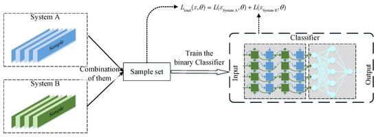
Figure 4.
One-step training strategy for FLS model.
The early stopping method needs to be used during the training process to prevent the model from overlearning the chance features in the data [25]. First, the test loss of the model is recorded at each training epoch, and the model training is terminated early when the test loss shows an increasing trend; then, the weights at this time are used as the final model parameters. The early stopping method can effectively reduce the risk of the model falling into overfitting and the training time, and improves the model’s performance.
The training strategy is simple and effective and can directly transfer the fault features in system A to system B, improving the FLS accuracy in small-sample cases. However, this method trains the data of the source domain and target domain simultaneously, which has certain blindness. The model chooses which features to keep and which features to forget by the gradient generated during training, which is an uncontrollable process.
2.4.2. Two-Step Training Strategy
Although the strategy proposed in Section 2.4.1 is effective, the FLS accuracy of the trained model is still not high enough, due to its inherent flaws. The core reason is that this strategy combines a large number of source domain samples with a few target domain samples for training, which makes the model more inclined to learn features in the source domain rather than those in the target domain.
This paper proposes the two-step training strategy to solve the above problems, as shown in Figure 5. It trains on samples from the source and target domains separately while using fine-tuning and historical averaging techniques to retain the general fault features learned from the source domain, improving the FLS accuracy. The process of the two-step training strategy is as follows:
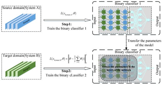
Figure 5.
Two-step training strategy for FLS model.
Step 1: Binary classifier 1 is trained using a large number of samples from the source domain to extract fault features, and its loss function is Equation (11). When the training accuracy of the model satisfies Equation (12), the model training is terminated, where represents the termination accuracy, and the model parameter is at this time. It should be pointed out that parameter represents the fitting degree of the model to the features of the source domain. The improper setting will reduce the effect of transfer learning. In practice, it is generally taken as 70%.
Step 2: Transfer the model parameters of the trained binary classifier 1 to binary classifier 2. Then, the model parameters of the first s layers of the network are frozen, and Equation (13) is used as the loss function to train the binary classifier 2 using the target domain samples to learn the special features of the target domain.
3. Results and Discussion
The proposed method was implemented in Python 3.6 using Keras 2.2.4 and Tensorflow 1.13.1. The model structure used was two-layer Bi-LSTM and four-layer fully connected layers (100-100-50-25). The parameter optimization of the model used the Adam optimizer, and the parameters of the optimizer used the default values.
3.1. The Transfer Learning Process of FLS Model
3.1.1. FLS Model Using One-Step Training Strategy
The FLS model uses the one-step training strategy, trained on 1000 source domain samples and 200 target domain samples, and tested on 500 target domain samples. The training and test results are shown in Figure 6 and Figure 7, and the analysis is as follows.
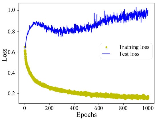
Figure 6.
FLS model loss using a one-step training strategy.
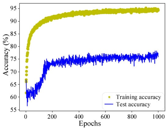
Figure 7.
FLS model accuracy using a one-step training strategy.
The training loss drops rapidly during the 0–50 iterations, while the test loss does not drop but rises rapidly. During 50–200 iterations, as the model fits the samples of system A relatively well, the loss value of this part decreases; then, the samples of system B become the main factor affecting the gradient direction, and the test loss gradually decreases. Eventually, the training and test losses of the model stabilize, and the test accuracy reaches about 75%. The early stopping method is used to terminate the model’s training early at this time, which effectively reduces the overfitting of the model and the invalid training time.
The above results show that the samples of system A in the training set can help the model extract fault features. A small number of system B samples help the model adapt to the difference between system A and system B, significantly improving the FLS accuracy of the model in the target domain. However, due to the blindness of the one-step training strategy, it cannot control which source domain features the model retains, so its accuracy still has room for improvement.
3.1.2. FLS Model Using Two-Step Training Strategy
The model uses the two-step training strategy, and the sample sets used for training and testing are the same as those in Section 3.1.1. In the second step of training, the first three layers of the network are frozen; the termination accuracy is taken as 70%. The analysis is as follows.
The training curve of the FLS model using the two-step training strategy is shown in Figure 8. In the first training step, when the loss value decreases with the training and finally reaches the minimum value, the training is terminated. In the second training step, as the model gradually learns the target domain features, the various losses continue to decrease and eventually stabilize. As shown in Figure 9, the model can achieve about 85% accuracy on the test set. Such high accuracy can be achieved with only a small number of target domain samples, indicating that features in the source domain are well preserved and transferred to the target domain.
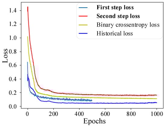
Figure 8.
FLS model loss using a two-step training strategy.
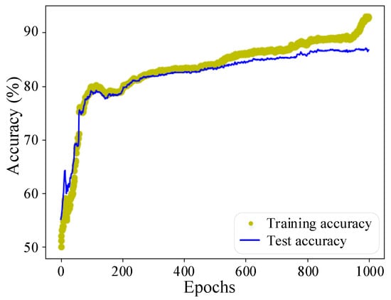
Figure 9.
FLS model accuracy using two-step training strategy.
As the two-step training strategy uses fine-tuning to freeze part of the network layers and uses the historical averaging technique to limit the large changes in model parameters, its fitting effect on the training set is slightly worse than that of the one-step training strategy. Nevertheless, this makes the trained model effectively avoid overfitting, its performance on the test set is better than that of the one-step training strategy, and it has a stronger generalization ability.
3.2. The Effect of Proposed Model on Different Target SCGSs
In order to further verify the transfer learning effect of the proposed model in different target systems, the source domain and target domain in Section 3.1 are exchanged, and then the one-step training strategy (M1) and the two-step training strategy (M2) are trained and tested separately. The results are shown in Table 1.

Table 1.
The training and testing results of the FLS model after exchanging the source and target domains. It should be noted that the test time represents the computation time of the model for one fault in the target domain.
From the time point of view, the training time required by M1 is slightly less than that of M2, while the testing time required by the two methods is about the same. This is because M2 needs to be trained in two steps, and its computational load is relatively large during the training process. Both M1 and M2 perform feedforward computations during the testing process, and their computational load is similar.
From the accuracy of view, M1 has a higher training accuracy than M2, but M2 has a higher test accuracy than M1. This result shows that M2 can better utilize the fault features from the source domain and transfer them into the target domain, thus avoiding the model falling into overfitting.
Furthermore, both methods achieve higher accuracy when the target domain is system A. There are two reasons to explain this result: (1) system A contains fewer lines, and it is easier for the model to identify faulty lines; (2) when system B is used as the source domain, more fault samples of lines can provide more information for model training to improve the model’s performance. Therefore, system instances with more lines and better data quality should be selected as source domains in practical applications.
3.3. Model Comparison
In order to verify the performance of the proposed method in small-sample cases, this section selects the following models and records the accuracies they obtain with different sample sizes. The models proposed in this paper are used in M1–M5. The experimental results are shown in Figure 10, and the analysis is as follows.
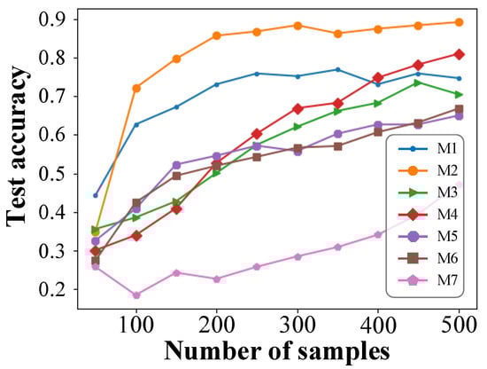
Figure 10.
Test accuracy of each model at different sample sizes.
M1: The one-step training strategy.
M2: The two-step training strategy.
M3: The two-step training strategy without fine-tuning.
M4: The two-step training strategy without historical averaging technique.
M5: The two-step training strategy without fine-tuning and historical averaging techniques.
M6: A deep neural network model based on supervised learning, whose model structure is the same as M1 and only uses the target domain data for supervised training.
M7: Support vector machine model based on supervised learning; its kernel function is RBF and only uses target domain data for supervised training.
- (1)
- When the number of samples is more than 100, the accuracy of M2 is much higher than in other models. Its accuracy can reach about 85% when the sample size is 200, and when the sample size is further increased, the accuracy can even exceed 90%.
- (2)
- Comparing M1 and M2, it can be seen that the two-step training strategy can make the FLS model obtain about 85% accuracy when there are only 200 samples, and its transfer learning effect is significantly better than that of the one-step training strategy.
- (3)
- Comparing M2, M3, M4, and M5, it can be seen that the application of fine-turning and historical averaging techniques can significantly improve the accuracy of the FLS model in small-sample cases. When only one of the two techniques was used, fine-tuning performed slightly better than the historical averaging technique, but they were both significantly better than when neither technique was used.
- (4)
- Comparing M5 and M6 shows that when fine-turning and historical averaging techniques are not used in the two-step training strategy, it is equivalent to a supervised deep neural network model trained only with target domain data. In the two-step training strategy, the model extracts the source domain features in the first step, but if no measures are taken to preserve these features, they may be gradually forgotten by the model with training in the second step.
- (5)
- The effect obtained by M7 is far worse than other models, which indicates that it is difficult for the traditional shallow learning to extract fault features in high-dimensional data.
Table 2 shows each model’s training and test results when only 200 target domain samples are used. The results show that M5 and M6 have the highest training accuracy on the target domain, exceeding 98%. However, they do not make good use of the fault features from the source domain and suffer from severe overfitting; therefore, their test accuracy is low. When using only one of the fine-tuning and historical averaging techniques (M3 and M4), the model’s test accuracy is even lower than when neither technique is used (M5). This suggests that fine-tuning and historical averaging techniques must be applied simultaneously for the FLS model to work well. The training and test time of the shallow learning algorithm (M7) is short, but its training and test accuracy are extremely low. When using the two-step training strategy (M2), the method proposed in this paper can effectively extract fault features from the source domain and select the fault line in the target domain. Therefore, M2 obtains the highest test accuracy in small-sample cases.
Table 2.
Training and testing results for each model when using only 200 target domain samples.
The experimental results show that the proposed method has the best transfer learning effect when using the two-step training strategy, avoiding overfitting and obtaining high FLS accuracy in small-sample cases.
3.4. Effect of Termination Accuracy on FLS Models
The above experiments demonstrate that the performance of the two-step training strategy is better than that of the one-step training strategy. In the two-step training strategy, the termination accuracy indicates how well the model learns the specific features of the source domain, which significantly affects the transfer learning effect of the model. To verify the effect of termination accuracy on the model’s performance, we set different termination accuracies in this section and then record the test accuracy of the model in the target domain. The experimental results are shown in Figure 11 and analyzed as follows.
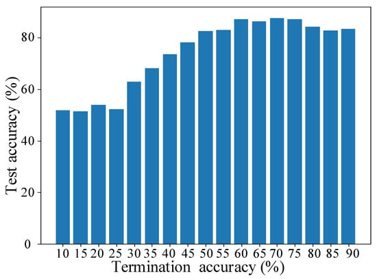
Figure 11.
The effect of termination accuracy on the test accuracy of the model.
As the termination accuracy gradually increases from 10%, the model fits the source domain increasingly well. The features obtained from the source domain are transferred to the target domain, which leads to an increasing trend in the test accuracy of the model. The test accuracy of the model in the source domain reaches its highest value of about 86% when the termination accuracy is around 70%. After that, the test accuracy does not continue to increase as the termination accuracy increases further but decreases slightly.
The results show that the model’s fit to the source domain should not be as high as possible in the two-step training strategy. The higher the termination accuracy that is set, the better the model learns the specific features in the source domain. Overfitting these features can make it difficult to transfer the model to work well in the target domain. Setting the termination accuracy at 70% generally makes model training more stable.
3.5. Operation of FLS Model
Figure 12 illustrates a single-phase grounding fault occurring in system B. When t = 0 s, the bus voltage of the system is abnormal, and the operator successively cuts lines 3, 1, 6, 2, and 7, but the fault is not isolated. About 20 min later, line 5 is cut off, at which time the bus voltage returns to normal, which means that the fault occurs on line 5. The above process cuts off many normal lines, which expands the scope of outages and increases the operating time with faults.
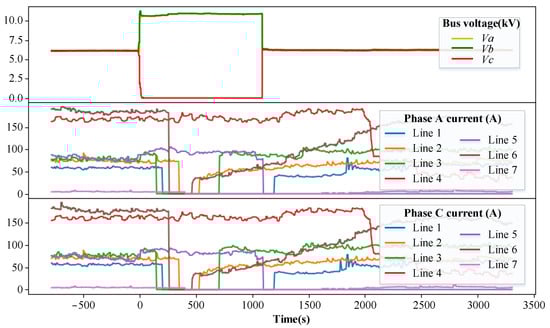
Figure 12.
A single-phase grounding fault in system B.
After pre-training the proposed model in system A and transferring it to system B, the model can be tested with historical data from system B. At t = 0 s, the FLS model detects the fault occurrence and samples the fault data. The sampled data are pre-processed and fed into the FLS model, and then the model output is obtained, as shown in Table 3. According to the maximum value criterion, it can be concluded that the fault occurs on line 5. This FLS process is 0.395 s in total, which can meet the requirement of real-time FLS.
Table 3.
Output of the FLS model for Figure 12.
Figure 13 illustrates a single-phase ground fault occurring in system A. When t = 0 s, the system bus voltage is abnormal. After the operator successfully cuts off lines 2 and 3, the bus voltage returns to normal, which means that the fault occurs on line 3.
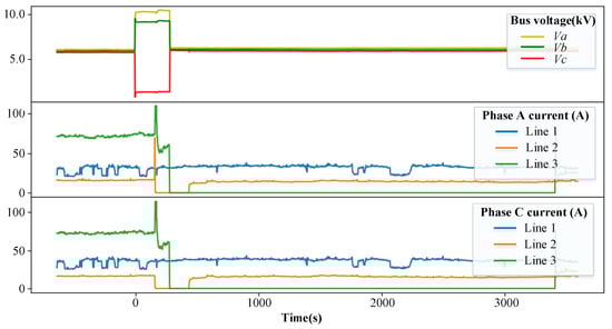
Figure 13.
A single-phase grounded fault in system A.
After pre-training the proposed model in system B and transferring it to system A, the model can be tested with historical data from system A. At t = 0 s, the FLS model detects the fault occurrence and samples the fault data. The sampled data are pre-processed and fed into the FLS model, and then the model output is obtained, as shown in Table 4. According to the maximum value criterion, it can be concluded that the fault occurs on line 3. This FLS process is 0.226 s in total, which can meet the requirement of real-time FLS.
Table 4.
Output of the FLS model for Figure 13.
The computation results show that the proposed method can accurately select the fault line in the target domain after transfer learning, which significantly improves the efficiency of FLS and reduces the negative impact of single-phase grounding faults.
4. Conclusions
This paper proposes a deep-transfer-learning-based fault-line selection method, which solves the problem that data-driven fault-line selection methods are challenging to train in the absence of samples. The proposed method can retain numerous fault features from other instances and transfer these features to the target instance. This greatly reduces the number of samples and the time required for model training in the target instance. In the proposed method, fine-tuning and historical averaging techniques can enhance the model’s training and help the model obtain a fault-line selection model with a better generalization ability in small-sample cases.
The computation results show that the proposed method can maintain high accuracy even when only a few samples are in the target instance. Its training process is stable and relatively simple, and its effect is significantly better than other fault-line selection methods, which have strong practicality.
The proposed method in this paper is affected by the similarity between substation instances, and the transfer effect of the model will be much better between substation instances with higher similarity. However, there is no similarity metric for substation instances to use, which will be a future research direction.
Author Contributions
Conceptualization, X.S. and H.W.; methodology, X.S. and H.W.; software, X.S.; validation, X.S. and H.W.; investigation, X.S. and H.W.; resources, H.W.; writing—original draft preparation, X.S.; writing—review and editing, X.S. and H.W.; visualization, X.S.; supervision, X.S. and H.W. All authors have read and agreed to the published version of the manuscript.
Funding
This research was funded by the National Natural Science Foundation of China (Grant numbers 51967002) and the Guangxi Special Fund for Innovation-Driven Development (Grant no. AA19254034).
Institutional Review Board Statement
Not applicable.
Informed Consent Statement
Not applicable.
Data Availability Statement
Not applicable.
Conflicts of Interest
The authors declare no conflict of interest.
References
- C62.92.4-1991—IEEE Guide for the Application of Neutral Grounding in Electrical Utility Systems, Part IV-Distributio. 1992. Available online: https://ieeexplore.ieee.org/servlet/opac?punumber=2900 (accessed on 21 April 2022).
- Jamali, S.; Bahmanyar, A. A new fault location method for distribution networks using sparse measurements. Int. J. Electr. Power Energy Syst. 2016, 81, 459–468. [Google Scholar] [CrossRef]
- Zhixia, Z.; Xiao, L.; Zailin, P. Fault line detection in neutral point ineffectively grounding power system based on phase-locked loop. IET Gener. Transm. Distrib. 2014, 8, 273–280. [Google Scholar] [CrossRef]
- Cui, T.; Dong, X.; Bo, Z.; Juszczyk, A. Hilbert-Transform-Based Transient/Intermittent Earth Fault Detection in Noneffectively Grounded Distribution Systems. IEEE Trans. Power Deliv. 2010, 25, 143–151. [Google Scholar] [CrossRef]
- Michalik, M.; Okraszewski, T.M. Application of the wavelet transform to backup protection of MV networks-wavelet phase comparison method. In Proceedings of the 2003 IEEE Bologna Power Tech Conference Proceedings, Bologna, Italy, 23–26 June 2003; Volume 2, p. 6. [Google Scholar]
- Zhu, K.; Zhang, P.; Wang, W.; Xu, W. Controlled Closing of PT Delta Winding for Identifying Faulted Lines. IEEE Trans. Power Deliv. 2011, 26, 79–86. [Google Scholar] [CrossRef]
- Fan, S.; Xu, B. Comprehensive application of signal injection method in protection and control of MV distribution system. In Proceedings of the CICED 2010 Proceedings, Nanjing, China, 13–16 September 2010; pp. 1–7. [Google Scholar]
- Niu, L.; Wu, G.; Xu, Z. Single-phase fault line selection in distribution network based on signal injection method. IEEE Access 2021, 99, 21567–21578. [Google Scholar] [CrossRef]
- Yin, H.; Miao, S.; Guo, S.; Han, J.; Wang, Z. Novel method for single-phase grounding fault line selection in distribution network based on S-transform correlation and deep learning. Electr. Power Autom. Equip. 2021, 41, 88–96. [Google Scholar]
- Hao, S.; Zhang, X.; Ma, R.; Wen, H.; An, B.; Li, J. Fault Line Selection Method for Small Current Grounding System Based on Improved GoogLeNet. Power Syst. Technol. 2022, 46, 361–368. [Google Scholar]
- Zhang, L.; Wei, H.; Lyu, Z.; Wei, H.; Li, P. A small-sample faulty line detection method based on generative adversarial networks. Expert Syst. Appl. 2020, 169, 114378. [Google Scholar] [CrossRef]
- Tan, C.; Sun, F.; Kong, T.; Zhang, W.; Yang, C.; Liu, C. A survey on deep transfer learning. In International Conference on Artificial Neural Networks; Springer: Cham, Switzerland, 2018. [Google Scholar]
- Liu, X.; Liu, Z.; Wang, G.; Cai, Z.; Zhang, H. Ensemble transfer learning algorithm. IEEE Access 2017, 6, 2389–2396. [Google Scholar] [CrossRef]
- Gretton, A.; Sejdinovic, D.; Strathmann, H.; Balakrishnan, S.; Pontil, M.; Fukumizu, K.; Sriperumbudur, B.K. Optimal kernel choice for large-scale two-sample tests. Adv. Neural Inf. Process. Syst. 2012, 25. Available online: https://proceedings.neurips.cc/paper/2012/hash/dbe272bab69f8e13f14b405e038deb64-Abstract.html (accessed on 21 April 2022).
- Ganin, Y.; Lempitsky, V. Unsupervised domain adaptation by backpropagation. In Proceedings of the 32nd International Conference on Machine Learning, Lille, France, 6–11 July 2015; pp. 1180–1189. [Google Scholar]
- Chang, H.; Han, J.; Zhong, C.; Snijders, A.M.; Mao, J.H. Unsupervised transfer learning via multi-scale convolutional sparse coding for biomedical applications. IEEE Trans. Pattern Anal. Mach. Intell. 2017, 40, 1182–1194. [Google Scholar] [CrossRef] [PubMed] [Green Version]
- Huang, J.T.; Li, J.; Yu, D.; Deng, L.; Gong, Y. Cross-language knowledge transfer using multilingual deep neural network with shared hidden layers. In Proceedings of the 2013 IEEE International Conference on Acoustics, Speech and Signal Processing, Vancouver, BC, Canada, 26–31 May 2013. [Google Scholar]
- Krizhevsky, A.; Sutskever, I.; Hinton, G.E. Imagenet classification with deep convolutional neural networks. Adv. Neural Inf. Process. Syst. 2012, 25. Available online: https://proceedings.neurips.cc/paper/2012/hash/c399862d3b9d6b76c8436e924a68c45b-Abstract.html (accessed on 21 April 2022). [CrossRef]
- Simonyan, K.; Andrew, Z. Very deep convolutional networks for large-scale image recognition. arXiv Prepr. 2014, arXiv:1409.1556. [Google Scholar]
- He, K.; Zhang, X.; Ren, S.; Sun, J. Deep residual learning for image recognition. In Proceedings of the IEEE Conference on Computer Vision and Pattern Recognition, Las Vegas, NV, USA, 27–30 June 2016; pp. 770–778. [Google Scholar]
- Naushad, R.; Kaur, T.; Ghaderpour, E. Deep Transfer Learning for Land Use and Land Cover Classification: A Comparative Study. Sensors 2021, 21, 8083. [Google Scholar] [CrossRef] [PubMed]
- Elhenawy, M.; Ashqar, H.I.; Masoud, M.; Almannaa, M.H.; Rakotonirainy, A.; Rakha, H.A. Deep Transfer Learning for Vulnerable Road Users Detection using Smartphone Sensors Data. Remote Sens. 2020, 12, 3508. [Google Scholar] [CrossRef]
- Salimans, T.; Goodfellow, I.; Zaremba, W.; Cheung, V.; Radford, A.; Chen, X. Improved techniques for training gans. Adv. Neural Inf. Process. Syst. 2016, 29, 2234–2242. [Google Scholar]
- Su, X.; Wei, H.; Zhang, X.; Gao, W. A Fault-Line Detection Method in Non-Effective Grounding System based on Bidirectional Long-Short Term Memory Network. In Proceedings of the 2021 Power System and Green Energy Conference (PSGEC), Shanghai, China, 20–22 August 2021; pp. 624–628. [Google Scholar] [CrossRef]
- Prechelt, L. Early Stopping—But When? Springer: Berlin/Heidelberg, Germany, 1998. [Google Scholar]
Publisher’s Note: MDPI stays neutral with regard to jurisdictional claims in published maps and institutional affiliations. |
© 2022 by the authors. Licensee MDPI, Basel, Switzerland. This article is an open access article distributed under the terms and conditions of the Creative Commons Attribution (CC BY) license (https://creativecommons.org/licenses/by/4.0/).