Article

Numerical Study on the Long-Term Performance and Load Imbalance Ratio for Medium-Shallow Borehole Heat Exchanger System

1
School of Human Settlements and Civil Engineering, Xi’an Jiaotong University, Xi’an 710049, China
2
Key Laboratory of Coal Resources Exploration and Comprehensive Utilization, Ministry of Natural Resources, Xi’an 710021, China
3
Helmholtz Centre for Environmental Research-UFZ, Permoserstraße 15, 04318 Leipzig, Germany
*
Authors to whom correspondence should be addressed.
Energies 2022, 15(9), 3444; https://doi.org/10.3390/en15093444
Submission received: 2 April 2022 / Revised: 2 May 2022 / Accepted: 5 May 2022 / Published: 9 May 2022
(This article belongs to the Special Issue Energy Conservation in Buildings: Renewable Energy Utilization Method)

Abstract

:
To contribute to the goal of carbon neutralization, the closed-loop borehole heat exchanger system is widely applied to use geothermal energy for building cooling and heating. In this work, a new type of medium-shallow borehole heat exchanger (MSBHE) is proposed, which is coaxial type and has a depth range between 200 m to 500 m. To investigate the long-term performance of MSBHE in the area with unbalanced cooling and heating load of buildings and the sustainable load imbalance ratio under different design parameters, a comprehensive numerical model is established. The results show that the drilling depth significantly influences the sustainable load imbalance ratio of MSBHE. As the drilling depth is increased from 200 m to 500 m, the load imbalance ratio of the MSBHE increases from 20.76% to 60.29%. In contrast, the load imbalance ratio is always kept at the same level with different inlet velocities and operation modes. Furthermore, in a 9-MSBHE array system, the heat exchanger located in the middle of the array has the lowest load imbalance ratio of 48.97%, which is 15.98% lower than the borehole in the edge location. This is caused by the significant influence of the shifted-load phenomenon among MSBHEs in an array system. The findings of the work imply that this newly proposed MSBHE can sustain a notable load imbalance ratio, which is particularly applicable to the areas with a strong imbalance of annual building load.

1. Introduction

In the 21st century, with the rapid development of the global society, the whole world is facing problems such as a sharp increase in energy consumption and increasingly severe environmental pollution [1,2]. Therefore, many countries worldwide have announced corresponding carbon-neutrality policies in recent years. For example, China declared that the carbon peaking and carbon neutrality will be achieved in 2030 and 2060, respectively [3]. The European Union plans to achieve a 55% reduction in greenhouse gas emissions by 2030 [4]. At present, the construction industry consumes about 36% of the global primary energy use and accounts for nearly 40% of the global carbon dioxide emissions [5]. Therefore, using renewable energy to reduce building energy consumption is of great significance for mitigating climate change. Geothermal energy, as a clean energy solution, has the advantages of stability, continuity, and high efficiency [6,7]. With the increasing shortage of fossil energy, the application of geothermal energy in the fields of space heating, bathing, agriculture, and industrial uses has received extensive attention from countries around the world [8].
China has abundant geothermal resources, along with huge demand in the densely populated urban areas and broad developing potential for the market [9,10]. Under the promotion of governments and the efforts of practitioners in related fields, in recent years, geothermal energy utilization technology has been widely used in the field of providing cooling and heating for buildings in China. The primary application forms of geothermal energy include Ground Source Heat Pump (GSHP) coupling with Borehole Heat Exchanger (BHE) and Deep Borehole Heat Exchanger (DBHE) [11].
By the end of 2020, the installed capacity of the geothermal heat pump reached 26,450 MW in China, which is the highest in the world [8]. The application area of shallow geothermal energy and DBHE reached 858 and 13 million m 2 , respectively, in 2019 [8,12]. The deep borehole heat exchanger system extracts the geothermal energy for building heating through a closed metal casing pipe located in a 2000 m∼3000 m depth borehole [13]. This system does not affect groundwater and will not damage the geological environment. However, the initial investment of drilling for the DBHE system is enormous, so it does not currently have broader application worldwide [14,15].
The borehole heat exchanger coupled heat pump also has the following problems in practical application: (1) The ground source heat pump system mainly uses the annual heat storage effect of shallow soil. If the annual cooling and heating load is imbalanced during the long-term operation, the system performance will have obvious degradation [16,17]; (2) The ground source heat pump coupling with borehole heat exchanger system covers a vast area [18]. In urban development, the building density is generally high, so land resources are increasingly scarce. Therefore, the application of ground source heat pump coupled with heat pump is easily restricted by on-site conditions. At present, the imbalance of cooling and heating load of the ground source heat pump system is usually alleviated by adding auxiliary systems. However, this is bound to increase the initial investment, operation cost, and control complexity of the system [19]. Therefore, the analysis of soil thermal balance of a ground source heat pump system in long-term operation is crucial.
Nowadays, three methods are mostly adopted to execute the BHE-related research: field monitoring test, analytical solution analysis, and numerical simulation. However, only a few studies [20,21,22,23] give the monitoring data of long-term operation of ground source heat pump system and only include single BHE or small-scale BHE system. In recent years, some scholars have studied large-scale [24] and super large-scale [25] BHE systems. However, they only have short-term operation data. Compared with the research on actual monitoring data, the analytical solution and numerical solution make it more economical and convenient [26,27]. The commonly used analytical solution models can be roughly divided into line source [28], cylindrical source [29] and finite line source (FLS) models [30,31]. Philippe et al. [32] compared the results among the infinite line source, infinite cylindrical source, and FLS models to determine their validity domains. In order to predict the temperature of circulating fluid, Li et al. [33] proposed a composite medium line source model. Zhang et al. [28] proposed a transient quasi three-dimensional line source model to calculate the temperature response in the whole life cycle and used the model to analyze the temperature field distribution of heat transfer fluid and soil. However, the analytical solution model adopts many assumptions in the calculation process, which has limitations in time and space [26]. The numerical solution has fewer assumptions and is more practical [34]. The commonly used numerical solution models include the finite difference method [35,36], finite volume method, and finite element method [37]. Many researchers also use commercial software for calculation and analysis, such as FEFLOW [38,39], COMSOL [40], and FLUENT [41].
Based on the above three methods, many scholars use the load imbalance ratio to analyze the ground source heat pump system’s cooling and heating load imbalance feature. Yang et al. [16] pointed out that the underground thermal imbalance will become more severe when the ratio of heat rejected into the soil and heat abstracted from the soil increases. Qian and Wang [17] also reached a similar conclusion: the accumulation of heat in the soil will reduce the system performance, and the intermittent operation mode can balance the accumulation of heating load and cooling load to improve the system performance significantly. Luo et al. [42] analyzed the measured data of an office building and found that the cooling energy efficiency of the GSHP system is gradually improved, and the heating energy efficiency is progressively reduced because the building’s heating load is much greater than the cooling load. These studies show that the cooling and heating load imbalance will harm the system’s performance. However, most of the existing studies concerning load imbalance ratio are based on short-term simulations [16], and the depth of the borehole heat exchanger is basically within 200 m [16,17].
Generally, it is necessary to maintain load balance for the conventional shallow borehole heat exchanger. However, the imbalance of annual building load is widely existing in many areas. This paper proposes a medium-shallow borehole heat exchanger (MSBHE), which breaks the limitation that the shallow borehole heat exchanger is no more than 200 m in depth. When the drilling depth is appropriately increased, the heating capacity of the MSBHE will be stronger than the cooling capacity [43], and a load imbalance is allowed in the whole system. This MSBHE system can avoid the decline of system performance caused by the load imbalance of the conventional shallow ground source heat pump system and make up for the disadvantage of the deep borehole heat exchanger by providing cooling for buildings. When applying the MSBHE system to building cooling and heating, the following questions need to be answered: Can the MSBHE operate stably for the long term under an imbalanced load? How does the sustainable load imbalance ratio of MSBHE change under different design parameters?
In this paper, OGS-TESPy software is used to construct the MSBHE array model according to the actual geological parameters of Xi’an, China, and then the scientific problems raised above are studied through detailed numerical simulation. The long-term numerical simulation confirmed that MSBHE can operate for 15 years in the presence of load imbalance. Then, the changes of load imbalance ratio of a single MSBHE and typical MSBHEs in the MSBHE array are analyzed in detail. The research of this paper will provide a new scheme for the utilization of geothermal energy and the borehole heat exchanger can be utilized in broader areas.

2. Methodology

This section presents the model framework and numerical methods for simulating MSBHE arrays.

2.1. OpenGeoSys

There are several types of conventional shallow borehole heat exchangers, including single U-shape pipe (1U), double U-shape pipe (2U), and coaxial pipe. As for the medium-shallow borehole heat exchanger proposed in this research, the coaxial pipe is selected because of its higher pressure endurance and convenience in construction. Based on the previous research, a coaxial pipe with an annular inlet (CXA) obtains better performance in heat exchanger capacity than a coaxial pipe with a centered inlet (CXC). Thus, the simulation carried out in this study is aimed at the medium-shallow borehole heat exchanger with CXA type. In order to investigate the two key scientific questions raised above, it is necessary to establish a numerical model of the MSBHE array with geothermal gradient and hydraulic interaction. Furthermore, OpenGeoSys (OGS) software will be the preferred numerical simulation software for this study because the calculation speed of long-term operation simulation is maintained at an acceptable level [44].
As the core mechanism of the H E A T _ T R A N S P O R T _ B H E module [45] in OGS software, Dual-continuum Finite Element Method (DC-FEM) divides the model domain into two parts: one is a simplified 1D linear finite element mesh for the borehole part (including MSBHE and surrounding grout), the other consists of discretized 3D prism cells for the soil part. The coupling between the borehole part and soil part depends on the Robin-type boundary condition of heat flux. Convective and conduction heat balance equations are solved in the 3D model domain, reflecting heat dissipation from the subsurface. For the interested reader, the governing equations of heat conduction and convection deployed in the OpenGeoSys software can be found in previous publications [44,46]. Compared with the analytical solution, OGS can describe complex boundary conditions and consider complex geological conditions successfully, and compared with other mature commercial software, such as FLUENT and COMSOL, the number of meshes can be greatly reduced by neglecting the diameter and thickness of the tube in millimeters.

2.2. Coupling OpenGeoSys and TESPy

In practical engineering applications, multiple borehole heat exchangers often operate at the same time to meet the load requirements of buildings. Therefore, the thermal interaction between MSBHEs needs to be considered to accurately calculate the heating and cooling capacity of MSBHE. The software Thermal Engineering System in Python (TESPy) [47] can be used to calculate the pressure, mass flow, and fluid enthalpy at each network connection in the MSBHE network. TESPy is to solve the control equation of mass and energy balance through Newton–Raphson iteration, in which the properties of circulating fluid in MSBHE pipe network are dynamically updated through CoolProp library [48].
In OpenGeoSys, we embed the Python interface library pybind11 [49], which can realize the mutual transmission of calculation results between OpenGeoSys and TESPy. Within every time step and each iteration, the outflow temperature from each MSBHE is simulated by OpenGeoSys and then transferred to TESPy via the Python interface. The circulation temperature and the current hydraulic state are transmitted to TESPy for pipe network calculation. TESPy will calculate the current inflow temperature of each MSBHE and their flow rate, which satisfies the thermal load imposed on the pipe network. These computed data are then transferred back to OpenGeoSys for the next iteration. The convergence will be achieved when the norm difference from the last two iteration results is smaller than a preset tolerance of 10 6 for both types of software. The detailed calculation logic can be found on TESPy’s website [50].

2.3. Load Imbalance Ratio

In this work, the load imbalance ratio (LIR) is proposed to assess the level of the difference between the cumulative heating and cooling load imposed on the MSBHE. It is defined as:
L I R = Q A H I Q A C S max ( Q A H I ,   Q A C S ) × 100 %
where Q A H I is the accumulated heat imposed on the MSBHE during the heating season and Q A C S is the accumulated cooling supplied by the MSBHE during the cooling season. A positive LIR indicates that the imposed heating load is greater than the cooling load. In contrast, a negative LIR indicates that the imposed heating load is less than the cooling load.

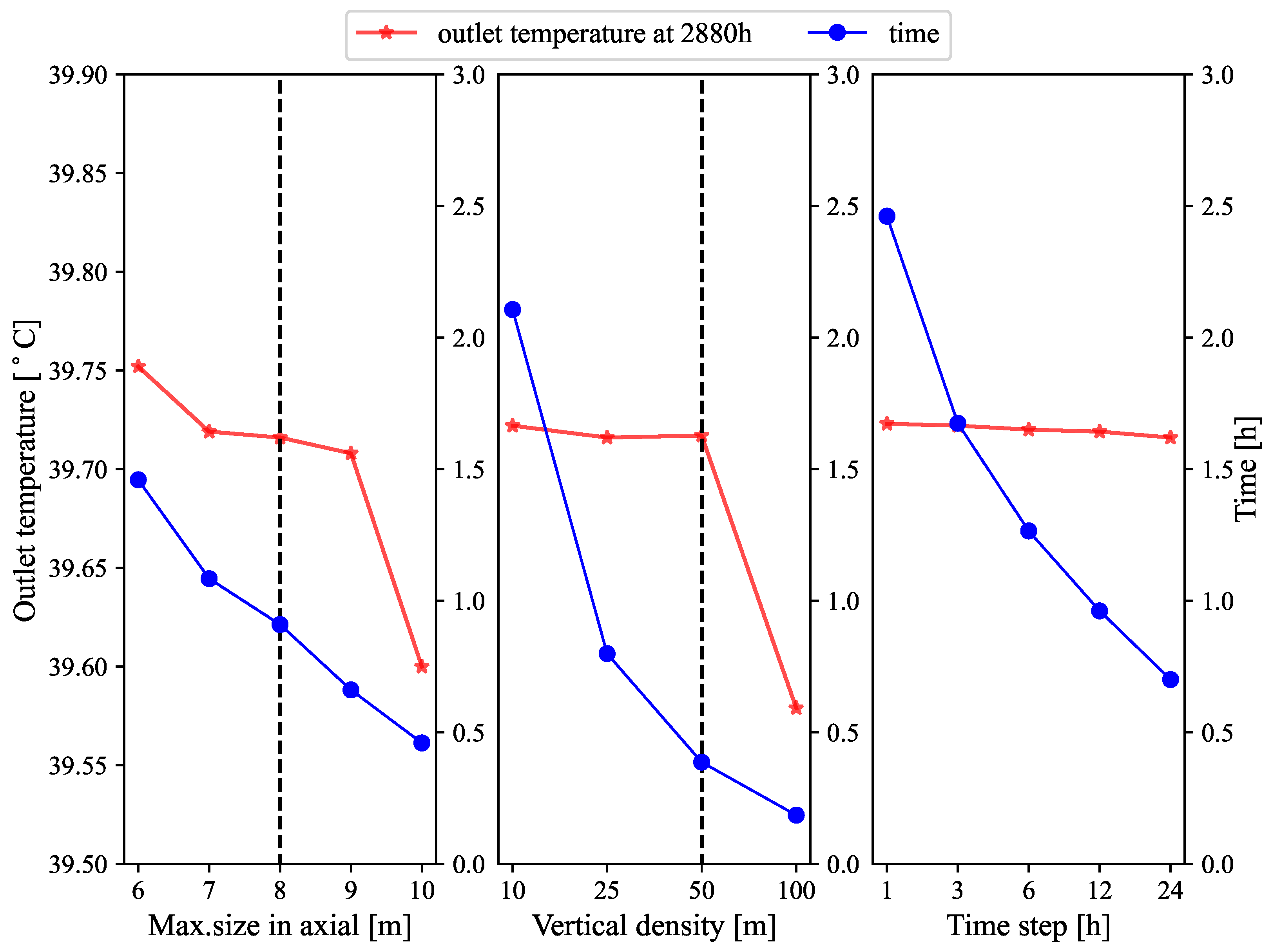
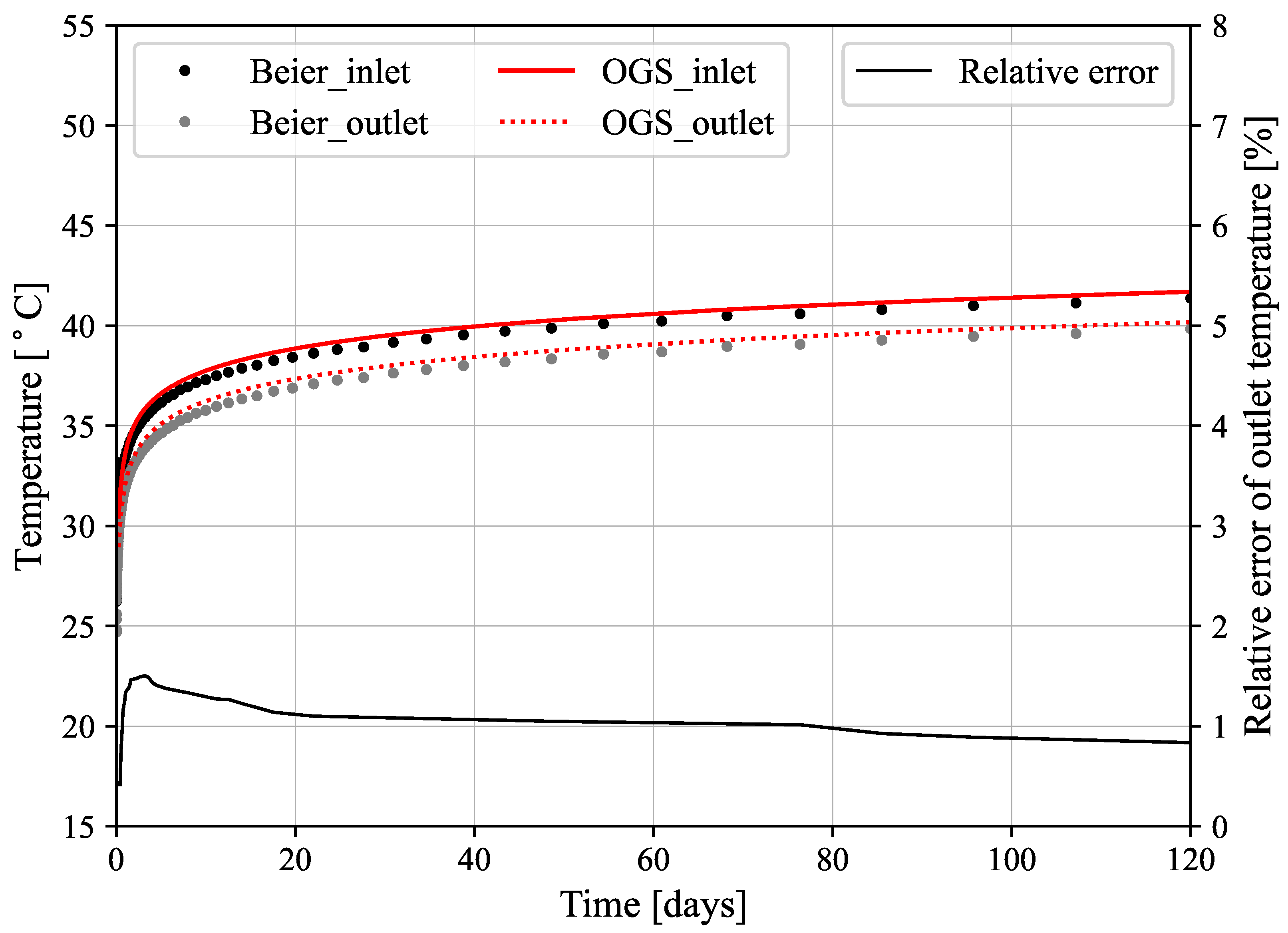
3. Model Configuration and Verification

The model in this study is set up according to the geological conditions of the Xi’an area [13]. At the top of the model domain, the monthly mean ambient air temperature of Xi’an is imposed as a Dirichlet boundary condition [51]. The lateral surface of the model domain is set as the no-heat-flux boundary condition. The bottom of the model domain is also set as Neumann boundary condition with the standard geothermal heat flux in the Xi’an area. The depth of the fluctuated temperature layer is about 20 m [52]. The initial soil temperature of 17.5 ° C will change within this range with the local climate. Below the fluctuated temperature layer, the soil temperature will not be affected by local climate change and will increase with depth controlled by the geothermal gradient. Table 1 shows the detailed parameters of the MSBHE system.
In order to avoid the interference of the thermal plume generated during the long-term operation of MSBHE on the model boundary, the domain size is selected as 100 × 100 × 555 m. Considering the calculation cost and accuracy, it is necessary to reasonably select the grid size and time step of the model. Therefore, a series of axial and vertical grid density and time independence tests were carried out. The test results are shown in Figure 1. The results show that the changes of axial and vertical dimensions have a certain impact on the outlet temperature, and the larger grid size will produce inaccurate temperature results. Therefore, the maximum size of the axial element is set to 8 m and the vertical grid density is set to 50 m. The change of the time step has little effect on the calculation results. In this study, the time step gradually increases from 1 h to 24 h.
The OGS-TESPy model has been verified and validated by the analytical model, numerical model, and measured data [44,53,54]. This paper verifies the OpenGeoSys model with Beier’s analytical model, which has the geothermal gradient considered [55]. The verification results (see Figure 2) show that the inlet and outlet temperature of circulating fluid calculated by OpenGeoSys matches well with the calculated results of Beier’s analytical solution model. In the early stage of simulation, the system has not reached the steady state, so the relative error of the outlet temperature of the two models reaches the maximum value of 1.5%. Then, the relative error between the two models decreases gradually. The validation results show that the MSBHE model has sufficient accuracy and can be used to study long-term performance.

4. Results

4.1. Single MSBHE

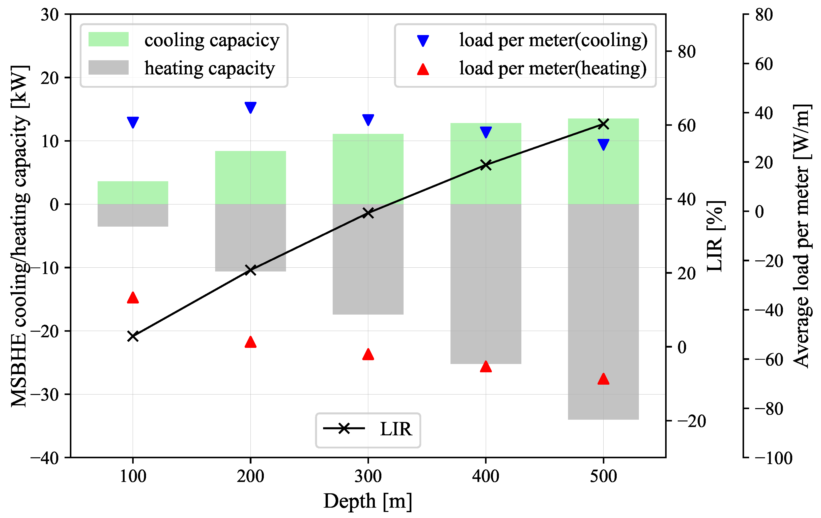
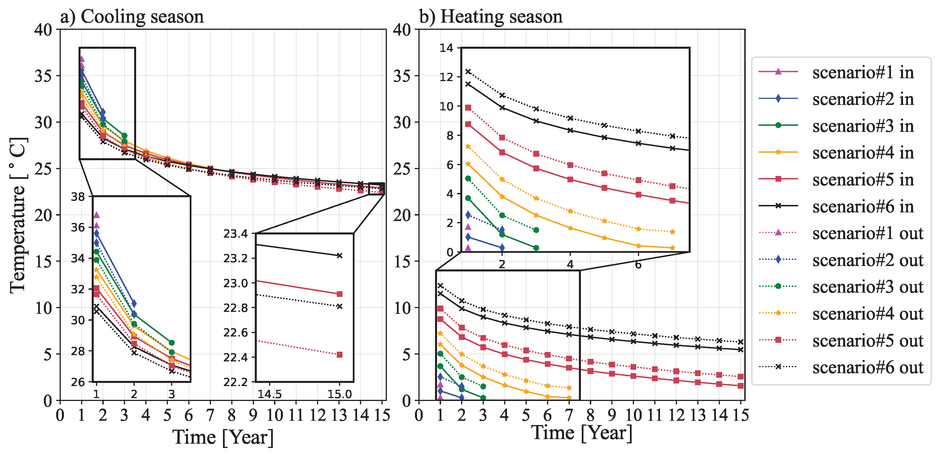
4.1.1. Influence of Depth

According to the domestic technical standard [56], the maximum outlet temperature of the BHE should be lower than 33 ° C in summer, and the minimum outlet temperature of the BHE without antifreeze should be higher than 4 ° C in winter. In order to meet the threshold of the MSBHE’s inlet and outlet temperature, the values of Q A H I and Q A C S are restricted in a specific range. Therefore, by changing the value of the load per meter of the MSBHE in the cooling and heating season, then performing multiple sets of numerical simulations, the range of Q A H I and Q A C S can be found. According to this range, the maximum LIR can be calculated.
To find the range of Q A H I and Q A C S , different scenarios were set (see Table 2), in which the related parameters of the MSBHE are the same as Table 1. Under scenario 1 and 2, the accumulated cool supplied by the MSBHE is equal, and under scenario 1 and 3, the accumulated heat imposed on the MSBHE is the same. Figure 3 shows the evolution of the outlet temperature of MSBHE under the above three scenarios for 15 years. It can be seen that the outlet temperature of the MSBHE showed a decreasing trend, which is because the heat absorbed by the MSBHE is greater than the heat rejected, resulting in lower soil temperature. The maximum outlet temperature of MSBHE in scenario 1 and 2 is equal, both of which are 32.97 ° C, which meets the requirements for summer water temperature. The maximum outlet temperature in scenario 3 reaches 33.27 ° C, which does not meet the requirements. Because the maximum outlet temperature of the MSBHE increases with the increase of cooling load, to meet the requirement of 33 ° C threshold, the load per meter of the MSBHE in the cooling season should not be greater than 27 W. This means that the cool supplied by the MSBHE ( Q A C S ) is no more than 27 × 500 × 3600 × 24 × 120 × 15 = 2.10 × 10 12 J. The lowest outlet temperature for scenarios 1, 2, and 3 are 4.02 ° C, 3.69 ° C, and 4.06 ° C, respectively. Comparing scenario 1 and 2, under the same cooling load, the increase in heating load will decrease the minimum outlet temperature of the MSBHE. Compared with scenario 1 and 3, since the increase of summer load is conducive to the recovery of soil temperature, the lowest outlet temperature of MSBHE in scenario 3 is higher. To sum up, the heating load of MSBHE shall not exceed 68 W/m, that is, Q A H I is is no more than 68 × 500 × 3600 × 24 × 120 × 15 = 5.29 × 10 12 J. After obtaining the range of Q A C S and Q A H I , the maximum load imbalance ratio (LIR) can be calculated, which is 60.29% under the condition of meeting the long-term stable operation of MSBHE during 15 years.
Figure 4 illustrates the maximum heating and cooling capacity of MSBHE under the temperature threshold at different depths and the corresponding load imbalance ratio. In order to compare with the conventional shallow BHE, a working condition with a depth of 100 m is set. According to Figure 4, it can be found that with the increase of drilling depth of MSBHE, the cooling and heating capacity of MSBHE will increase. When the drilling depth increases from 100 m to 500 m, the cooling capacity of the MSBHE increases from 3.6 kW to 13.5 kW, and the heating capacity increases from 3.5 kW to 34.0 kW. The cooling capacity of the MSBHE increased by 3.75 times, and the heating capacity increased by 9.71 times, which is almost 2.50 times that of the former. As the drilling depth increases, the total heat transfer of the MSBHE in the cooling season increases. However, the changing trend of the load per meter of the MSBHE is not the same, first having an increment from 36 W/m (100 m) to 42 W/m (200 m), then gradually decreasing to 27 W/m (500 m). On the contrary, the changing trend of the load per meter of the MSBHE in the heating season is the same as the total heat transfer, both increasing gradually with the increase of depth, and the load per meter increasing from 34 W/m (100 m) to 67 W/m (500 m). It can be seen from Figure 4 that the load imbalance ratio of borehole heat exchanger (100 m) in the category of conventional shallow GSHP is basically 0%. However, the load imbalance rate of MSBHE increases rapidly with the increase of depth. When the depth of MSBHE increases from 200 m to 500 m, the load imbalance ratio increases from 20.76% to 60.29%.

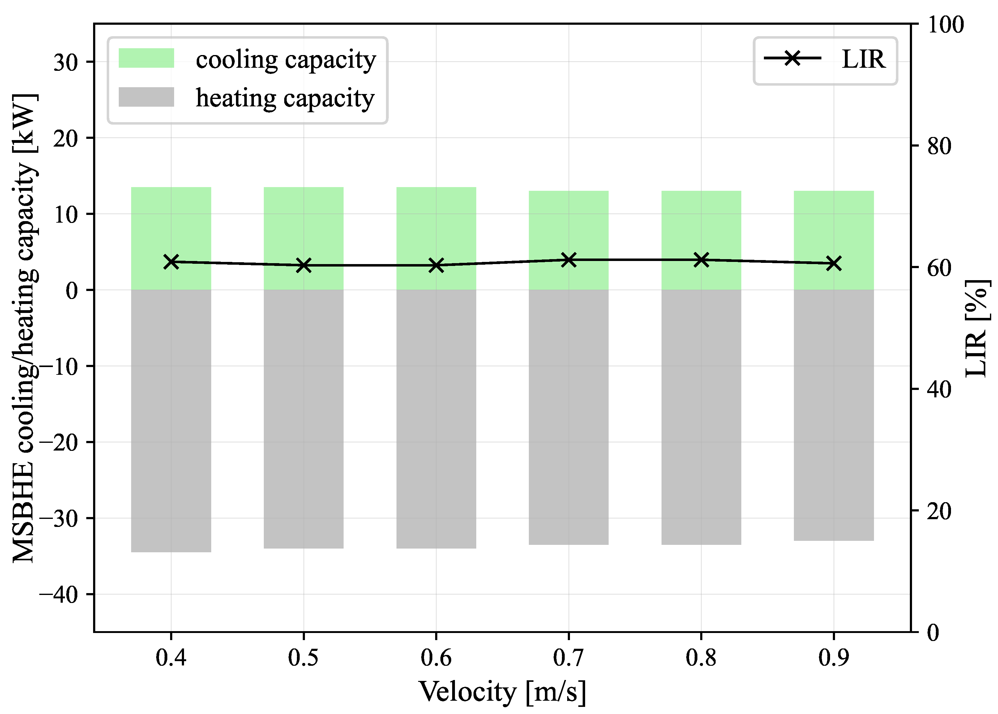
4.1.2. Influence of the Flow Rate

As shown in Figure 5, the cooling capacity, heating capacity, and load imbalance ratio of MSBHE did not change obviously with a change of the inlet flow rate. When the MSBHE’s inlet flow rate is increased from 0.4 m/s to 0.9 m/s, the cooling capacity of the MSBHE is reduced from 13.5 kW to 13.0 kW. At the same time, the heating capacity of the MSBHE is reduced from 34.5 kW to 33.0 kW. Therefore, the load imbalance ratio of MSBHE can be calculated, which is always maintained at about 60%. When the inlet flow velocity of the MSBHE is 0.4 m/s, the LIR is 60.87%, which is the maximum. When the inlet flow velocity is 0.5 m/s and 0.6 m/s, the LIR is 60.29%, which is the minimum. Furthermore, the difference between the maximum and minimum is only 0.58%.

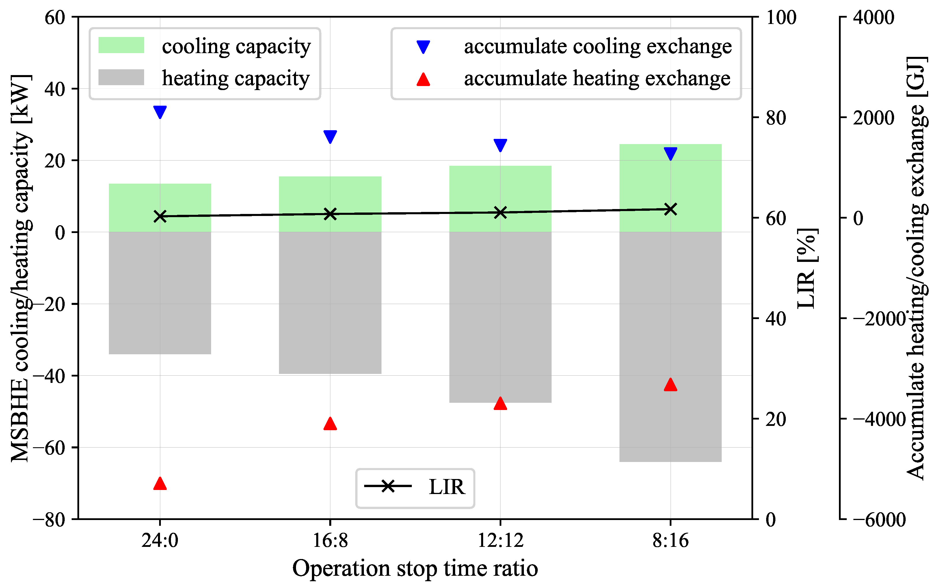
4.1.3. Influence of Operation Mode
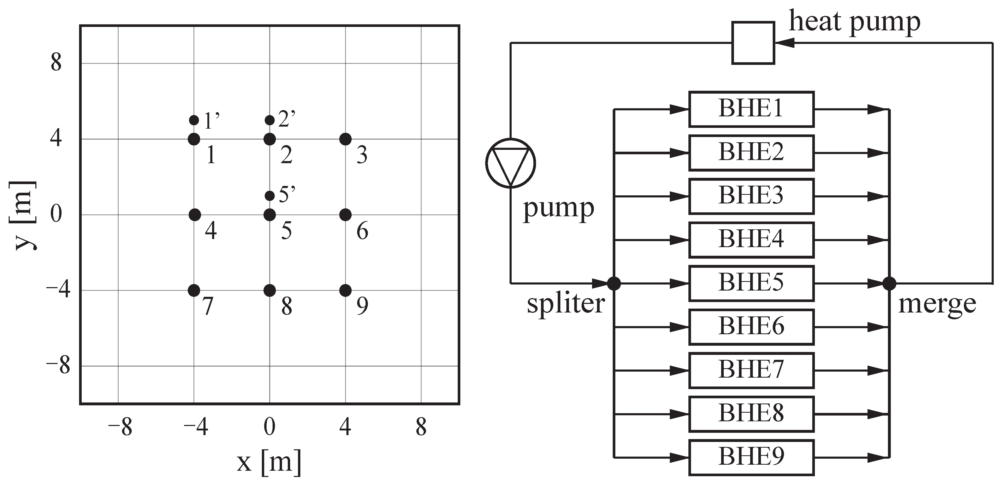
Usually, the operation time of the ground source heat pump system may be different in different types of buildings. Therefore, four scenarios with the different daily loads for MSBHE are set in this study, and the long-term simulations for 15 years are carried out. Figure 6 shows the maximum cooling and heating capacity of MSBHE and load imbalance ratio under different scenarios. It can be seen from Figure 6 that when the daily operation time of the MSBHE is sequentially reduced from 24 h to 8 h, the cooling capacity of the MSBHE is sequentially increased from 13.5 kW to 24.5 kW. The MSBHE will reject heat into the soil during the cooling season, which will increase the soil temperature. However, the higher temperature soil will be unfavorable for the MSBHE to continue to reject heat into the subsurface. When the MSBHE runs intermittently, the soil temperature around the MSBHE will recover in the intermittent period so that the heat exchange efficiency will be higher. The longer the MSBHE stops running, the better the soil temperature recovery and the stronger the cooling capacity of the MSBHE. The trend of MSBHE’s heating capacity is the same as the cooling capacity, increasing from 33.5 kW to 63.5 kW. When the MSBHE stops operating during the heating season, the Earth’s heat flow and solar radiation will increase the soil temperature, which is beneficial for MSBHE to extract heat from the soil. Although the cooling and heating capacity of the MSBHE increases with the increase of the intermittent time, the accumulated cooling and heating exchange of the MSBHE gradually decreases during the 15-year life cycle. The reduction of MSBHE operation time has a more significant impact on the accumulated cooling and heating exchange than the increase of the cooling and heating capacity. When the intermittent operation time changed, the cooling capacity, heating capacity, and the accumulated heat exchange of the MSBHE changed significantly. However, the LIR has barely changed, only slightly increasing from 60.29% to 61.72%, which can be explained by better soil recovery with longer intervals.

4.2. MSBHE Array

In practical engineering applications, to meet the load requirements of buildings, the GSHP system is usually composed of dozens or even hundreds of heat exchangers. Therefore, the model composed of one MSBHE is extended to the MSBHE array model with nine heat exchangers to study the change of LIR in the MSBHE array. The arrangement of the MSBHE array is shown in Figure 7. The spacing between adjacent MSBHE is 4 m, which complies with the requirement of a minimum spacing of 3 to 6 m between BHEs in China [56], and other relevant parameters remain unchanged. According to the research of Chen et al. [53], the phenomenon of heating and cooling load accumulation will occur in the long-term operation of the BHE array, which will lead to the decline of the heat exchange performance of the BHE located in the middle of the array. In other words, the inlet and outlet temperature of MSBHE #5, which is located in the center, may exceed the threshold when carrying the same cooling and heating load as the single MSBHE model. Therefore, six different scenarios (numbered from #1 to #6) are set. The average cooling and heating load of the MSBHE in each scenario is 100%, 90%, 80%, 70%, 60%, and 50% of the maximum cooling and heating load under the single MSBHE model. Then, a 15-year long-term simulation of all six scenarios was performed to study the behavior of the MSBHE array.

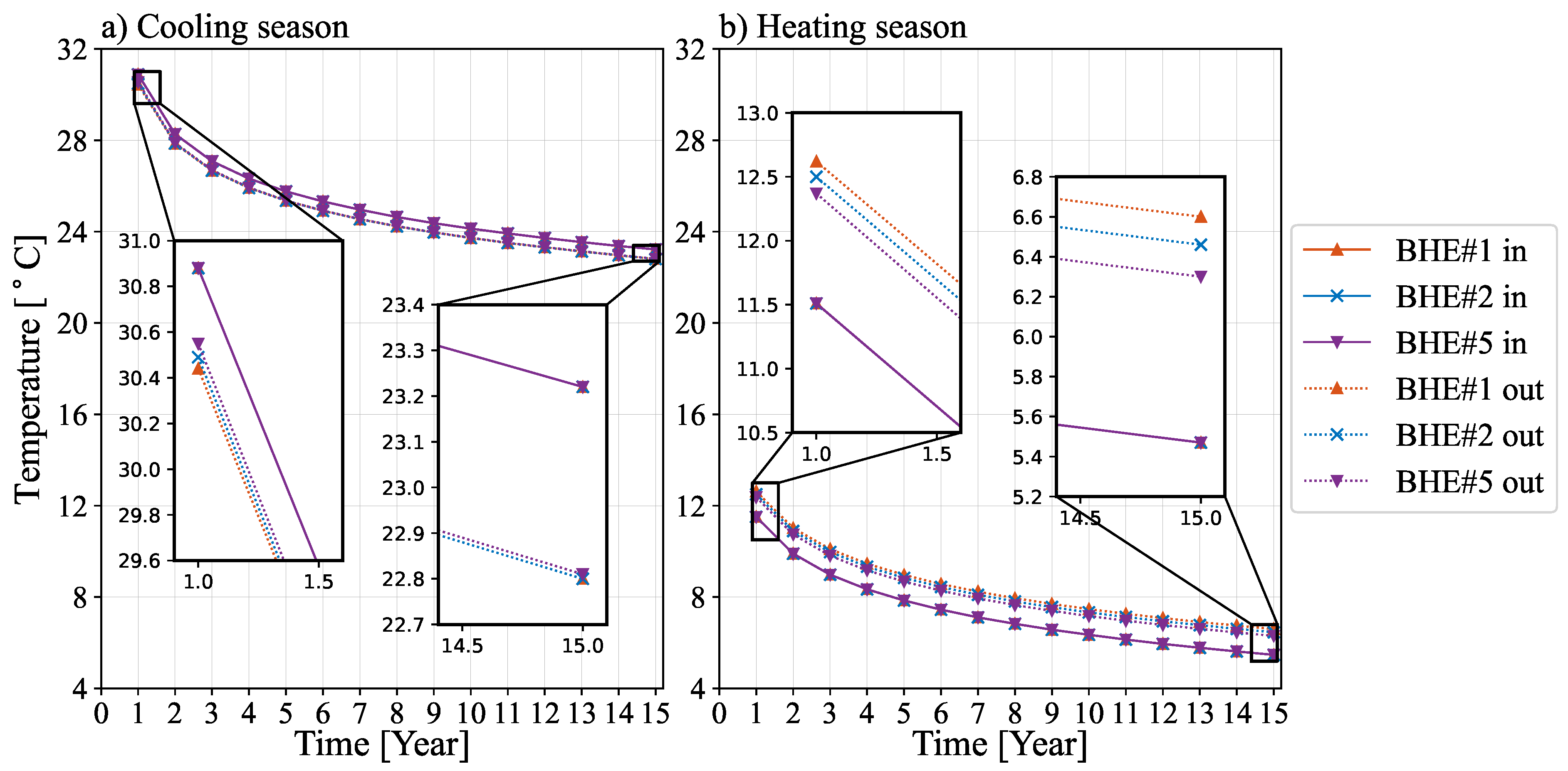
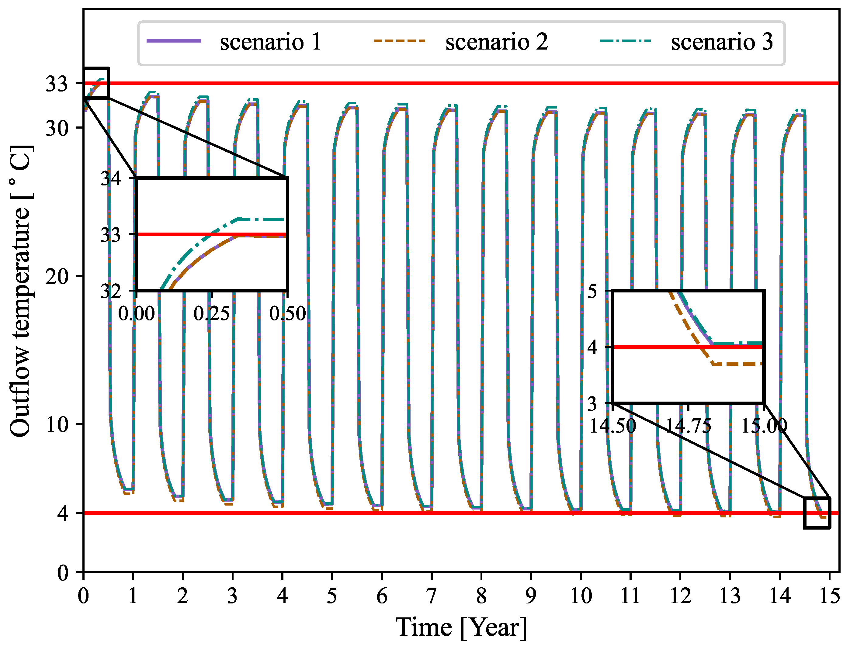
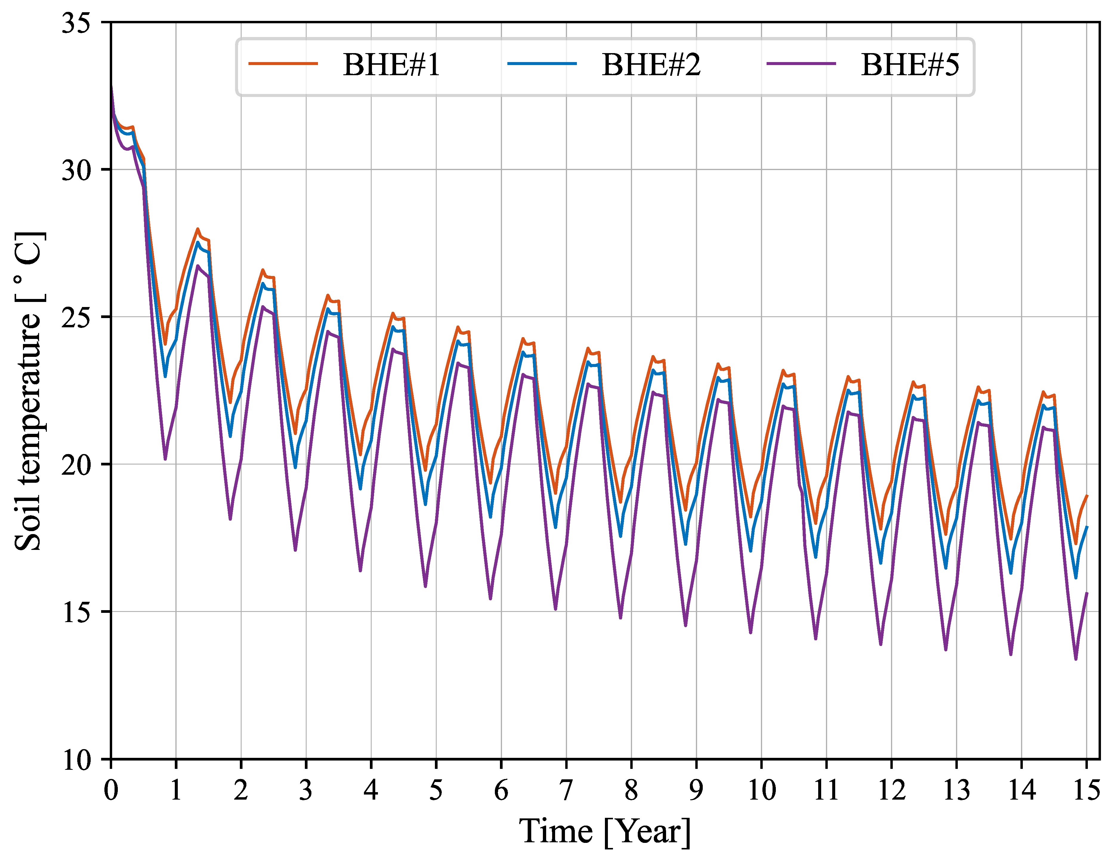
4.2.1. Evolution of Temperature

Figure 8 shows the evolution of inlet and outlet temperature of MSBHE #5 at the end of cooling and heating season under the above six scenarios. Only the inlet and outlet temperature of MSBHE #5 in scenario #6 meets the requirements of the temperature threshold. In other words, the average cooling and heating load of MSBHE in a 3 × 3 system is only 50% of that of a single MSBHE system, which means the heat exchange performance of the MSBHE has decreased significantly. Because the arrangement of the 3 × 3 MSBHE system is symmetrical, MSBHE #1, #2, and #5 are selected as representatives for analysis. Figure 9a,b show the changes of the inlet and outlet temperature of the three selected MSBHEs at the end of the cooling and heating season under scenario#6. Due to the existence of the water separator, the inlet temperature of the MSBHEs is always the same, while the outlet temperature is different. During the cooling period, the outlet temperature of MSBHE #5 is slightly higher, followed by MSBHE #2, and the lowest is MSBHE #1, but they are nearly equal. During the heating period, the difference in outlet temperature between MSBHE #1, #2, and #5 is noticeable, and the maximum temperature difference reaches 0.3 ° C. Furthermore, the outlet temperature of MSBHE #5 is the highest, and the outlet temperature of MSBHE #1 is the lowest, just opposite the cooling season.
Figure 10 shows the evolution of soil temperature at a depth of 505 m and 1 m away from the selected MSBHEs at the end of cooling, heating, and recovery season under scenario #6. The specific positions are shown in the three points 1 , 2 , and 5 in Figure 7. The soil temperature showed a downward trend as a whole. However, the interesting point is that the soil temperature decreases after the first refrigeration period, which means that the temperature of the circulating fluid when reaching the bottom of the MSBHE is lower than that of the surrounding soil. The circulating fluid absorbs heat from the soil, resulting in decreased soil temperature. As the circulating fluid returns to the ground, the heat absorbed will be released to the subsurface. This process is not conducive for the MSBHE to provide cooling to the building. It is also consistent with the result that the cooling capacity per meter decreases when the drilling depth of the MSBHE increases, as shown in Figure 4.
It can be seen that the soil temperature near the centered MSBHE is the lowest, indicating an apparent cold accumulation. The heat imposed on the MSBHE array is far greater than the cooling load so that a decrease in soil temperature occurs. Moreover, the soil at the center of the MSBHE array gets less heat supplement so that the temperature will be lower. After the cooling season, the soil temperature will decrease in the recovery period, and the soil near MSBHE #5 will drop more. After the first recovery period, the soil temperature of MSBHE #1, #2, and #5 decreased by 1.06 ° C, 1.15 ° C, and 1.38 ° C, respectively. After that, the range of soil temperature drop in the recovery period after the cooling season is significantly reduced. In contrast, the soil temperature in the recovery period after the heating season will rise due to the heat recovery of the subsurface. Taking the MSBHE #5 as an example, the soil temperature increased by 1.75 ° C in the first year and 2.22 ° C in the last year.

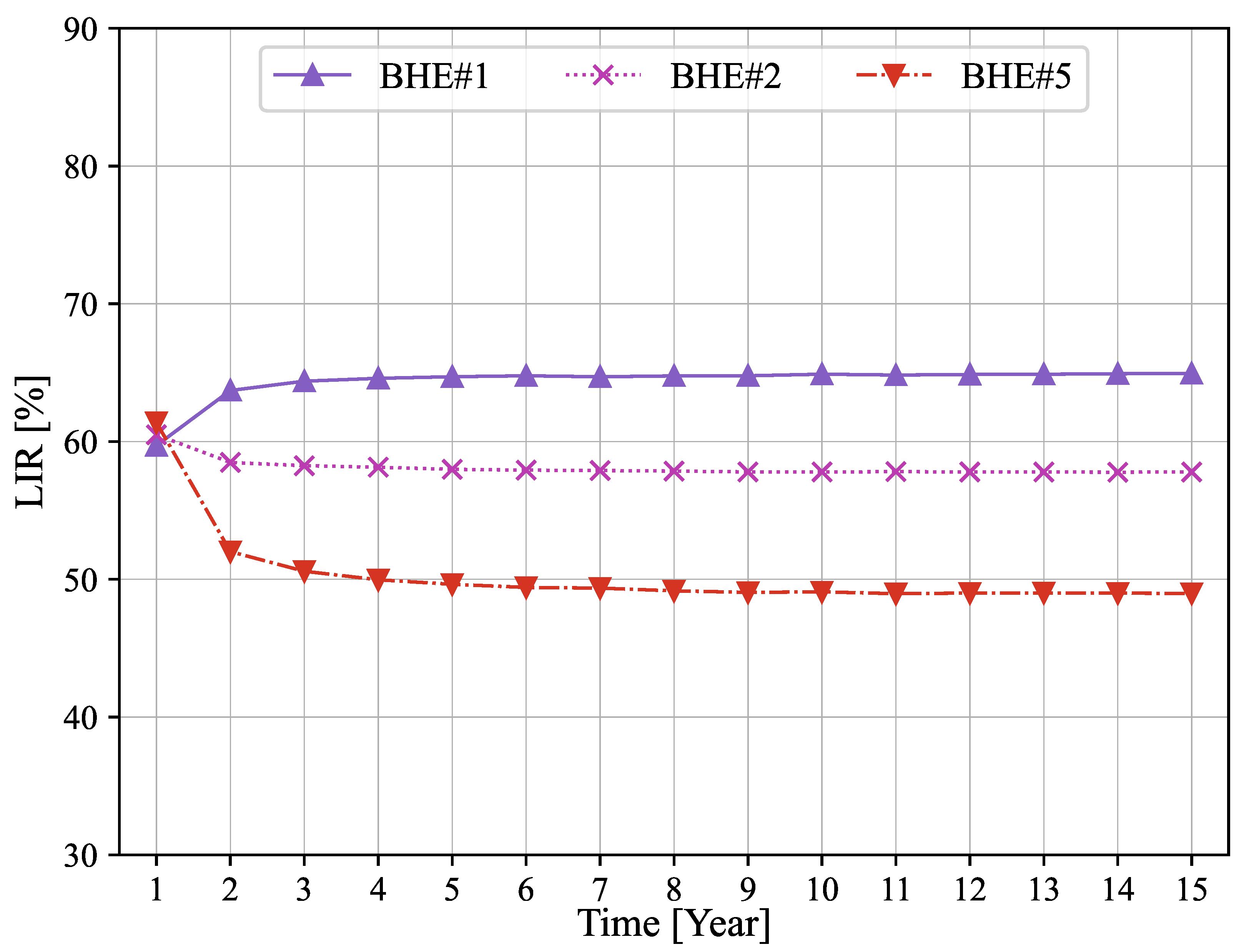
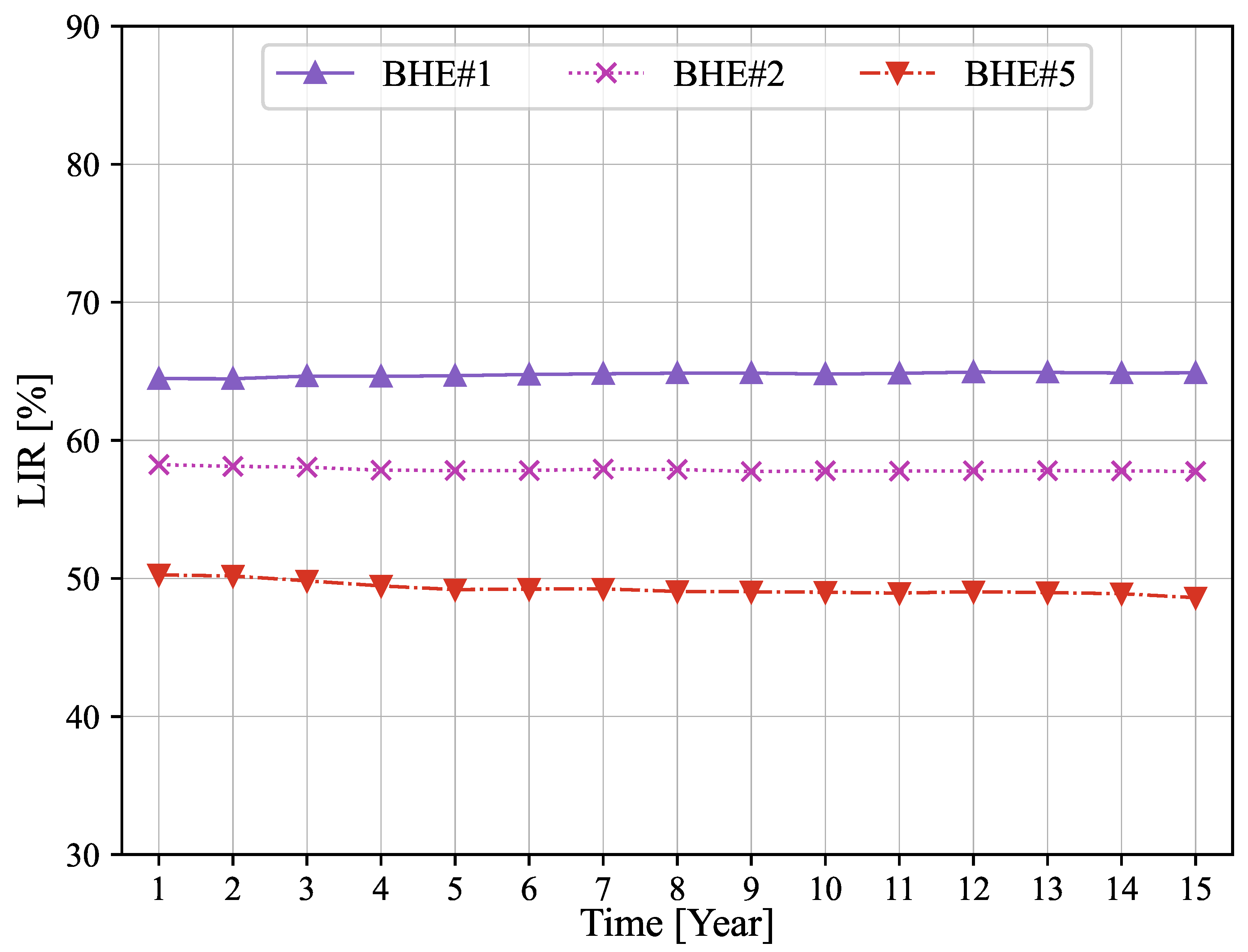
4.2.2. Influence of Borehole Location on LIR

When the cooling capacity and heating capacity imposed on the MSBHE array are determined, the load imbalance ratio for the whole MSBHE array will be set to a certain value. However, Figure 9 shows that the outlet temperature of MSBHE #1, #2, and #5 is not the same. The cooling and heating capacity for each MSBHEs in the array are not equal, which means the load imbalance ratios for each MSBHE are different. This load-shifted phenomenon has been reported by the work of Chen et al. [53]. Δ Q refers to the shifted load of selected MSBHEs, determined by subtracting the system’s average cooling and heating capacity from the cooling and heating capacity of each MSBHE. When Δ Q is positive, the selected MSBHE provides more cold in the cooling season and less heat in the heating season. On the contrary, the MSBHE provides less cold in the cooling season and more heat in the heating season. Then, the shifted load is further normalized by the average value to show its proportion (denoted by P). When P is positive, the MSBHE provides more cold and heat. On the contrary, the MSBHE provides less cold and heat.
Figure 11 shows that it takes four years for the MSBHE system to reach the quasi-steady state in the cooling season and three years in the heating season. MSBHE #5 provided less cold than the system average in the first cooling season, while MSBHE #1 and #2 were higher than the system average. From the second year, MSBHE #5 provided more cooling capacity at the beginning of the cooling season and less capacity at the end. The trend of MSBHE #1 and #2 is opposite to #5. It shows that heat accumulation occurs at the end of the cooling season. Before reaching the quasi-steady state, the shifted load of MSBHE #5 is negative at the beginning of the heating season, which means the heat extracted by MSBHE #5 is higher than the system average. Then, this shifted load value becomes positive, which means the heat provided is lower than the system average. Meanwhile, the variation trend for the shifted load of MSBHE #1 and #2 in the first three years is just opposite to MSBHE #5. From the fourth heating season, the shifted load of MSBHE #2 and #5 is always positive, which means that the heat provided by the MSBHEs is lower than the average value, and this part will be supplied by MSBHE #1. This phenomenon shows that cold accumulation will occur in the heating season. Compared with the other two MSBHEs, the shifted load of MSBHE #5 is always the largest, which means that the accumulation of cooling and heating load in the soil has the most significant impact on the performance of the MSBHE located in the middle. The shifted load of the MSBHEs decreases in the cooling season while increasing in the heating season, indicating that the heat dissipation effect of soil in the cooling season and the heat supplement effect in the heating season are gradually ineffective. On the other hand, the shifted load variation can be deduced according to the proportion compared with the average value.
As can be seen from Figure 11, after the system reaches a quasi-steady state, the positive and negative signs of the proportion P of the same MSBHE are opposite in the cooling and heating season. This means that the shifted load trend of the MSBHE system is the opposite in the cooling and heating season. When the heat exchanger provides more cold in the cooling season, it will provide less heat in the heating season, such as MSBHE #2 and #5. When it provides less cold in the cooling season, it will provide more heat in the heating season, such as MSBHE #1. Moreover, the maximum P value reaches 33.42% in the cooling season and 19.96% in the heating season, which indicates that the shifted load phenomenon of the MSBHE array system is more severe in the cooling season.
The load imbalance ratio for each MSBHE can be calculated according to Equation (1). As shown in Figure 12, the load imbalance ratio of MSBHE #1 increased from 59.71% in the first year to 64.95% in the 15th year. On the contrary, the load imbalance ratio of MSBHE #2 and MSBHE #5 is gradually decreasing, the load imbalance ratio of MSBHE #2 is reduced from 60.49% to 57.79%, and the load imbalance ratio of MSBHE #5 is reduced from 61.39% to 48.97%. The load imbalance ratio of the three MSBHEs changed considerably in the first two years, then remained unchanged in the following years. Among them, the load imbalance ratio of MSBHE #5 is the lowest because MSBHE #5 has the strongest cooling capacity and the weakest heating capacity (see Figure 11). Compared with a single MSBHE and MSBHE array, only the thermal imbalance rate of MSBHE #1 located at the edge of the group is greater than that of a single MSBHE. This illustrates that the accumulation of cooling load will reduce the load imbalance ratio of MSBHE.

5. Discussion

5.1. Extended Numerical Simulation

In scenario #6, the MSBHE system starts operation from the cooling season. When the system started an operation in the first year, the bottom soil temperature surrounding the MSBHEs was too high, resulting in the change of the shifted load of the MSBHEs in the previous years after reaching the quasi-steady state. Therefore, a new scenario #7, which runs from the heating season, is set, and the other parameters are the same as scenario #6. Figure 13 shows the evolution of the load imbalance ratio of MSBHEs under scenario #7. It can be seen that the load imbalance ratio of the three MSBHEs is barely unchanged, and the value is equal to that after the system reaches a quasi-steady state in scenario #6. It shows that when the system starts to operate from the heating season, the MSBHEs absorb heat from the soil and the soil temperature will decrease. Therefore, the soil temperature will not be higher than the circulating fluid temperature during the cooling season. This helps the MSBHE system to provide cooling for the buildings. Therefore, the MSBHE system is suggested to start running from the heating season in the actual application process.

5.2. Future Work

The existing studies on the load imbalance ratio are often based on short-term simulations [16], and the depth of the borehole heat exchanger is basically within 200 m [16,17]. In this work, we proposed a new type of medium-shallow borehole heat exchanger, which breaks through the 200-meter limit of conventional shallow BHE. Through comprehensive numerical modeling over a long-term period, the sustainable load imbalance ratios of the MSBHE system under several design parameters are carefully quantified. It is worth noting that other system parameters, including soil physical parameters, drilling spacing, and pipe network arrangement, will also have considerable influence on the load imbalance ratio of the MSBHE array system. In addition, the initial investment of the MSBHE system will be higher than the conventional BHE system because of the deeper drilling depth; thus, it is crucial to analyze the economic feasibility in the practical project application. The medium-shallow borehole heat exchanger system introduced in this article has been implemented in a practical project in Xi’an, China. It is expected to be put into actual use in 2023. Based on the in situ measurement data, further investigation of the MSBHE system and corresponding optimization method will be discussed in our future research.

6. Conclusions

In this paper, a new type of medium-shallow borehole heat exchanger (MSBHE) system is proposed and established based on the geological parameters of Xi’an. Then, the MSBHE system is simulated by OGS-TESPy software, which reveals the long-term performance and sustainability of MSBHE in the area with unbalanced cooling and heating load of buildings. The main findings of this paper are as follows.
By increasing the borehole depth, the sustainable load imbalance ratio of MSBHE will increase. According to the simulation results, when the drilling depth increases from 200 m to 500 m, the load imbalance ratio increases from 20.76% to 60.29%. When the drilling depth is the same, the influence of the circulating fluid inlet velocity and the operation mode of the system on the load imbalance ratio can be neglected.
The load imbalance ratio of heat exchangers in different locations of the MSBHE array is different. The MSBHE located in the middle of the array has the lowest load imbalance ratio of 48.97%, which is 15.98% lower than the borehole in the edge location. In addition, the trend of shifted load variation in the system during the cooling season is opposite to the heating season. The heat exchanger, which provides more cooling load, will provide less heating load and vice versa. Finally, the extended numerical simulation results show that the system starting from the heating season is recommended due to the quick achievement of a quasi-steady state.
The newly proposed MSBHE in this work can sustain a notable load imbalance ratio, which is particularly applicable to the areas with a strong imbalance of annual building load. Furthermore, the research in this paper provides new knowledge for the geothermal research community and gives suggestions for the design of the MSBHE system.

Author Contributions

R.W.: Conceptualization, methodology, software, validation, writing—original draft, visualization. F.W.: Conceptualization, project administration, funding acquisition, supervision. Y.X.: investigation, data curation. J.J.: investigation, formal analysis, visualization. Y.Z.: project administration, resources. W.C.: Conceptualization, methodology, software, writing—review and editing, supervision. C.C.: methodology, software, validation, writing—review and editing. All authors have read and agreed to the published version of the manuscript.

Funding

This research was funded by the Key Research and Development Project of Shaanxi Province (2020ZDLSF06-08) and the Open Project of Key Laboratory of Coal Resources Exploration and Comprehensive Utilization (ZP2020-1, KF2021-1).

Institutional Review Board Statement

Not applicable.

Informed Consent Statement

Not applicable.

Data Availability Statement

The data presented in this study are available on request for the interested readers.

Conflicts of Interest

The authors declare no conflict of interest.

Abbreviations

The following abbreviations are used in this manuscript:
GSHPGround Source Heat Pump
BHEBorehole Heat Exchange
DBHEDeep Borehole Heat Exchange
FLSfinite line source
MSBHEmedium-shallow borehole heat exchange
1Usingle-U
2Udouble-U
CXCcoaxial with centered inlet
CXAcoaxial with annular inlet
OGSOpenGeoSys
DC-FEMdual-continuum finite element metho
TESPyThermal Engineering System in Python
LIRload imbalance ratio (%)
Q A H I accumulated heat imposed on the MSBHE (J)
Q A C S accumulated cooling supplied by the MSBHE (J)
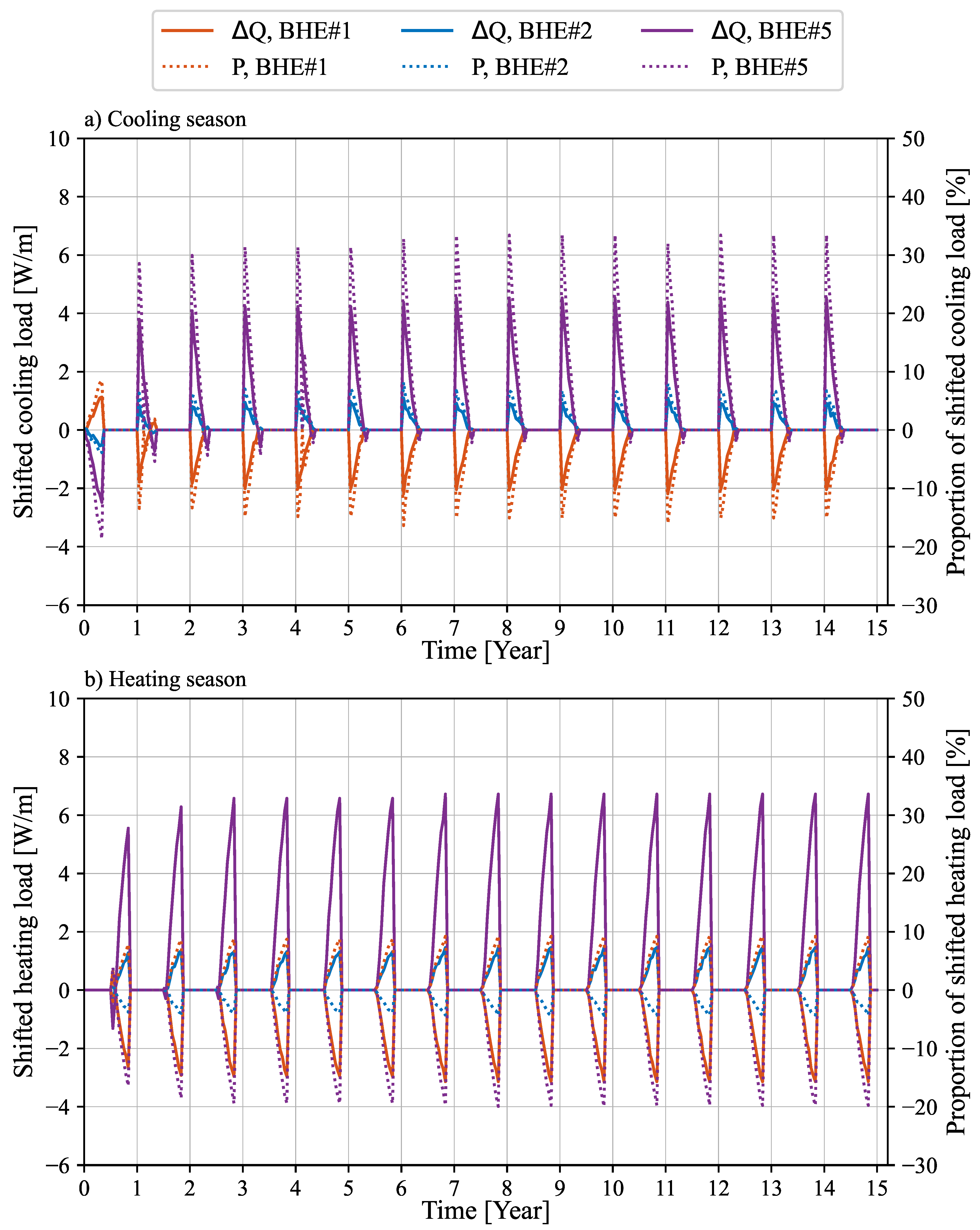
Δ Qshifted load (W/m)
Pproportion of shifted load (%)

References

  1. Pramit, V.; Tanu, K.; Akhilesh, S.R. Energy emissions, consumption and impact of urban households: A review. Renew. Sustain. Energy Rev. 2021, 147, 111210. [Google Scholar] [CrossRef]
  2. Melike, E.B.; Seyit, M. Gökmenoğlu. Environmental pollution, hydropower energy consumption and economic growth: Evidence from G7 countries. Renew. Sustain. Energy Rev. 2017, 75, 68–85. [Google Scholar] [CrossRef]
  3. Jia, Z.J.; Lin, B.Q. How to achieve the first step of the carbon-neutrality 2060 target in China: The coal substitution perspective. Energy 2021, 233, 121179. [Google Scholar] [CrossRef]
  4. Arnulf, J.W.; Ioannis, K.; Nigel, T.; Christian, T. How photovoltaics can contribute to GHG emission reductions of 55% in the EU by 2030. Renew. Sustain. Energy Rev. 2020, 126, 109836. [Google Scholar] [CrossRef]
  5. Zhang, S.C.; Fu, Y.J.; Yang, X.Y.; Xu, W. Assessment of mid-to-long term energy saving impacts of nearly zero energy building incentive policies in cold region of China. Energy Build. 2021, 241, 110938. [Google Scholar] [CrossRef]
  6. Austin, A.; Behnaz, R. Geothermal technology: Trends and potential role in a sustainable future. Appl. Energy 2019, 248, 18–34. [Google Scholar] [CrossRef]
  7. Soltani, M.; Kashkooli, F.M.; Souri, M.; Rafiei, B.; Jabarifar, M.; Gharali, K.; Nathwani, J.S. Environmental, economic, and social impacts of geothermal energy systems. Renew. Sustain. Energy Rev. 2021, 140, 110750. [Google Scholar] [CrossRef]
  8. John, W.L.; Aniko, N.T. Direct utilization of geothermal energy 2020 worldwide review. Geothermics 2021, 90, 101915. [Google Scholar] [CrossRef]
  9. Zhao, X.G.; Wan, G. Current situation and prospect of China’s geothermal resources. Renew. Sustain. Energy Rev. 2014, 32, 651–661. [Google Scholar] [CrossRef]
  10. Xu, Y.S.; Wang, X.W.; Shen, S.L.; Zhou, A.N. Distribution characteristics and utilization of shallow geothermal energy in China. Energy Build. 2020, 229, 110479. [Google Scholar] [CrossRef]
  11. China Geological Survey, Ministry of Natural Resources; Department of New and Renewable Energy, National Energy. China Geothermal Energy Development Report; China Petrochemical Press: Beijing, China, 2018.
  12. Wang, F.H.; Cai, W.L.; Wang, M.; Gao, Y.; Liu, J.; Wang, Z.H.; Xu, H. Status and Outlook for Research on Geothermal Heating Technology. J. Refrig. 2021, 42, 14–22. [Google Scholar] [CrossRef]
  13. Cai, W.L.; Wang, F.H.; Chen, S.; Chen, C.F.; Liu, J.; Deng, J.W.; Olaf, K.; Shao, H.B. Analysis of heat extraction performance and long-term sustainability for multiple deep borehole heat exchanger array: A project-based study. Appl. Energy 2021, 289, 116590. [Google Scholar] [CrossRef]
  14. Li, J.; Xu, W.; Li, J.F.; Huang, S.; Li, Z.; Qiao, B.; Yang, C.; Sun, D.Y.; Zhang, G.Q. Heat extraction model and characteristics of coaxial deep borehole heat exchanger. Renew. Energy 2021, 169, 738–751. [Google Scholar] [CrossRef]
  15. Demba, N. Reliability and performance of direct-expansion ground-coupled heat pump systems: Issues and possible solutions. Renew. Sustain. Energy Rev. 2016, 66, 802–814. [Google Scholar] [CrossRef]
  16. Yang, W.B.; Chen, Y.P.; Shi, M.H.; Jeffrey, D.S. Numerical investigation on the underground thermal imbalance of ground-coupled heat pump operated in cooling-dominated district. Appl. Therm. Eng. 2013, 58, 626–637. [Google Scholar] [CrossRef]
  17. Qian, H.; Wang, Y.G. Modeling the interactions between the performance of ground source heat pumps and soil temperature variations. Energy Sustain. Dev. 2014, 23, 115–121. [Google Scholar] [CrossRef]
  18. Hou, G.Y.; Hessam, T.; Song, Y.; Jiang, W.; Chen, D.Y. A systematic review on optimal analysis of horizontal heat exchangers in ground source heat pump systems. Renew. Sustain. Energy Rev. 2022, 154, 111830. [Google Scholar] [CrossRef]
  19. Denis, G.; Ruchi, C.; Kenichi, S. Risk based lifetime costs assessment of a ground source heat pump (GSHP) system design: Methodology and case study. Build. Environ. 2013, 60, 66–80. [Google Scholar] [CrossRef]
  20. Ladislaus, R.; Walter, J.E. Sustainability aspects of geothermal heat pump operation, with experience from Switzerland. Geothermics 2010, 39, 365–369. [Google Scholar] [CrossRef]
  21. Ruiz-Calvo, F.; Cervera-Vázquez, J.; Montagud, C.; Corberán, J.M. Reference data sets for validating and analyzing GSHP systems based on an eleven-year operation period. Geothermics 2016, 64, 538–550. [Google Scholar] [CrossRef]
  22. Ruiz-Calvo, F.; Montagud, C. Reference data sets for validating GSHP system models and analyzing performance parameters based on a five-year operation period. Geothermics 2014, 51, 417–428. [Google Scholar] [CrossRef]
  23. Pan, S.; Kong, Y.; Chen, C.; Pang, Z.; Wang, J. Optimization of the utilization of deep borehole heat exchangers. Geotherm. Energy 2020, 8, 1–20. [Google Scholar] [CrossRef]
  24. Selvaraj, S.N.; Simon, J.R. Performance analysis of a large geothermal heating and cooling system. Renew. Energy 2018, 122, 429–442. [Google Scholar] [CrossRef] [Green Version]
  25. Adam, M.; Dante, F.; James, M.T.; David, J.H. Long-term district-scale geothermal exchange borefield monitoring with fiber optic distributed temperature sensing. Geothermics 2018, 72, 193–204. [Google Scholar] [CrossRef]
  26. Li, M.; Alvin, C.K.L. Review of analytical models for heat transfer by vertical ground heat exchangers (GHEs): A perspective of time and space scales. Appl. Energy 2015, 151, 178–191. [Google Scholar] [CrossRef]
  27. Yang, H.; Cui, P.; Fang, Z. Vertical-borehole ground-coupled heat pumps: A review of models and systems. Appl. Energy 2010, 87, 16–27. [Google Scholar] [CrossRef]
  28. Zhang, L.F.; Zhang, Q.; Huang, G.S. A transient quasi-3D entire time scale line source model for the fluid and ground temperature prediction of vertical ground heat exchangers (GHEs). Appl. Energy 2016, 170, 65–75. [Google Scholar] [CrossRef]
  29. Luo, Y.Q.; Yu, J.H.; Yan, T.; Zhang, L.; Liu, X.B. Improved analytical modeling and system performance evaluation of deep coaxial borehole heat exchanger with segmented finite cylinder-source method. Energy Build. 2020, 212, 109829. [Google Scholar] [CrossRef]
  30. Guo, Y.; Hu, X.; Banks, J.; Liu, W.V. Considering buried depth in the moving finite line source model for vertical borehole heat exchangers—A new solution. Energy Build. 2020, 214, 109859. [Google Scholar] [CrossRef]
  31. Louis, L.; Benoit, B. A new contribution to the finite line-source model for geothermal boreholes. Energy Build. 2007, 39, 188–198. [Google Scholar] [CrossRef]
  32. Mikael, P.; Michel, B.; Dominique, M. Validity ranges of three analytical solutions to heat transfer in the vicinity of single boreholes. Geothermics 2009, 38, 407–413. [Google Scholar] [CrossRef]
  33. Li, M.; Alvin, C.K.L. Analytical model for short-time responses of ground heat exchangers with U-shaped tubes: Model development and validation. Appl. Energy 2013, 104, 510–516. [Google Scholar] [CrossRef]
  34. Alberto, C.; Michela, C.; Nicola, M.; Alessandro, M. Models for thermo-fluid dynamic phenomena in low enthalpy geothermal energy systems: A review. Renew. Sustain. Energy Rev. 2016, 60, 330–355. [Google Scholar] [CrossRef]
  35. Perego, R.; Guandalini, R.; Fumagalli, L.; Aghib, F.S.; Biase, D.L.; Bonomi, T. Sustainability evaluation of a medium scale GSHP system in a layered alluvial setting using 3D modeling suite. Geothermics 2016, 59, 14–26. [Google Scholar] [CrossRef]
  36. Lee, C.K. Effects of multiple ground layers on thermal response test analysis and ground-source heat pump simulation. Renew. Sustain. Energy Rev. 2011, 88, 4405–4410. [Google Scholar] [CrossRef]
  37. Florides, G.A.; Paul, C.; Panayiotis, P. Single and double U-tube ground heat exchangers in multiple-layer substrates. Appl. Energy 2013, 102, 364–373. [Google Scholar] [CrossRef]
  38. Nam, Y.J.; Ryozo, O.; Suckho, H. Development of a numerical model to predict heat exchange rates for a ground-source heat pump system. Energy Build. 2008, 40, 2133–2140. [Google Scholar] [CrossRef]
  39. Luo, J.; Joachim, R.; Manfred, B.; Anna, P.; Xiang, W. Analysis on performance of borehole heat exchanger in a layered subsurface. Appl. Energy 2014, 123, 55–65. [Google Scholar] [CrossRef]
  40. Hu, X.C.; Jonathan, B.; Wu, L.P.; Liu, W.V. Numerical modeling of a coaxial borehole heat exchanger to exploit geothermal energy from abandoned petroleum wells in Hinton, Alberta. Renew. Energy 2020, 148, 1110–1123. [Google Scholar] [CrossRef]
  41. Li, C.; Guan, Y.L.; Liu, J.H.; Jiang, C.; Yang, R.T.; Hou, X.M. Heat transfer performance of a deep ground heat exchanger for building heating in long-term service. Renew. Energy 2020, 166, 20–34. [Google Scholar] [CrossRef]
  42. Luo, J.; Joachim, R.; Manfred, B.; Anna, P.; Lucas, W.; Xiang, W. Heating and cooling performance analysis of a ground source heat pump system in Southern Germany. Geothermics 2015, 53, 57–66. [Google Scholar] [CrossRef]
  43. Zhai, X.Q.; Cheng, X.W.; Wang, R.Z. Heating and cooling performance of a minitype ground source heat pump system. Appl. Therm. Eng. 2017, 111, 1366–1370. [Google Scholar] [CrossRef]
  44. Chen, S.; Francesco, W.; Olaf, K.; Shao, H.B. Shifted thermal extraction rates in large Borehole Heat Exchanger array—A numerical experiment. Appl. Therm. Eng. 2020, 167, 114750. [Google Scholar] [CrossRef]
  45. Bilke, L. OpenGeoSys Tutorial. Available online: https://www.opengeosys.org/docs/userguide/basics/introduction/ (accessed on 15 January 2022).
  46. Philipp, H.; Olaf, K.; Uwe-Jens, G.; Anke, B.; Shao, H.B. A numerical study on the sustainability and efficiency of borehole heat exchanger coupled ground source heat pump systems. Appl. Therm. Eng. 2016, 100, 421–433. [Google Scholar] [CrossRef]
  47. Francesco, W.; Ilja, T. TESPy: Thermal Engineering Systems in Python. J. Open Source Softw. 2020, 5, 2178. [Google Scholar]
  48. Bell, I.H.; Wronski, J.; Quoilin, S.; Lemort, V. Pure and Pseudo-pure Fluid Thermophysical Property Evaluation and the Open-Source Thermophysical Property Library CoolProp. Ind. Eng. Chem. Res. 2014, 53, 2498–2508. [Google Scholar] [CrossRef] [Green Version]
  49. Moldovan, D.; Peeters, F. Pybinding v0.8.0: A Python package for tight-binding calculations. Zenodo 2016. [Google Scholar] [CrossRef]
  50. Witte, F. TESPy Documentation. Available online: https://tespy.readthedocs.io/en/master/ (accessed on 20 January 2022).
  51. National Meteorological Information Center. Data Set of Monthly Standard Values of Surface Climate in CHINA (1981–2010). Available online: http://data.cma.cn/ (accessed on 10 February 2022).
  52. Zhou, Y.; Mu, G.X.; Zhang, H.; Wang, K.; Liu, J.Q.; Zhang, Y.G. Geothermal field division and its geological influencing factors in Guanzhong basin. Geol. China 2017, 44, 1017–1026. [Google Scholar] [CrossRef]
  53. Chen, S.; Cai, W.L.; Francesco, W.; Wang, X.R.; Wang, F.H.; Olaf, K.; Shao, H.B. Long-term thermal imbalance in large borehole heat exchangers array—A numerical study based on the Leicester project. Energy Build. 2021, 231, 110518. [Google Scholar] [CrossRef]
  54. Jakob, R.; Chen, S.; Katrin, L.; Steve, T.; Tom, R.; Karsten, R.; Rüdiger, G.; Anke, B.; Olaf, K.; Shao, H.B. Modeling Neighborhood-Scale Shallow Geothermal Energy Utilization-A Case Study in Berlin. Geotherm. Energy 2022, 10, 1–26. [Google Scholar] [CrossRef]
  55. Richard, A.B. Thermal response tests on deep borehole heat exchangers with geothermal gradient. Appl. Therm. Eng. 2020, 178, 115447. [Google Scholar] [CrossRef]
  56. GB50366; Technical Code for Ground-Source Heat Pump System. Ministry of Housing and Urban-Rural Development: Beijing, China, 2009.
Figure 1. The outlet temperature and simulation time of OGS under different grid densities and time steps.
Energies 15 03444 g001
Figure 2. Verification of proposed MSBHE model based on OpenGeoSys against Beier’s analytical solution.
Energies 15 03444 g002
Figure 3. Comparison of the outlet temperature of MSBHE under three scenarios.
Energies 15 03444 g003
Figure 4. Maximum cooling and heating load of MSBHE and LIR under different depths.
Energies 15 03444 g004
Figure 5. Maximum cooling and heating load of MSBHE and LIR under different flow rates.
Energies 15 03444 g005
Figure 6. Maximum cooling and heating load of MSBHE and LIR under different model operations.
Energies 15 03444 g006
Figure 7. Location of the MSBHEs in the subsurface model.
Energies 15 03444 g007
Figure 8. Evolution of inflow and outflow temperature of BHE #5 in the end of (a) cooling season and (b) heating season over 15 years.
Energies 15 03444 g008
Figure 9. Evolution of inflow and outflow temperature of the selected MSBHEs in the end of (a) cooling season and (b) heating season under scenario #6 over 15 years.
Energies 15 03444 g009
Figure 10. Evolution of soil temperature over 15 years at 1 m distance from the selected MSBHEs at a depth of 505 m in the end of cooling, heating, and recovery season.
Energies 15 03444 g010
Figure 11. Evolution and the proportion of the shifted load in the (a) cooling season and (b) heating season over 15 years.
Energies 15 03444 g011
Figure 12. Evolution of the load imbalance ratio of the selected MSBHE over 15 years.
Energies 15 03444 g012
Figure 13. Evolution of the load imbalance ratio of the selected MSBHE under scenario #7 over 15 years.
Energies 15 03444 g013
Table 1. Detailed parameters of the coaxial MSBHE system.
ItemParameterUnitValue
Boreholedepth500m
diameter0.15m
Outer diameter of outer pipe0.1143m
Outer diameter of inner tube0.042m
Wall thickness of outer pipe0.00688m
Wall thickness of inner tube wall0.01m
Thermal conductivity of outer pipe wall14.48W m 1 K 1
Thermal conductivity of inner tube wall0.02W m 1 K 1
GroutDensity2190Kg m 3
Specific heat capacity1735.16J Kg 1 K 1
Thermal conductivity0.73W m 1 K 1
Circulating fluidDensity998Kg m 3
Specific heat capacity4190J Kg 1 K 1
Thermal conductivity0.6W m 1 K 1
Dynamic viscosity9.31 × 10 4 Kg m 1 s 1
SubsurfaceGeothermal gradient31.5 ° C km 1
Soil density1120Kg m 3
Soil specific heat capacity1780J Kg 1 K 1
Soil thermal conductivity2.4W m 1 K 1
Table 2. Different scenarios of the MSBHE system.
ItemLoad in Cooling SeasonLoad in Heating Season
Per Meter (W m 1 )Total (kW)Per Meter (W m 1 )Total (kW)
scenario 12713.56834
scenario 22713.56934.5 (+0.5)
scenario 32814 (+0.5)6834
Publisher’s Note: MDPI stays neutral with regard to jurisdictional claims in published maps and institutional affiliations.

