
Machine Learning Short-Term Energy Consumption Forecasting for Microgrids in a Manufacturing Plant


Abstract
:1. Introduction
2. Forecasting Methods for Smart Grids
3. Proposed Methodology
3.1. Proposed Machine Learning Model and Data Characteristics
- (1)
- Energy use data—the time range for which forecasting is made;
- (2)
- Application for the end-user—the model needs to forecast energy consumption without the employment of expensive software, and therefore, the proposed solution is a utility that is easy to use and does not require knowledge in forecasting techniques;
- (3)
- The character of the measurement data—the shape of the input vector and the number of data points impact the preparation of training and test datasets;
- (4)
- Automation of energy prediction forecasting.
3.1.1. Dataset Exploited in this Study
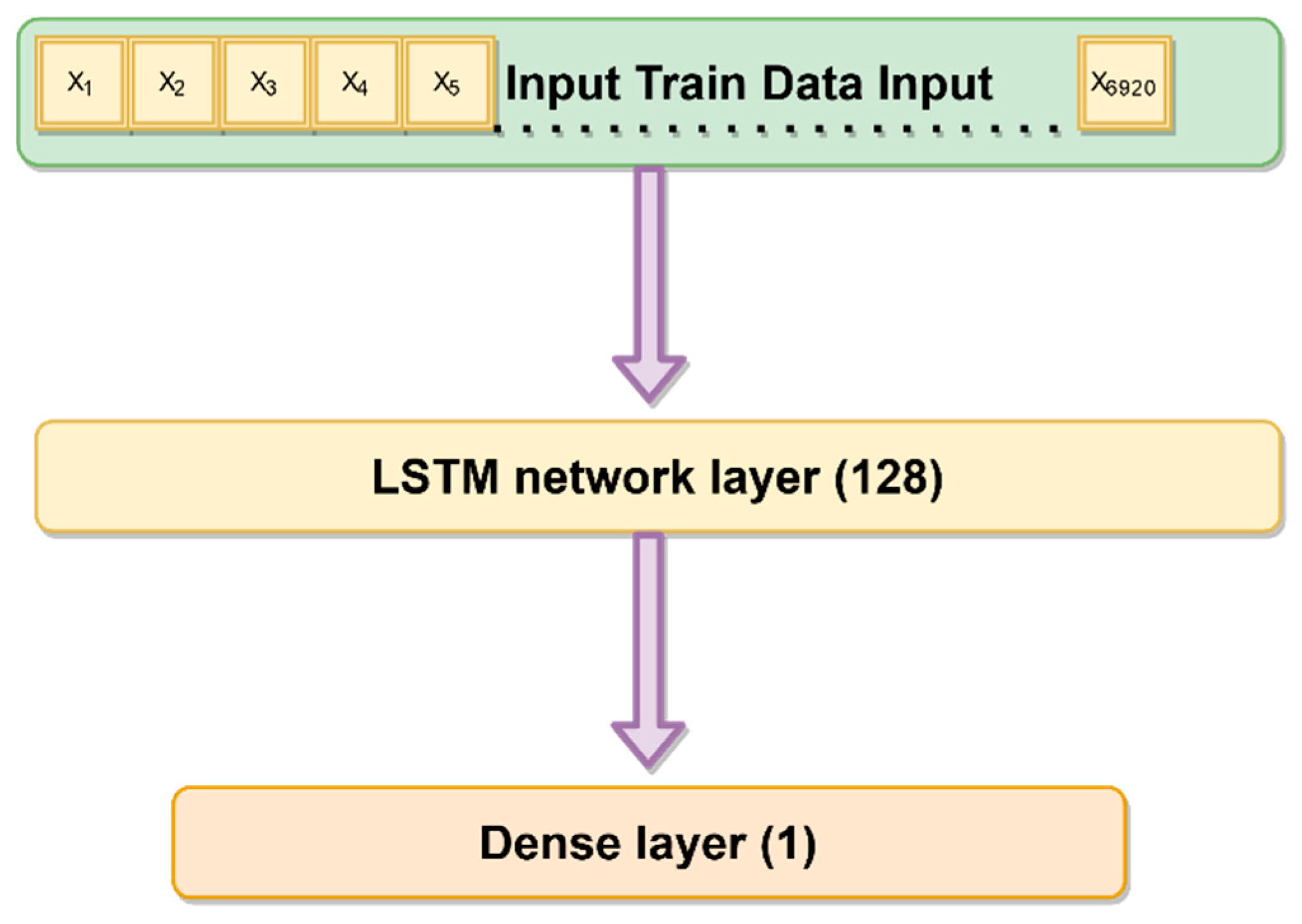
3.1.2. Machine Learning Model
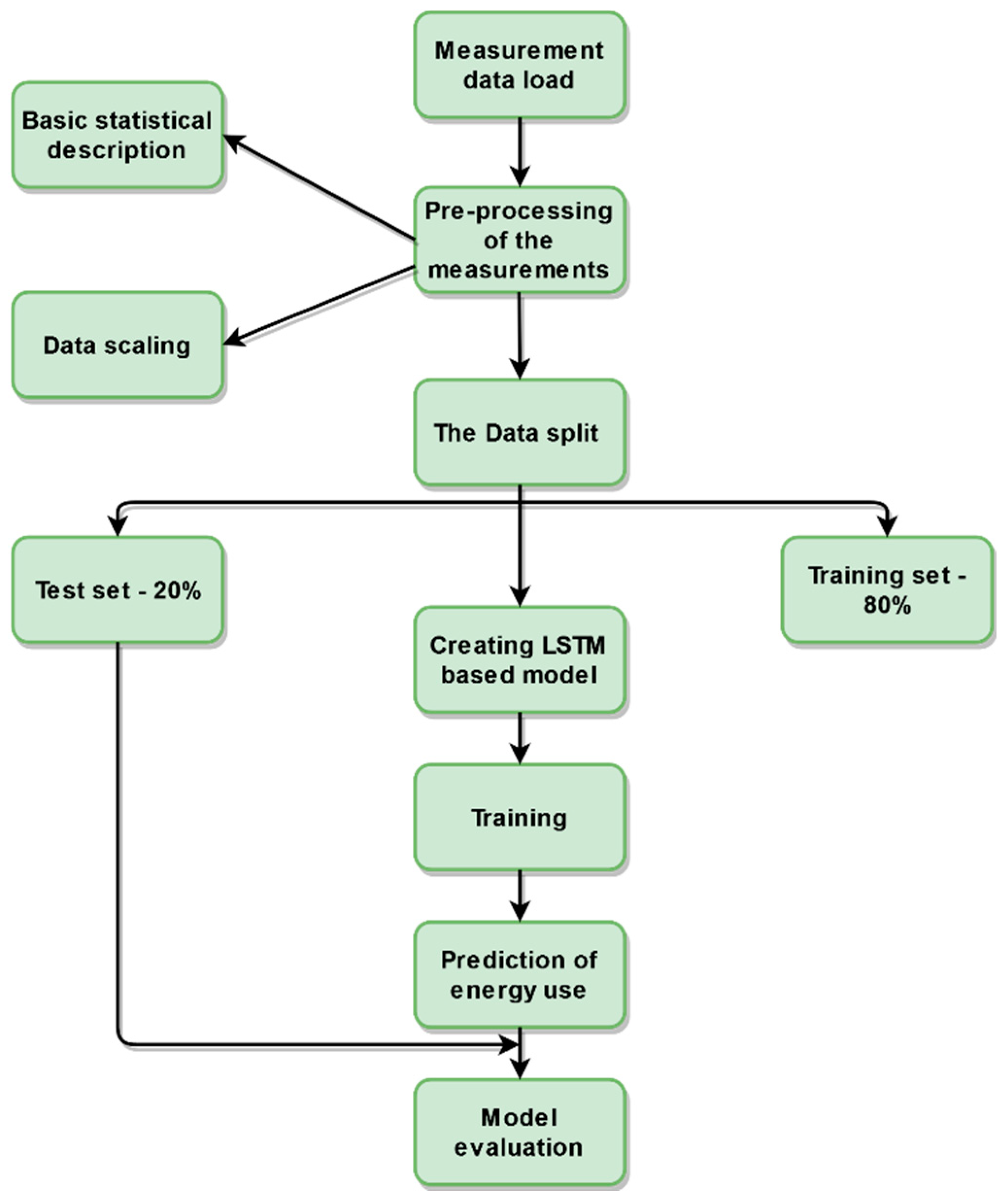
3.2. Deep Learning Process
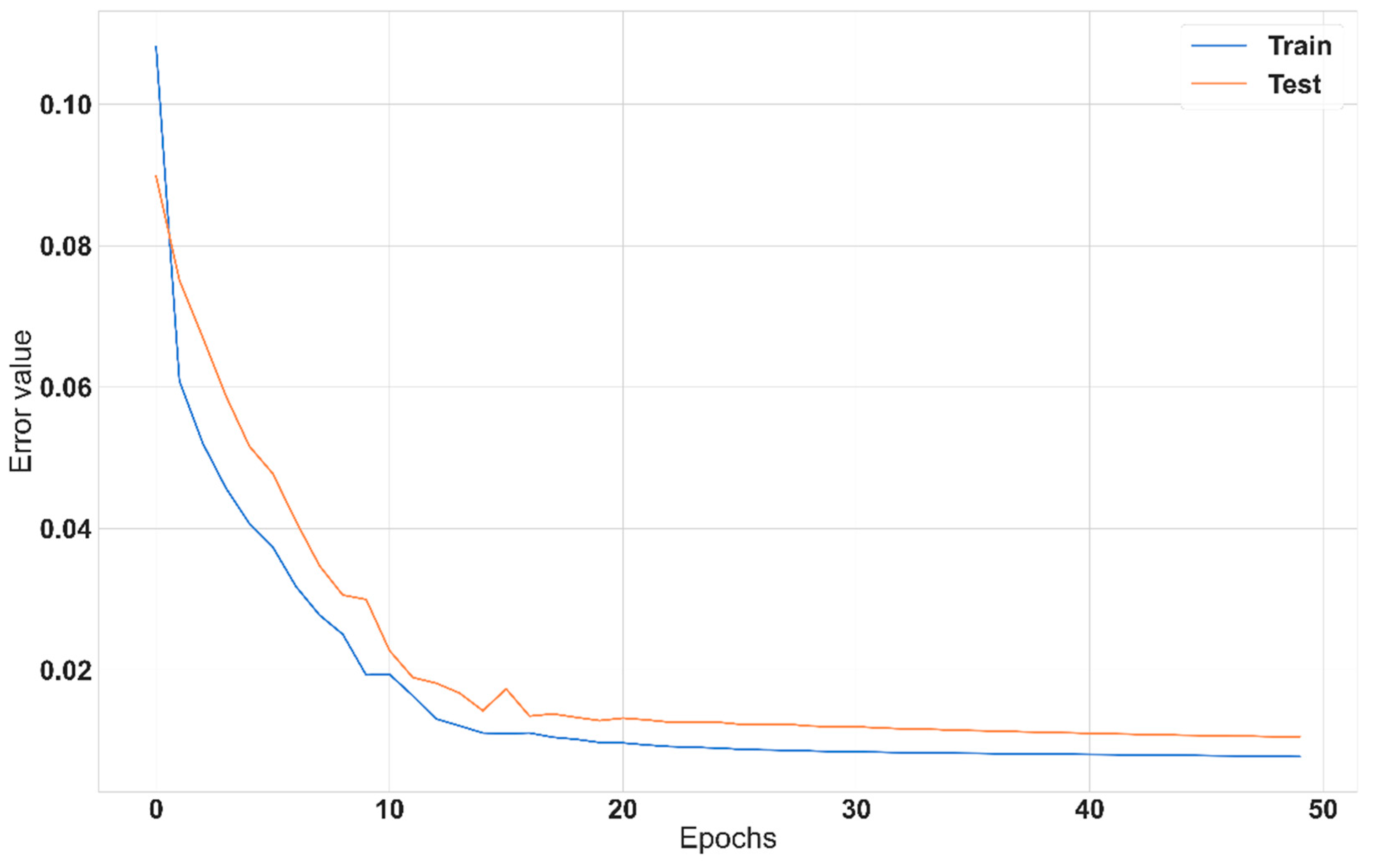
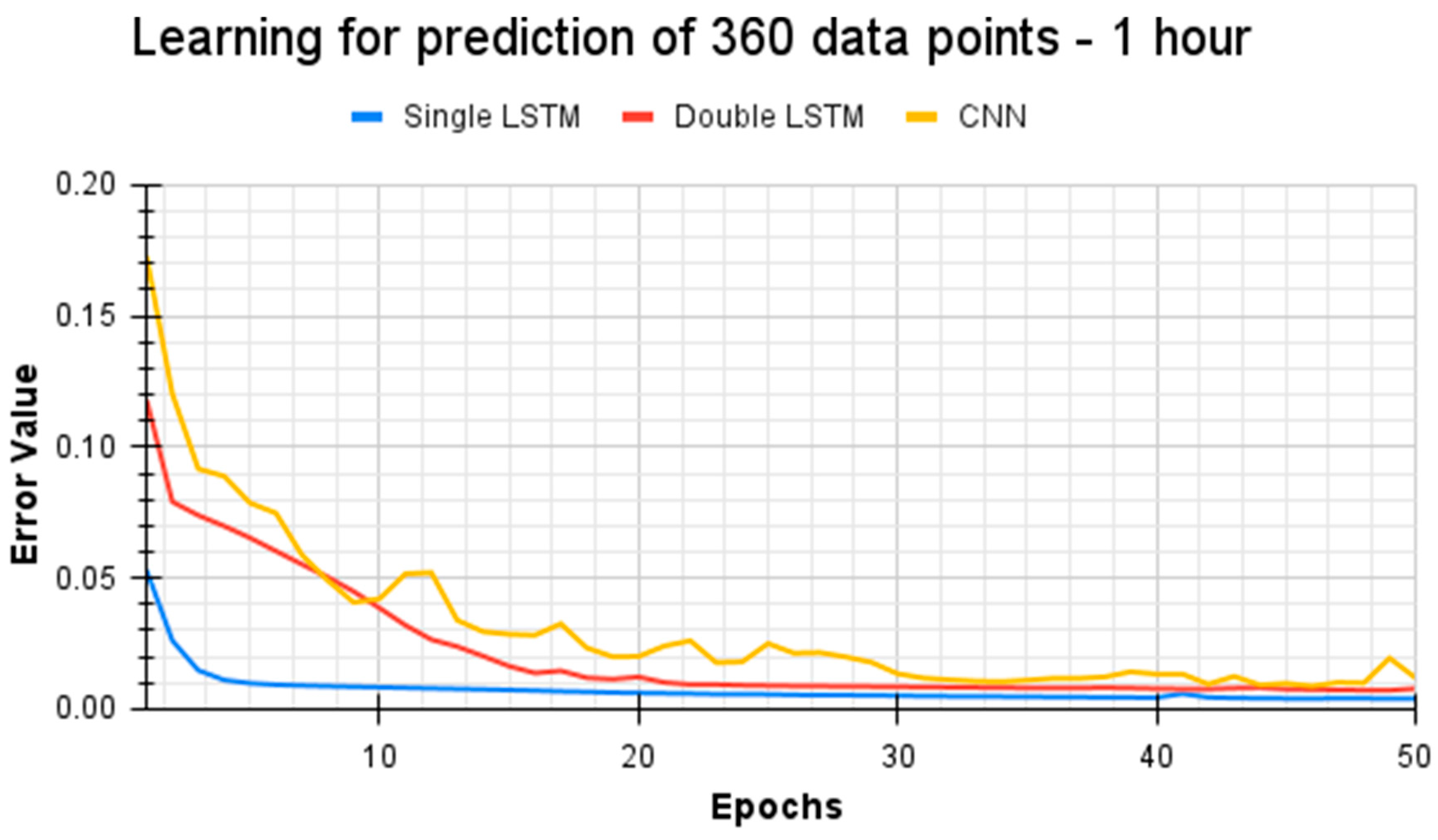
4. Results
5. Discussion
6. Conclusions
Author Contributions
Funding
Data Availability Statement
Conflicts of Interest
References
- Considine, T.; Cox, W.; Cazalet, E.G. Understanding Microgrids as the Essential Architecture of Smart Energy. In Proceedings of the Grid-Interop Forum 2012, Irving, TX, USA, 3–6 December 2012. [Google Scholar] [CrossRef]
- Ma, J.; Ma, X. A Review of Forecasting Algorithms and Energy Management Strategies for Microgrids. Syst. Sci. Control. Eng. 2018, 6, 237–248. [Google Scholar] [CrossRef]
- Worighi, I.; Maach, A.; Hafid, A.; Hegazy, O.; Van Mierlo, J. Integrating Renewable Energy in Smart Grid System: Architecture, Virtualization and Analysis. Sustain. Energy Grids Netw. 2019, 18, 100226. [Google Scholar] [CrossRef]
- Sabzehgar, R.; Amirhosseini, D.Z.; Rasouli, M. Solar Power Forecast for a Residential Smart Microgrid Based on Numerical Weather Predictions Using Artificial Intelligence Methods. J. Build. Eng. 2020, 32, 101629. [Google Scholar] [CrossRef]
- Alotaibi, I.; Abido, M.A.; Khalid, M.; Savkin, A.V. A Comprehensive Review of Recent Advances in Smart Grids: A Sustainable Future with Renewable Energy Resources. Energies 2020, 13, 6269. [Google Scholar] [CrossRef]
- Shulyma, O.; Shendryk, V.; Baranova, I.; Marchenko, A. The Features of the Smart MicroGrid as the Object of Information Modeling. In Information and Software Technologies, 2nd ed.; Dregvaite, G., Damasevicius, R., Eds.; Communications in Computer and Information Science; Springer International Publishing: Cham, Switzerland, 2014; Volume 465, pp. 12–23. [Google Scholar] [CrossRef]
- Palma-Behnke, R.; Reyes, L.; Jimenez-Estevez, G. Smart Grid Solutions for Rural Areas. In Proceedings of the 2012 IEEE Power and Energy Society General Meeting, San Diego, CA, USA, 22–26 July 2012; pp. 1–6. [Google Scholar] [CrossRef]
- Masembe, A. Reliability Benefit of Smart Grid Technologies: A Case for South Africa. J. Energy S. Afr. 2015, 26, 2–9. [Google Scholar] [CrossRef]
- Samad, T.; Kiliccote, S. Smart Grid Technologies and Applications for the Industrial Sector. Comput. Chem. Eng. 2012, 47, 76–84. [Google Scholar] [CrossRef]
- Keller, F.; Schultz, C.; Simon, P.; Braunreuther, S.; Glasschröder, J.; Reinhart, G. Integration and Interaction of Energy Flexible Manufacturing Systems within a Smart Grid. Procedia CIRP 2017, 61, 416–421. [Google Scholar] [CrossRef]
- Shahid, A. Smart Grid Integration of Renewable Energy Systems. In Proceedings of the 2018 7th International Conference on Renewable Energy Research and Applications (ICRERA), Paris, France, 14–17 October 2018; pp. 944–948. [Google Scholar] [CrossRef]
- Yaprakdal, F.; Yılmaz, M.B.; Baysal, M.; Anvari-Moghaddam, A. A Deep Neural Network-Assisted Approach to Enhance Short-Term Optimal Operational Scheduling of a Microgrid. Sustainability 2020, 12, 1653. [Google Scholar] [CrossRef]
- Elattar, E.E.; Sabiha, N.A.; Alsharef, M.; Metwaly, M.K.; Abd-Elhady, A.M.; Taha, I.B.M. Short Term Electric Load Forecasting Using Hybrid Algorithm for Smart Cities. Appl. Intell. 2020, 50, 3379–3399. [Google Scholar] [CrossRef]
- Wood, D.A. Hourly-Averaged Solar plus Wind Power Generation for Germany 2016: Long-Term Prediction, Short-Term Forecasting, Data Mining and Outlier Analysis. Sustain. Cities Soc. 2020, 60, 102227. [Google Scholar] [CrossRef]
- Ahmad, A.; Javaid, N.; Mateen, A.; Awais, M.; Khan, Z.A. Short-Term Load Forecasting in Smart Grids: An Intelligent Modular Approach. Energies 2019, 12, 164. [Google Scholar] [CrossRef] [Green Version]
- Wang, Y.; Huang, Y.; Wang, Y.; Li, F.; Zhang, Y.; Tian, C. Operation Optimization in a Smart Micro-Grid in the Presence of Distributed Generation and Demand Response. Sustainability 2018, 10, 847. [Google Scholar] [CrossRef] [Green Version]
- Kempener, R.; Komor, P.; Hoke, A. Smart Grids and Renewables, A Guide for Effective Deployment, Working Paper. Available online: https://www.irena.org/-/media/Files/IRENA/Agency/Publication/2013/smart_grids.pdf?la=en&hash=08F3E571B5580F017E70BCD1EC39864536681ADB (accessed on 8 October 2021).
- Siami-Namini, S.; Tavakoli, N.; Siami Namin, A. A Comparison of ARIMA and LSTM in Forecasting Time Series. In Proceedings of the 2018 17th IEEE International Conference on Machine Learning and Applications (ICMLA), Orlando, FL, USA, 17–20 December 2018; pp. 1394–1401. [Google Scholar] [CrossRef]
- Yang, H.-T.; Huang, C.-M.; Huang, C.-L. Identification of ARMAX Model for Short Term Load Forecasting: An Evolutionary Programming Approach. IEEE Trans. Power Syst. 1996, 11, 403–408. [Google Scholar] [CrossRef]
- Fang, T.; Lahdelma, R. Evaluation of a Multiple Linear Regression Model and SARIMA Model in Forecasting Heat Demand for District Heating System. Appl. Energy 2016, 179, 544–552. [Google Scholar] [CrossRef]
- Su, W.; Wang, J.; Zhang, K.; Huang, A.Q. Model Predictive Control-Based Power Dispatch for Distribution System Considering Plug-in Electric Vehicle Uncertainty. Electr. Power Syst. Res. 2014, 106, 29–35. [Google Scholar] [CrossRef]
- Emami, A.; Sarvi, M.; Asadi Bagloee, S. Using Kalman Filter Algorithm for Short-Term Traffic Flow Prediction in a Connected Vehicle Environment. J. Mod. Transport. 2019, 27, 222–232. [Google Scholar] [CrossRef] [Green Version]
- Shah, I.; Bibi, H.; Ali, S.; Wang, L.; Yue, Z. Forecasting One-Day-Ahead Electricity Prices for Italian Electricity Market Using Parametric and Nonparametric Approaches. IEEE Access 2020, 8, 123104–123113. [Google Scholar] [CrossRef]
- Aykroyd, G.R.; Alfaer, N. Sequential Models for Time-evolving Regression Problems with an Application to Energy Demand Prediction. Stoch. Modeling Appl. 2016, 20, 1–16. [Google Scholar]
- Lisi, F.; Shah, I. Forecasting Next-Day Electricity Demand and Prices Based on Functional Models. Energy Syst. 2020, 11, 947–979. [Google Scholar] [CrossRef]
- Hirose, K.; Wada, K.; Hori, M.; Taniguchi, R. Event Effects Estimation on Electricity Demand Forecasting. Energies 2020, 13, 5839. [Google Scholar] [CrossRef]
- Bibi, N.; Shah, I.; Alsubie, A.; Ali, S.; Lone, S.A. Electricity Spot Prices Forecasting Based on Ensemble Learning. IEEE Access 2021, 9, 150984–150992. [Google Scholar] [CrossRef]
- Shah, I.; Iftikhar, H.; Ali, S. Modeling and Forecasting Medium-Term Electricity Consumption Using Component Estimation Technique. Forecasting 2020, 2, 163–179. [Google Scholar] [CrossRef]
- Zhang, W.; Zhang, H.; Liu, J.; Li, K.; Yang, D.; Tian, H. Weather Prediction with Multiclass Support Vector Machines in the Fault Detection of Photovoltaic System. IEEE/CAA J. Autom. Sinica 2017, 4, 520–525. [Google Scholar] [CrossRef]
- del Real, A.J.; Dorado, F.; Durán, J. Energy Demand Forecasting Using Deep Learning: Applications for the French Grid. Energies 2020, 13, 2242. [Google Scholar] [CrossRef]
- Kang, T.; Lim, D.Y.; Tayara, H.; Chong, K.T. Forecasting of Power Demands Using Deep Learning. Appl. Sci. 2020, 10, 7241. [Google Scholar] [CrossRef]
- Kumar, S.; Hussain, L.; Banarjee, S.; Reza, M. Energy Load Forecasting Using Deep Learning Approach-LSTM and GRU in Spark Cluster. In Proceedings of the 2018 Fifth International Conference on Emerging Applications of Information Technology (EAIT), Kolkata, India, 12–13 January 2018; pp. 1–4. [Google Scholar] [CrossRef]
- Mele, E.; Elias, C.; Ktena, A. Machine Learning Platform for Profiling and Forecasting at Microgrid Level. Electr. Control. Commun. Eng. 2019, 15, 21–29. [Google Scholar] [CrossRef] [Green Version]
- Konstantinou, M.; Peratikou, S.; Charalambides, A.G. Solar Photovoltaic Forecasting of Power Output Using LSTM Networks. Atmosphere 2021, 12, 124. [Google Scholar] [CrossRef]
- Ahn, H.K.; Park, N. Deep RNN-Based Photovoltaic Power Short-Term Forecast Using Power IoT Sensors. Energies 2021, 14, 436. [Google Scholar] [CrossRef]
- Brahma, B.; Wadhvani, R. Solar Irradiance Forecasting Based on Deep Learning Methodologies and Multi-Site Data. Symmetry 2020, 12, 1830. [Google Scholar] [CrossRef]
- Jeon, B.; Kim, E.-J. Next-Day Prediction of Hourly Solar Irradiance Using Local Weather Forecasts and LSTM Trained with Non-Local Data. Energies 2020, 13, 5258. [Google Scholar] [CrossRef]
- Bilgili, M.; Arslan, N.; Sekertekin, A.; Yasar, A. Application of long short-term memory (LSTM) neural network based on deep learning for electricity energy consumption forecasting. Turk. J. Elec. Eng. Comp. Sci. 2022, 30, 140–157. [Google Scholar] [CrossRef]
- Peng, L.; Wang, L.; Xia, D.; Gao, Q. Effective Energy Consumption Forecasting Using Empirical Wavelet Transform and Long Short-Term Memory. Energy 2022, 238, 121756. [Google Scholar] [CrossRef]
- Luo, X.J.; Oyedele, L.O. Forecasting Building Energy Consumption: Adaptive Long-Short Term Memory Neural Networks Driven by Genetic Algorithm. Adv. Eng. Inform. 2021, 50, 101357. [Google Scholar] [CrossRef]
- Pena-Gallardo, R.; Medina-Rios, A. A Comparison of Deep Learning Methods for Wind Speed Forecasting. In Proceedings of the 2020 IEEE International Autumn Meeting on Power, Electronics and Computing (ROPEC), Ixtapa, Mexico, 4–6 November 2020; pp. 1–6. [Google Scholar] [CrossRef]
- Pao, H. Comparing Linear and Nonlinear Forecasts for Taiwan’s Electricity Consumption. Energy 2006, 31, 2129–2141. [Google Scholar] [CrossRef]
- Wang, J.Q.; Du, Y.; Wang, J. LSTM Based Long-Term Energy Consumption Prediction with Periodicity. Energy 2020, 197, 117197. [Google Scholar] [CrossRef]
- Laib, O.; Khadir, M.T.; Mihaylova, L. Toward Efficient Energy Systems Based on Natural Gas Consumption Prediction with LSTM Recurrent Neural Networks. Energy 2019, 177, 530–542. [Google Scholar] [CrossRef]
- Deligiannidis, S.; Mesaritakis, C.; Bogris, A. Performance and Complexity Evaluation of Recurrent Neural Network Models for Fibre Nonlinear Equalization in Digital Coherent Systems. In 2020 European Conference on Optical Communications (ECOC); IEEE: Brussels, Belgium, 2020; pp. 1–4. [Google Scholar] [CrossRef]
- Kaur, D.; Islam, S.N.; Mahmud, M.A.; Dong, Z. Energy Forecasting in Smart Grid Systems: A Review of the State-of-the-Art Techniques. arXiv 2020, arXiv:2011.12598. [Google Scholar]
- Choi, J.Y.; Lee, B. Combining LSTM Network Ensemble via Adaptive Weighting for Improved Time Series Forecasting. Math. Probl. Eng. 2018, 2018, 2470171. [Google Scholar] [CrossRef] [Green Version]
- Ahmed, R.; Sreeram, V.; Mishra, Y.; Arif, M.D. A Review and Evaluation of the State-of-the-Art in PV Solar Power Forecasting: Techniques and Optimization. Renew. Sustain. Energy Rev. 2020, 124, 109792. [Google Scholar] [CrossRef]
- Sun, Y.; Haghighat, F.; Fung, B.C.M. A Review of The-State-of-the-Art in Data-Driven Approaches for Building Energy Prediction. Energy Build. 2020, 221, 110022. [Google Scholar] [CrossRef]
- Somu, N.; Raman, M.R.G.; Ramamritham, K. A Deep Learning Framework for Building Energy Consumption Forecast. Renew. Sustain. Energy Rev. 2021, 137, 110591. [Google Scholar] [CrossRef]
- Luo, X.; Zhang, D.; Zhu, X. Deep Learning Based Forecasting of Photovoltaic Power Generation by Incorporating Domain Knowledge. Energy 2021, 225, 120240. [Google Scholar] [CrossRef]
- Manowska, A. Using the LSTM Network to Forecast the Demand for Electricity in Poland. Appl. Sci. 2020, 10, 8455. [Google Scholar] [CrossRef]
- Hochreiter, S.; Schmidhuber, J. Long Short-Term Memory. Neural Comput. 1997, 9, 1735–1780. [Google Scholar] [CrossRef]
- Graves, A.; Liwicki, M.; Fernandez, S.; Bertolami, R.; Bunke, H.; Schmidhuber, J. A Novel Connectionist System for Unconstrained Handwriting Recognition. IEEE Trans. Pattern Anal. Mach. Intell. 2009, 31, 855–868. [Google Scholar] [CrossRef] [Green Version]
- Sak, H.; Senior, A.; Beaufays, F. Long Short-Term Memory Based Recurrent Neural Network Architectures for Large Vocabulary Speech Recognition. arXiv 2014, arXiv:1402.1128. [Google Scholar]
- Wu, Y.; Schuster, M.; Chen, Z.; Le, Q.V.; Norouzi, M.; Macherey, W.; Krikun, M.; Cao, Y.; Gao, Q.; Macherey, K.; et al. Google’s Neural Machine Translation System: Bridging the Gap between Human and Machine Translation. arXiv 2016, arXiv:1609.08144. [Google Scholar]
- Kingma, D.P.; Ba, J. Adam: A Method for Stochastic Optimization. arXiv 2017, arXiv:1412.6980. [Google Scholar]
- Pedregosa, F.; Varoquaux, G.; Gramfort, A.; Michel, V.; Thirion, B.; Grisel, O.; Blondel, M.; Müller, A.; Nothman, J.; Louppe, G.; et al. Scikit-Learn: Machine Learning in Python. J. Mach. Learn. Res. 2011, 12, 2825–2830. [Google Scholar] [CrossRef]
- Diebold, F.X.; Mariano, R.S. Comparing Predictive Accuracy. J. Bus. Econ. Stat. 2002, 20, 134–144. [Google Scholar] [CrossRef]
- Shah, I.; Iftikhar, H.; Ali, S.; Wang, D. Short-term electricity demand forecasting using components estimation technique. Energies 2019, 12, 2532. [Google Scholar] [CrossRef] [Green Version]
- Jin, N.; Yang, F.; Mo, Y.; Zeng, Y.; Zhou, X.; Yan, K.; Ma, X. Highly Accurate Energy Consumption Forecasting Model Based on Parallel LSTM Neural Networks. Adv. Eng. Inform. 2022, 51, 101442. [Google Scholar] [CrossRef]
- Agga, A.; Abbou, A.; Labbadi, M.; Houm, Y.E.; Ou Ali, I.H. CNN-LSTM: An Efficient Hybrid Deep Learning Architecture for Predicting Short-Term Photovoltaic Power Production. Electr. Power Syst. Res. 2022, 208, 107908. [Google Scholar] [CrossRef]
- Karijadi, I.; Chou, S.-Y. A Hybrid RF-LSTM Based on CEEMDAN for Improving the Accuracy of Building Energy Consumption Prediction. Energy Build. 2022, 259, 111908. [Google Scholar] [CrossRef]


| References | Main Area of Work Described in Paper | Methods/Algorithms Used |
|---|---|---|
| [2,18,19] | Summary of forecasting methods for microgrids | ARIMA, ARMAX, ANN, others |
| [4,29] | Weather prediction for microgrids | Artificial intelligence methods |
| [12,31,32,33] | Short-term operation management and forecasting | Deep neural networks, ANN |
| [13] | Forecasting for Smart Cities | Hybrid algorithms |
| [14,34,35,36,37] | Wind and solar energy prediction | Transparent open box algorithm |
| [18,38,41] | ARIMA vs. LSTM | LSTM |
| [21,22] | Modelling of electricity consumption in changing environment | Kalman filters, Model Predictive Control |
| [23,24,25,26,27,28] | Electricity market forecasting | Parametric and nonparametric approach, statistical methods |
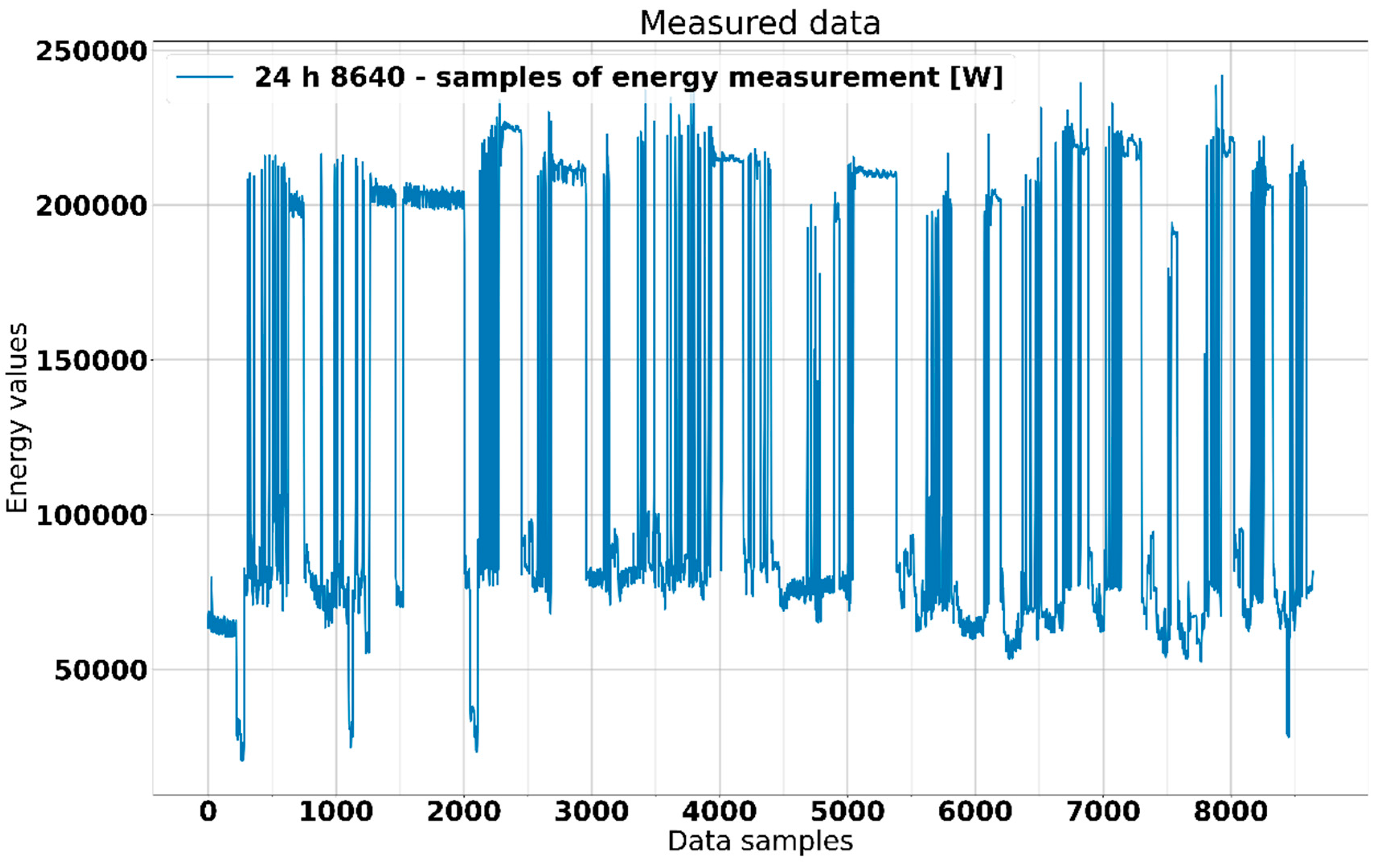
| Number of samples | 8640 |
| Mean value | 122,241.410 |
| Standard deviation | 64,964.959 |
| Minimum value | 20,386.545 |
| Maximum value | 241,949.547 |
| Q1 | 72,733.056 |
| Median | 82,668.418 |
| Q3 | 203,871.187 |
| Layer Type | Number of Units | Number of Params |
|---|---|---|
| LSTM | 128 | 66,560 |
| Danse | 1 | 129 |
| Total params | 66,689 | |
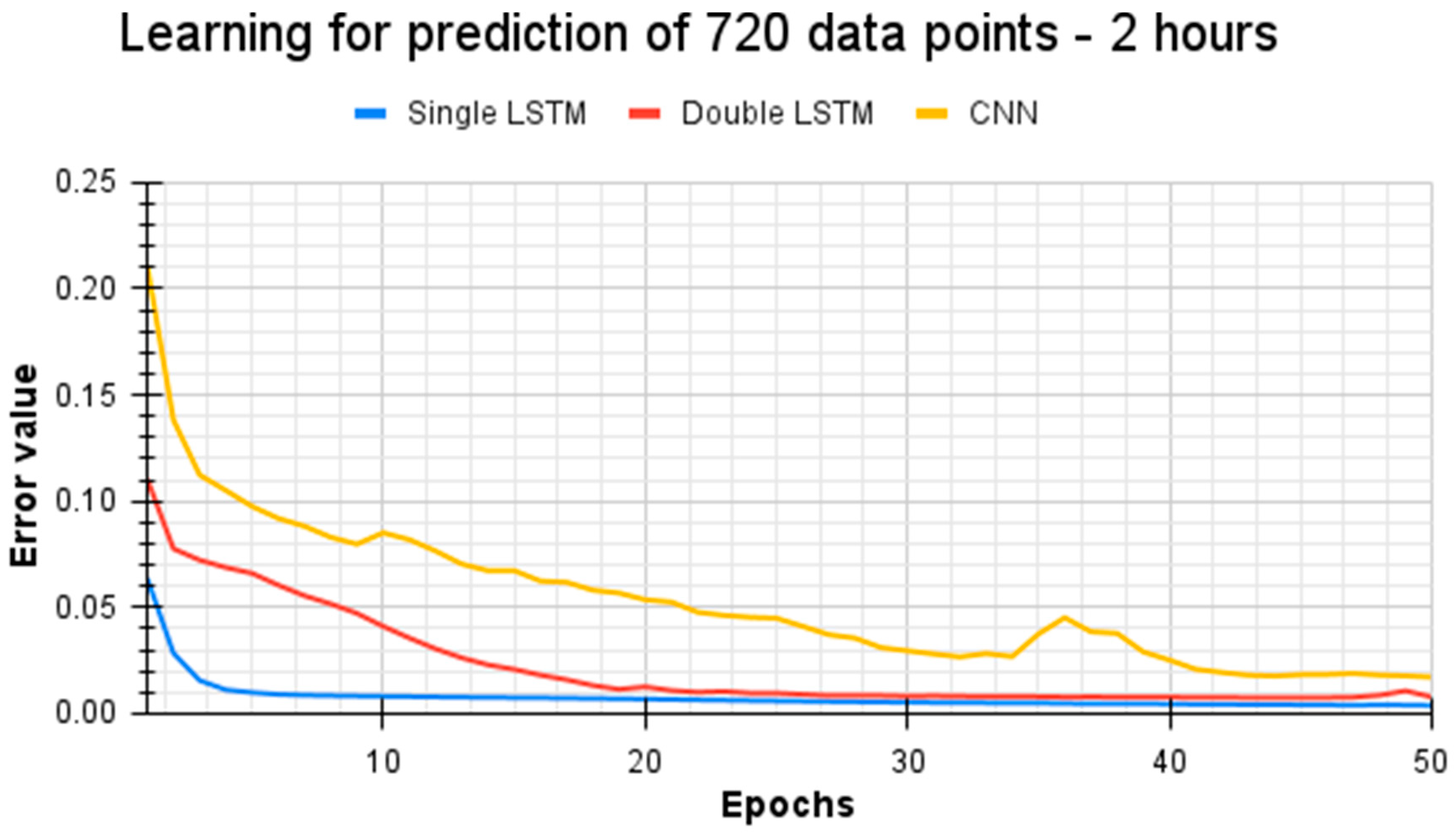
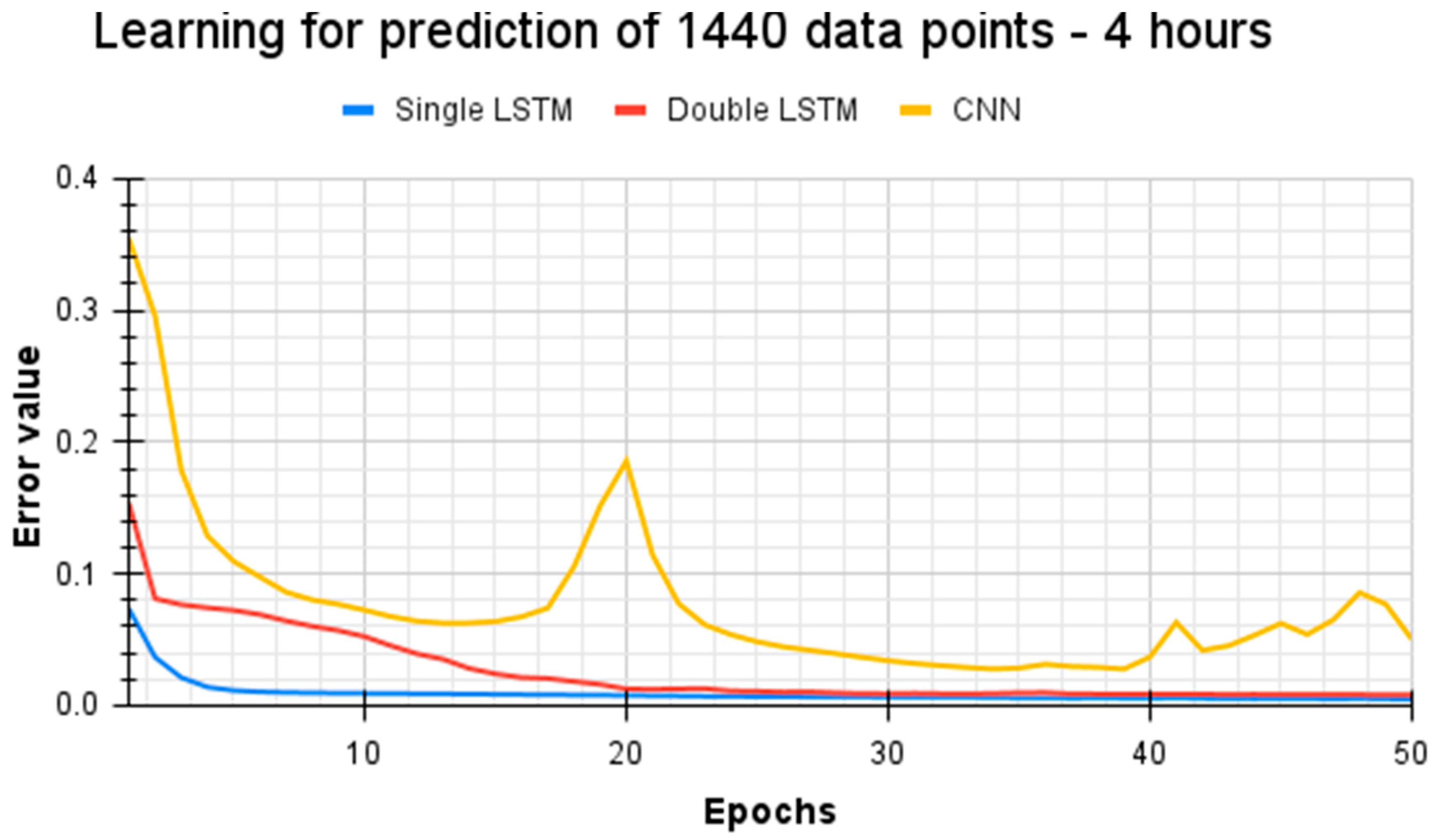
| Parameter | Prediction 1 h (360 Points) | Prediction 2 h (720 Points) | Prediction 3 h (1080 Points) | Prediction 4 h (1440 Points) | |
|---|---|---|---|---|---|
| 1 | Single-layer LSTM mean-squared error | 0.0112 | 0.0087 | 0.0084 | 0.0067 |
| 2 | Single-layer LSTM mean absolute error | 0.0524 | 0.0464 | 0.0487 | 0.0476 |
| 3 | Single-layer LSTM cosine similarity | 0.9039 | 0.9080 | 0.9195 | 0.9105 |
| 4 | Double-layer LSTM mean-squared error | 0.0119 | 0.0102 | 0.0111 | 0.0085 |
| 5 | Double-layer LSTM mean absolute error | 0.0714 | 0.0486 | 0.0494 | 0.0389 |
| 6 | Double-layer LSTM cosine similarity | 0.8565 | 0.9467 | 0.9588 | 0.9378 |
| 7 | CNN network mean-squared error | 0.0178 | 0.0497 | 0.1420 | 0.0885 |
| 8 | CNN network mean absolute error | 0.0844 | 0.1737 | 0.3272 | 0.2322 |
| 9 | CNN network cosine similarity | 0.8504 | 0.2058 | −0.32133 | 0.5397 |
| Models | Single-Layer LSTM | Double-Layer LSTM | CNN Layers |
|---|---|---|---|
| Single-layer LSTM | - | 0.70 | 0.99 |
| Double-Layer LSTM | 0.30 | - | 0.99 |
| CNN layers | <0.0001 | <0.0001 | - |
Publisher’s Note: MDPI stays neutral with regard to jurisdictional claims in published maps and institutional affiliations. |
© 2022 by the authors. Licensee MDPI, Basel, Switzerland. This article is an open access article distributed under the terms and conditions of the Creative Commons Attribution (CC BY) license (https://creativecommons.org/licenses/by/4.0/).
Share and Cite
Slowik, M.; Urban, W. Machine Learning Short-Term Energy Consumption Forecasting for Microgrids in a Manufacturing Plant. Energies 2022, 15, 3382. https://doi.org/10.3390/en15093382
Slowik M, Urban W. Machine Learning Short-Term Energy Consumption Forecasting for Microgrids in a Manufacturing Plant. Energies. 2022; 15(9):3382. https://doi.org/10.3390/en15093382
Chicago/Turabian StyleSlowik, Maciej, and Wieslaw Urban. 2022. "Machine Learning Short-Term Energy Consumption Forecasting for Microgrids in a Manufacturing Plant" Energies 15, no. 9: 3382. https://doi.org/10.3390/en15093382
APA StyleSlowik, M., & Urban, W. (2022). Machine Learning Short-Term Energy Consumption Forecasting for Microgrids in a Manufacturing Plant. Energies, 15(9), 3382. https://doi.org/10.3390/en15093382