
Emission Quantification via Passive Infrared Optical Gas Imaging: A Review


Abstract
:1. Introduction
2. Challenges in IOGI Emission Quantification
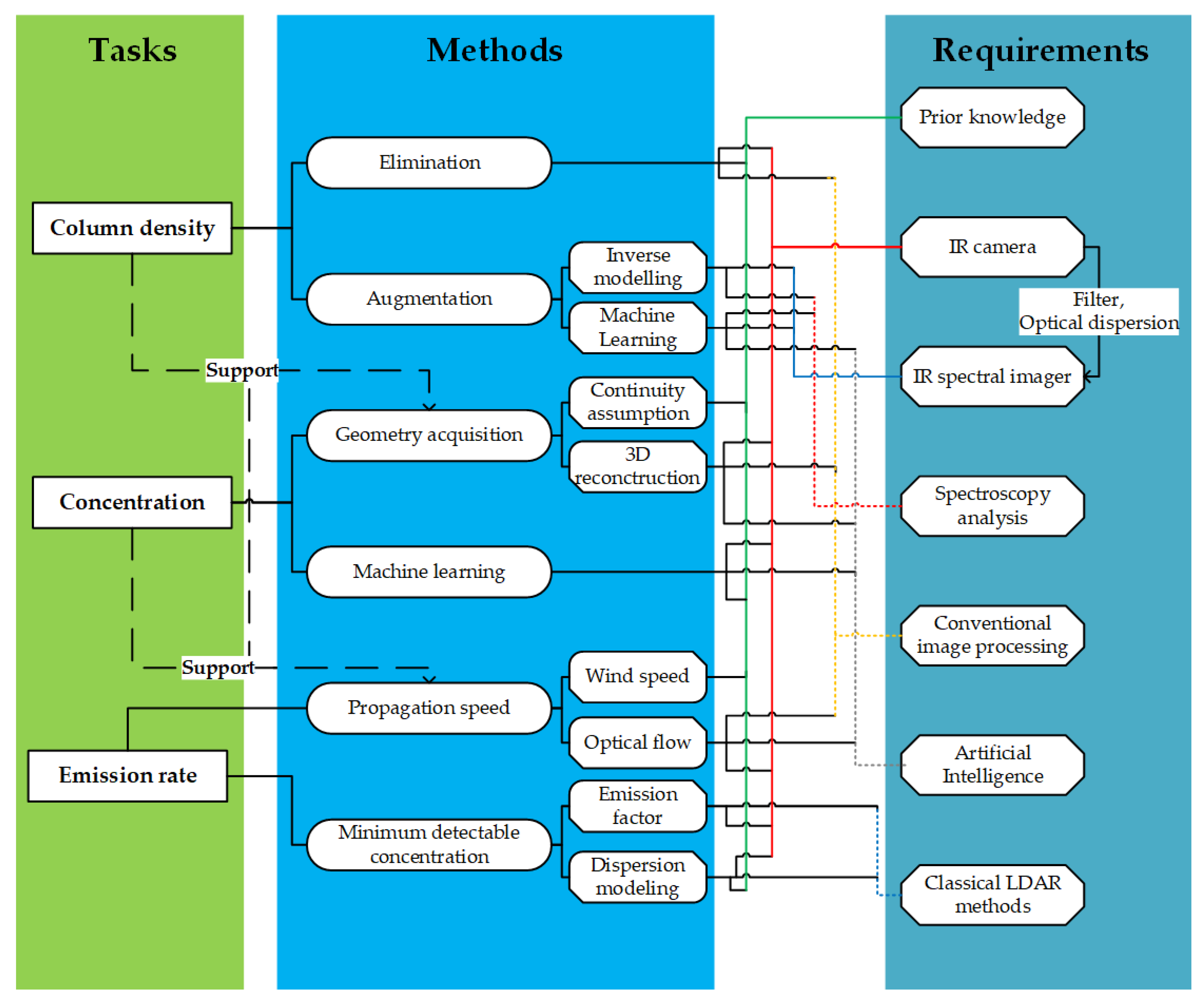
3. Column Density Quantification
3.1. Elimination Methods
3.2. Augmentation Methods
3.2.1. Inverse Modelling
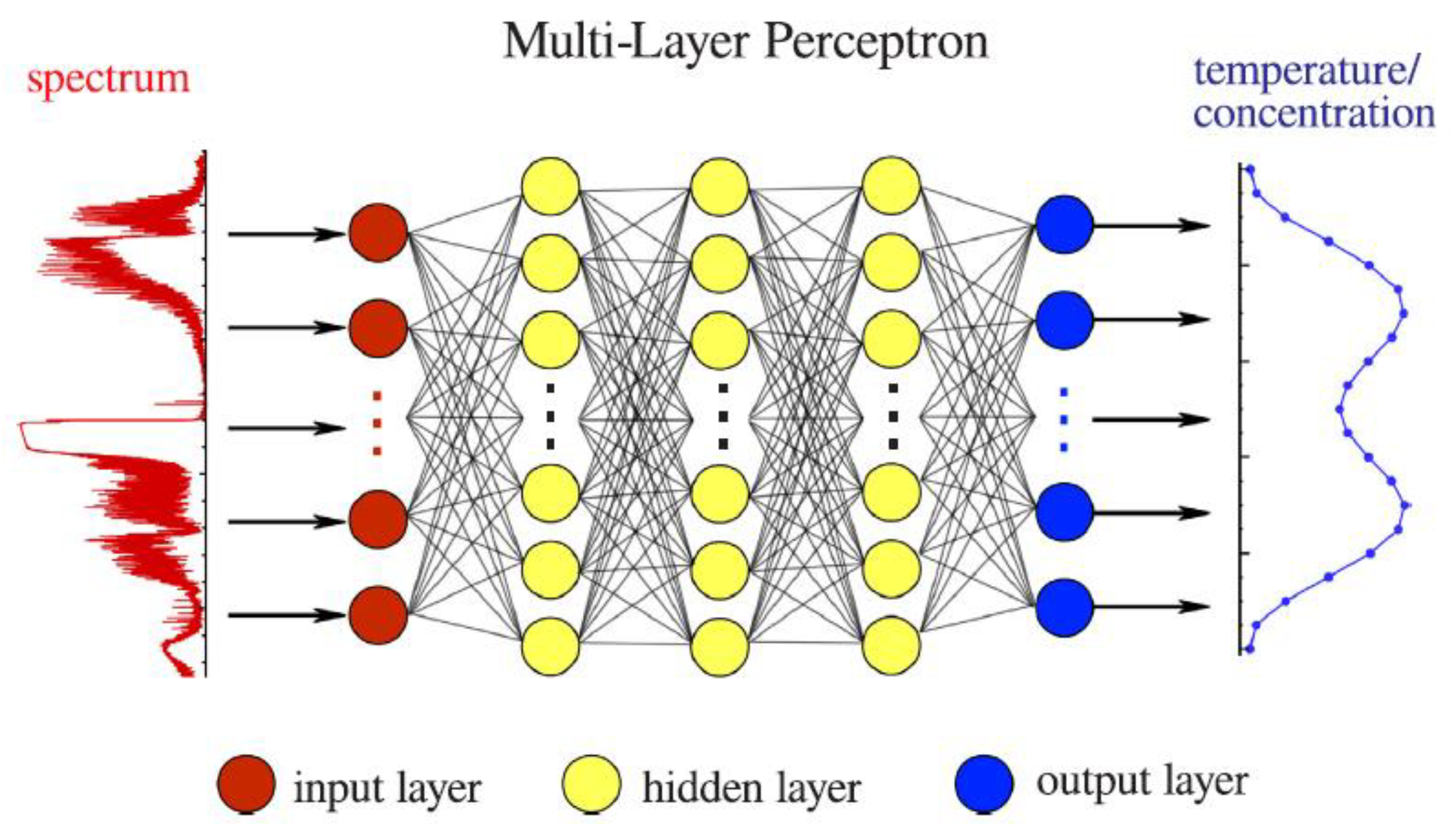
3.2.2. Machine-Learning-Based Methods
3.2.3. Hardware Limitations
3.3. A Comparison of Elimination and Augmentation Methods
- The need to generate lookup tables or fitting functions from calibrating massive combinations of temperature information, pixel values, and column density, which is time-consuming.
- The requirement for prior knowledge of temperature from ancillary devices, which raises the question of why not directly use ancillary devices instead of IOGI in order to quantify the emissions, such as all kinds of laser diagnostics.
- Acquisition of ancillary information requires access to the emission sites, which cancels the remote sensing advantage of IOGI.
- Since the infrared image captures black-body and rotational/vibrational emission from all molecules in the utilized bandwidth, in order to measure the column density of a specific molecule, a particular narrow-bandpass filter is necessary. The consequence is the elimination method cannot quantify several molecules simultaneously. On the contrary, because of the previous knowledge of spectral information, the augmentation method can avoid this weakness, as shown in Ren et al. [64].
4. Concentration Quantification
4.1. Geometry Acquisition-Based Methods
4.2. Machine-Learning-Based Methods
5. Emission Rate Quantification
5.1. Propagation-Speed-Based Method
5.2. Minimum-Detectable-Concentration-Based Method
6. Summary, Future Prospects, and Conclusions
- The advent of carbonless fuels and fuels of reduced carbon trace. It is serendipitous but also a matter of fact that such fuels (H2, NH3, light alcohols, and oxymethylethers), which are increasingly considered indispensable parts of the energy portfolio during the rapidly emerging energy transition, will generate flames and plumes that will have substantially less complicated spectroscopy, mainly due to the complete lack or the substantial decrease of soot and carbon oxides. The related fields of infrared emission can be very reasonably expected to be much simpler in terms of quantitative interpretation.
- The rapid progress in the field of AI algorithms, some of which can be transferred, as we showed above from other applications to IOGI. It is true that this explosive AI progress is on occasion non-uniform. For example, the machine learning algorithms applied in augmentation methods are still under development, while the machine learning algorithms used in 3D reconstruction or optical flow are very mature. It is our expectation that AI algorithms will be able to break through the constraints of their application specificity and heavy reliance on data. Transfer learning and meta-learning offer substantial hope on this front.
- The emergence of the “physics-guided” and “physics-discovered” AI [163,164,165,166]. Powerful algorithms directly transferred from the field of computer science can be strengthened substantially if the physics underlying the acquisition of IOGI data is coupled with the mathematics of machine learning. Currently, algorithms rely to a substantial extent on prior knowledge of several features of the solution, shown in this review. These requirements could possibly be alleviated if, e.g., the mathematics of the reactive flow could be embedded into the models or learnt from the data. Meanwhile, it is exciting that machine learning models can provide physical insights, which will, in turn, stimulate further developments in theory and the systems themselves, e.g., through the application of symbolic regression [167,168]. Further improvements in terms of IR-imaging hardware, such as sensitivity in the near-IR and availability of relatively cheap band-pass filters, will also provide a boost to IOGI technologies.
Author Contributions
Funding
Institutional Review Board Statement
Informed Consent Statement
Data Availability Statement
Conflicts of Interest
References
- Bell, J.N.B.; Honour, S.L.; Power, S.A. Effects of vehicle exhaust emissions on urban wild plant species. Environ. Pollut. 2011, 159, 1984–1990. [Google Scholar] [CrossRef] [PubMed]
- Brandt, A.R.; Heath, G.A.; Cooley, D. Methane Leaks from Natural Gas Systems Follow Extreme Distributions. Environ. Sci. Technol. 2016, 50, 12512–12520. [Google Scholar] [CrossRef] [PubMed]
- United Nations Secretary-General. Carbon Neutrality by 2050: The World’s Most Urgent Mission. Available online: https://www.un.org/sg/en/content/sg/articles/2020-12-11/carbon-neutrality-2050-the-world’s-most-urgent-mission (accessed on 15 February 2022).
- Vollmer, M.; Möllmann, K.-P. Infrared Thermal Imaging: Fundamentals, Research and Applications; John Wiley & Sons: Hoboken, NJ, USA, 2017. [Google Scholar]
- Tien, C.L.; Lee, S.C. Flame radiation. Prog. Energy Combust. Sci. 1982, 8, 41–59. [Google Scholar] [CrossRef]
- Bates, S.C.; Morrison, P.W., Jr.; Solomon, P.R. Infrared monitoring of combustion. In Proceedings of the Environmental Sensing and Combustion Diagnostics; Santoleri, J.J., Ed.; SPIE: Bellingham, WA, USA, 1991; Volume 1434, pp. 28–38. [Google Scholar]
- Rothman, L.S.; Gordon, I.E.; Barbe, A.; Benner, D.C.; Bernath, P.F.; Birk, M.; Boudon, V.; Brown, L.R.; Campargue, A.; Champion, J.-P.; et al. The HITRAN 2008 molecular spectroscopic database. J. Quant. Spectrosc. Radiat. Transf. 2009, 110, 533–572. [Google Scholar] [CrossRef] [Green Version]
- Ravikumar, A.P.; Wang, J.; Brandt, A.R. Are Optical Gas Imaging Technologies Effective for Methane Leak Detection? Environ. Sci. Technol. 2017, 51, 718–724. [Google Scholar] [CrossRef]
- Sabbah, S. Remote sensing of gases by hyperspectral imaging: System performance and measurements. Opt. Eng. 2012, 51, 111717. [Google Scholar] [CrossRef]
- Hinnrichs, M. Imaging spectrometer for fugitive gas leak detection. In Proceedings of the Imaging Spectrometer for Fugitive Gas Leak Detection; Vo-Dinh, T., Spellicy, R.L., Eds.; SPIE: Bellingham, WA, USA, 1999; Volume 3853, pp. 152–161. [Google Scholar]
- Burnett, J.D.; Wing, M.G. A low-cost near-infrared digital camera for fire detection and monitoring. Int. J. Remote Sens. 2018, 39, 741–753. [Google Scholar] [CrossRef]
- Katayama, H.; Naitoh, M.; Suganuma, M.; Harada, M.; Okamura, Y.; Tange, Y.; Nakau, K. Development of the Compact InfraRed Camera (CIRC) for wildfire detection. Remote Sens. Syst. Eng. II 2009, 7458, 745806. [Google Scholar] [CrossRef]
- Wu, J.; Wu, Z.; Ding, H.; Wei, Y.; Yang, X.; Li, Z.; Yang, B.R.; Liu, C.; Qiu, L.; Wang, X. Multifunctional and High-Sensitive Sensor Capable of Detecting Humidity, Temperature, and Flow Stimuli Using an Integrated Microheater. ACS Appl. Mater. Interfaces 2019, 11, 43383–43392. [Google Scholar] [CrossRef]
- Le Noc, L.; Dufour, D.; Terroux, M.; Tremblay, B.; Lambert, J.; Mercier, L.; Morissette, M.; Vachon, C.; Tang, D.; Bergeron, A. Towards very high-resolution infrared camera core. In Infrared Technology and Applications XXXVII; SPIE: Bellingham, WA, USA, 2011; Volume 8012, p. 80123. [Google Scholar] [CrossRef]
- Kohse-Höinghaus, K.; Jeffries, J.B. Applied Combustion Diagnostics; Taylor & Francis: New York, NY, USA, 2002. [Google Scholar]
- U.S. Environmental Protection Agency Technical Support Document Optical Gas Imaging Protocol. Available online: https://www.regulations.gov/document?D=EPA-HQ-OAR-2010-0505-4949 (accessed on 15 February 2022).
- U.S. Environmental Protection Agency. EPA Handbook: Optical Remote Sensing for Measurement and Monitoring of Emissions Flux; U.S. Environmental Protection Agency: Washington, DC, USA, 2011.
- De Almeida, P.; Correia, E.; Quintas, S. Detection and quantification of gas leakage by infrared technology in TEPA block 17 FPSOs. In Proceedings of the Society of Petroleum Engineers—SPE International Conference and Exhibition on Health, Safety, Environment, and Sustainability 2020, HSE Sustainability 2020, Virtual, 27–30 July 2020. [Google Scholar] [CrossRef]
- Lyman, S.N.; Tran, T.; Mansfield, M.L.; Ravikumar, A.P. Aerial and ground-based optical gas imaging survey of Uinta Basin oil and gas wells. Elementa 2019, 7, 43. [Google Scholar] [CrossRef]
- Furry, D.W.; Harris, G.; Ranum, D.; Anderson, E.P.; Carlstrom, V.M.; Sadik, W.A.; Shockley, C.E.; Siegell, J.H.; Smith, D.G. Evaluation of instrument leak detection capabilities for smart LDAR application: Refinery testing. Environ. Prog. Sustain. Energy 2009, 28, 273–284. [Google Scholar] [CrossRef]
- U.S. Environmental Protection Agency. Method 21—Volatile Organic Compound Leaks. Available online: https://www.epa.gov/emc/method-21-volatile-organic-compound-leaks (accessed on 15 February 2022).
- Lev-On, M.; Taback, H.; Epperson, D.; Siegell, J.; Gilmer, L.; Ritter, K. Methods for quantification of mass emissions from leaking process equipment when using optical imaging for leak detection. Environ. Prog. 2006, 25, 49–55. [Google Scholar] [CrossRef]
- U.S. Environmental Protection Agency. EPA Handbook: Optical and Remote Sensing for Measurement and Monitoring of Emissions Flux of Gases and Particulate Matter. Available online: https://www.epa.gov/sites/default/files/2018-08/documents/gd-52v.2.pdf (accessed on 15 February 2022).
- Fox, T.A.; Barchyn, T.E.; Risk, D.; Ravikumar, A.P.; Hugenholtz, C.H. A review of close-range and screening technologies for mitigating fugitive methane emissions in upstream oil and gas. Environ. Res. Lett. 2019, 14, 053002, Erratum in Environ. Res. Lett. 2019, 14, 069601. [Google Scholar] [CrossRef]
- Hagen, N. Survey of autonomous gas leak detection and quantification with snapshot infrared spectral imaging. J. Opt. 2020, 22, 103001. [Google Scholar] [CrossRef]
- Teledyne FLIR. Remote Tank Level Monitoring and Gas Detection with AI|Optical Gas Imaging|FLIR. Available online: https://www.youtube.com/watch?v=oNDg-cNTgMU (accessed on 15 February 2022).
- U.S. EPA Office of Air Quality Planning and Standards. Report for Oil and Natural Gas Sector Leaks; U.S. EPA Office of Air Quality Planning and Standards: Washington, DC, USA, 2014.
- Ravikumar, A.P.; Roda-Stuart, D.; Liu, R.; Bradley, A.; Bergerson, J.; Nie, Y.; Zhang, S.; Bi, X.; Brandt, A.R. Repeated leak detection and repair surveys reduce methane emissions over scale of years. Environ. Res. Lett. 2020, 15, 034029. [Google Scholar] [CrossRef]
- US Environmental Protection Agency. Protocol for Equipment Leak Emission Estimates; Office of Air Quality Planning and Standards: Research Triangle Park, NC, USA, 1995; p. 403.
- Connolly, J.I.; Robinson, R.A.; Gardiner, T.D. Assessment of the Bacharach Hi Flow® Sampler characteristics and potential failure modes when measuring methane emissions. Measurement 2019, 145, 226–233. [Google Scholar] [CrossRef]
- Al-hilal, H. Saudi Aramco Leak Detection and Repair (LDAR) Program. Available online: https://www.epa.gov/sites/default/files/2016-04/documents/tue6ldarprogram.pdf (accessed on 15 February 2022).
- Gal, F.; Kloppmann, W.; Proust, E.; Humez, P. Gas concentration and flow rate measurements as part of methane baseline assessment: Case of the Fontaine Ardente gas seep, Isère, France. Appl. Geochem. 2018, 95, 158–171. [Google Scholar] [CrossRef]
- Englander, J.G.; Brandt, A.R.; Conley, S.; Lyon, D.R.; Jackson, R.B. Aerial Interyear Comparison and Quantification of Methane Emissions Persistence in the Bakken Formation of North Dakota, USA. Environ. Sci. Technol. 2018, 52, 8947–8953. [Google Scholar] [CrossRef]
- Dierks, S.; Kroll, A. Quantification of methane gas leakages using remote sensing and sensor data fusion. In Proceedings of the SAS 2017—2017 IEEE Sensors Applications Symposium, Glassboro, NJ, USA, 13–15 March 2017. [Google Scholar] [CrossRef]
- Hagen, N.; Kester, R.T.; Walker, C. Real-time quantitative hydrocarbon gas imaging with the gas cloud imager (GCI). In Chemical, Biological, Radiological, Nuclear, and Explosives (CBRNE) Sensing XIII; SPIE: Bellingham, WA, USA, 2012; Volume 8358, p. 83581J. [Google Scholar] [CrossRef]
- Whiting, E.E. An empirical approximation to the Voigt profile. J. Quant. Spectrosc. Radiat. Transf. 1968, 8, 1379–1384. [Google Scholar] [CrossRef]
- Golowich, S.E.; Manolakis, D.G. Performance limits of LWIR gaseous plume quantification. In Algorithms and Technologies for Multispectral, Hyperspectral, and Ultraspectral Imagery XVII; SPIE: Bellingham, WA, USA, 2011; Volume 8048, p. 80481F. [Google Scholar] [CrossRef]
- Benson, R.G.; Panek, J.A.; Drayton, P. Direct Measurements of Minimum Detectable Vapor Concentrations Using Passive Infrared Optical Imaging Systems. In Proceedings of the AWMA Air Quality Measurements, Methods and Technology Symposium, Durham, NC, USA, 9–11 May 2006; p. 1025. [Google Scholar]
- Zeng, Y.; Morris, J. Calibration and Quantification Method for Gas Imaging Camera. U.S. Patent No. 9,325,915 B2, 26 April 2016. [Google Scholar]
- Zeng, Y.; Morris, J.; Sanders, A.; McGregor, D.; Kangas, P.; Abdel-Moati, H. New optical gas imaging technology for quantifying fugitive emission rates. In Proceedings of the Air and Waste Management Association’s Annual Conference and Exhibition AWMA 2015, Pittsburgh, PA, USA, 5–8 June 2017; Volume 3, pp. 2163–2168. [Google Scholar] [CrossRef]
- Sandsten, J.; Edner, H.; Svanberg, S. Gas imaging by infrared gas-correlation spectrometry. Opt. Lett. 1996, 21, 1945. [Google Scholar] [CrossRef] [Green Version]
- Wu, K.; Feng, Y.; Yu, G.; Liu, L.; Li, J.; Xiong, Y.; Li, F. Development of an imaging gas correlation spectrometry based mid-infrared camera for two-dimensional mapping of CO in vehicle exhausts. Opt. Express 2018, 26, 8239. [Google Scholar] [CrossRef] [PubMed]
- Sandsten, J.; Weibring, P.; Edner, H.; Svanberg, S. Real-time gas-correlation imaging employing thermal background radiation. Opt. Express 2000, 6, 92. [Google Scholar] [CrossRef] [PubMed] [Green Version]
- Sandsten, J.; Andersson, M. Volume flow calculations on gas leaks imaged with infrared gas-correlation. Opt. Express 2012, 20, 20318. [Google Scholar] [CrossRef] [PubMed]
- Brooks, F.J. GE Gas Turbine Performance Characteristics; GE Power Systems: Schenectady, NY, USA, 2000. [Google Scholar]
- Schultz, I.A.; Goldenstein, C.S.; Jeffries, J.B.; Hanson, R.K.; Rockwell, R.D.; Goyne, C.P. Spatially resolved water measurements in a scramjet combustor using diode laser absorption. J. Propuls. Power 2014, 30, 1551–1558. [Google Scholar] [CrossRef]
- Wang, Z.; Fu, P.; Chao, X. Laser Absorption Sensing Systems: Challenges, Modeling, and Design Optimization. Appl. Sci. 2019, 9, 2723. [Google Scholar] [CrossRef] [Green Version]
- Rodríguez-Conejo, M.A.; Meléndez, J. Hyperspectral quantitative imaging of gas sources in the mid-infrared. Appl. Opt. 2015, 54, 141. [Google Scholar] [CrossRef]
- Palaghita, T.I. Combustor Exhaust Temperature Nonuniformity Sensing Using Diode Laser Absorption. Ph.D. Thesis, Georgia Institute of Technology, Atlanta, GA, USA, 2007. [Google Scholar]
- Young, S.J.; Johnson, B.R.; Hackwell, J.A. An in-scene method for atmospheric compensation of thermal hyperspectral data. J. Geophys. Res. Atmos. 2002, 107, 1–20. [Google Scholar] [CrossRef]
- Kochanov, R.V.; Gordon, I.E.; Rothman, L.S.; Wcisło, P.; Hill, C.; Wilzewski, J.S. HITRAN Application Programming Interface (HAPI): A comprehensive approach to working with spectroscopic data. J. Quant. Spectrosc. Radiat. Transf. 2016, 177, 15–30. [Google Scholar] [CrossRef]
- Gross, K.C.; Bradley, K.C.; Perram, G.P. Remote identification and quantification of industrial smokestack effluents via imaging fourier-transform spectroscopy. Environ. Sci. Technol. 2010, 44, 9390–9397. [Google Scholar] [CrossRef]
- Niu, S.; Golowich, S.E.; Ingle, V.K.; Manolakis, D.G. New approach to remote gas-phase chemical quantification: Selected-band algorithm. Opt. Eng. 2013, 53, 021111. [Google Scholar] [CrossRef]
- Gallagher, N.B.; Wise, B.M.; Sheen, D.M. Estimation of trace vapor concentration-pathlength in plumes for remote sensing applications from hyperspectral images. Anal. Chim. Acta 2003, 490, 139–152. [Google Scholar] [CrossRef]
- Gittins, C.M. Detection and characterization of chemical vapor fugitive emissions by nonlinear optimal estimation: Theory and simulation. Appl. Opt. 2009, 48, 4545–4561. [Google Scholar] [CrossRef] [PubMed]
- Niu, S.; Golowich, S.E.; Manolakis, D.G. Algorithms for remote quantification of chemical plumes: A comparative study. In Algorithms and Technologies for Multispectral, Hyperspectral, and Ultraspectral Imagery XVIII; SPIE: Bellingham, WA, USA, 2012; Volume 8390, p. 83902I. [Google Scholar] [CrossRef]
- Ren, T.; Modest, M.F. Optical determination of temperature and species concentration for homogeneous turbulent gas medium. Int. J. Heat Mass Transf. 2015, 90, 1178–1187. [Google Scholar] [CrossRef] [Green Version]
- Ren, T.; Modest, M.F. Temperature profile inversion from CO2 spectral intensities through levenberg-marquardt optimization and tikhonov regularization. In Proceedings of the AIAA Aviation 2014—11th AIAA/ASME Joint Thermophysics and Heat Transfer Conference, Atlanta, GA, USA, 16–20 June 2014; pp. 1–9. [Google Scholar] [CrossRef]
- Grauer, S.J.; Conrad, B.M.; Miguel, R.B.; Daun, K.J. Gaussian model for emission rate measurement of heated plumes using hyperspectral data. J. Quant. Spectrosc. Radiat. Transf. 2018, 206, 125–134. [Google Scholar] [CrossRef]
- Kim, H.K.; Song, T.H. Determination of the gas temperature profile in a large-scale furnace using a fast/efficient inversion scheme for the SRS technique. J. Quant. Spectrosc. Radiat. Transf. 2005, 93, 369–381. [Google Scholar] [CrossRef]
- Liger, V.V.; Mironenko, V.R.; Kuritsyn, Y.A.; Bolshov, M.A. 2-T algorithm for temperature estimation in a non-uniform zone by line-of-site diode laser absorption spectroscopy. Laser Phys. Lett. 2019, 16, 125701. [Google Scholar] [CrossRef]
- Liger, V.V.; Mironenko, V.R.; Kuritsyn, Y.A.; Bolshov, M.A. Determination of the maximum temperature in a non-uniform hot zone by line-of-site absorption spectroscopy with a single diode laser. Sensors 2018, 18, 1608. [Google Scholar] [CrossRef] [Green Version]
- Liu, X.; Jeffries, J.B.; Hanson, R.K. Measurement of nonuniform temperature distributions using line-of-sight absorption spectroscopy. AIAA J. 2007, 45, 411–419. [Google Scholar] [CrossRef]
- Ren, T.; Modest, M.F.; Fateev, A.; Sutton, G.; Zhao, W.; Rusu, F. Machine learning applied to retrieval of temperature and concentration distributions from infrared emission measurements. Appl. Energy 2019, 252, 113448. [Google Scholar] [CrossRef] [Green Version]
- Song, T.H. Spectral remote sensing for furnaces and flames. Heat Transf. Eng. 2008, 29, 417–428. [Google Scholar] [CrossRef]
- Payan, S.; Hosseini Sarvari, S.M.; Behzadmehr, A. Inverse estimation of temperature profile in a non-gray medium with soot particles between two parallel plates. Numer. Heat Transf. Part A Appl. 2013, 63, 31–54. [Google Scholar] [CrossRef]
- Ouyang, T.; Wang, C.; Yu, Z.; Stach, R.; Mizaikoff, B.; Huang, G.-B.; Wang, Q.-J. NOx Measurements in Vehicle Exhaust Using Advanced Deep ELM Networks. IEEE Trans. Instrum. Meas. 2020, 70, 1. [Google Scholar] [CrossRef]
- Huang, G.B.; Zhu, Q.Y.; Siew, C.K. Extreme learning machine: Theory and applications. Neurocomputing 2006, 70, 489–501. [Google Scholar] [CrossRef]
- Gardner, M.; Dorling, S. Artificial neural networks (the multilayer perceptron)—A review of applications in the atmospheric sciences. Atmos. Environ. 1998, 32, 2627–2636. [Google Scholar] [CrossRef]
- Zhai, J.; Zhang, S.; Chen, J.; He, Q. Autoencoder and its various variants. In Proceedings of the 2018 IEEE International Conference on Systems, Man, and Cybernetics (SMC), Miyazaki, Japan, 7–10 October 2018; pp. 415–419. [Google Scholar]
- Noble, W.S. What is a support vector machine? Nat. Biotechnol. 2006, 24, 1565–1567. [Google Scholar] [CrossRef] [PubMed]
- Myles, A.J.; Feudale, R.N.; Liu, Y.; Woody, N.A.; Brown, S.D. An introduction to decision tree modeling. J. Chemom. J. Chemom. Soc. 2004, 18, 275–285. [Google Scholar] [CrossRef]
- Xie, T.; Yu, H.; Wilamowski, B. Comparison between traditional neural networks and radial basis function networks. In Proceedings of the 2011 IEEE International Symposium on Industrial Electronics, Gdansk, Poland, 27–30 June 2011; IEEE: Piscataway, NJ, USA, 2011; pp. 1194–1199. [Google Scholar]
- Goodfellow, I.; Bengio, Y.; Courville, A. Deep Learning; MIT Press: Cambridge, MA, USA, 2016. [Google Scholar]
- Vaswani, A.; Shazeer, N.; Parmar, N.; Uszkoreit, J.; Jones, L.; Gomez, A.N.; Kaiser, L.; Polosukhin, I. Attention Is All You Need. In Proceedings of the Advances in Neural Information Processing Systems, Long Beach, CA, USA, 4–9 December 2017; pp. 5999–6009. [Google Scholar]
- Han, K.; Wang, Y.; Chen, H.; Chen, X.; Guo, J.; Liu, Z.; Tang, Y.; Xiao, A.; Xu, C.; Xu, Y.; et al. A Survey on Vision Transformer. IEEE Trans. Pattern Anal. Mach. Intell. 2022. online ahead of print. [Google Scholar] [CrossRef]
- Zheng, A.; Casari, A. Feature Engineering for Machine Learning: Principles and Techniques for Data Scientists; O’Reilly Media, Inc.: Sebastopol, CA, USA, 2018; ISBN 1491953241. [Google Scholar]
- Fowler, J.E. Compressive pushbroom and whiskbroom sensing for hyperspectral remote-sensing imaging. In Proceedings of the 2014 IEEE International Conference on Image Processing (ICIP), Paris, France, 27–30 October 2014; IEEE: Piscataway, NJ, USA, 2014; pp. 684–688. [Google Scholar]
- Gat, N. Imaging spectroscopy using tunable filters: A review. Proc. Clin. Appl. Adult Attach. Interview 2000, 4056, 50–64. [Google Scholar]
- Hinnrichs, M.; Schmehl, R.; McCrigler, L.; Burke, P.; Engberg, A.; Buttini, P.; Donato, G.; Maggini, R. Infrared gas imaging and quantification camera for LDAR applications. In Proceedings of the Air & Waste Management Association—Mini-Symposium on Smart Leak Detection and Repair 2006, A WMA’s 99th Annual Conference & Exhibition, New Orleans, LA, USA, 20–23 June 2006; Volume 152 CP, pp. 380–404. [Google Scholar]
- Lewis, E.N.; Levin, I.W.; Treado, P.J.; Reeder, R.C.; Story, G.M.; Dowrey, A.E.; Marcott, C. Fourier Transform Spectroscopic Imaging Using an Infrared Focal-Plane Array Detector. Anal. Chem. 1995, 67, 3377–3381. [Google Scholar] [CrossRef]
- Hagen, N. Snapshot advantage: A review of the light collection improvement for parallel high-dimensional measurement systems. Opt. Eng. 2012, 51, 111702. [Google Scholar] [CrossRef]
- Eckbreth, A.C. Laser Diagnostics for Combustion Temperature and Species; CRC Press: Boca Raton, FL, USA, 1996; Volume 3. [Google Scholar]
- Hagen, N.; Kudenov, M.W. Review of snapshot spectral imaging technologies. Opt. Eng. 2013, 52, 090901. [Google Scholar] [CrossRef] [Green Version]
- Hagen, N.; Kester, R.T.; Morlier, C.G.; Panek, J.A.; Drayton, P.; Fashimpaur, D.; Stone, P.; Adams, E. Video-rate spectral imaging of gas leaks in the longwave infrared. In Chemical, Biological, Radiological, Nuclear, and Explosives (CBRNE) Sensing XIV; SPIE: Bellingham, WA, USA, 2013; Volume 8710, p. 871005. [Google Scholar] [CrossRef]
- Willson, B. Methane Quantification & ARPA-E’s MONITOR Program. Available online: https://www.epa.gov/sites/default/files/2016-04/documents/21willson.pdf (accessed on 15 February 2022).
- Bell, C.S.; Vaughn, T.; Zimmerle, D. Evaluation of next generation emission measurement technologies under repeatable test protocols. Elem. Sci. Anthr. 2020, 8, 32. [Google Scholar] [CrossRef]
- Singh, D.; Barlow, B.; Hugenholtz, C.; Funk, W.; Ravikumar, A. Field Trial of New Methane Detection Technologies: Results from the Alberta Methane Field Challenge. ESNT—Eng. 2020. in prep. [Google Scholar] [CrossRef]
- Buckland, K.N.; Young, S.J.; Keim, E.R.; Johnson, B.R.; Johnson, P.D.; Tratt, D.M. Tracking and quantification of gaseous chemical plumes from anthropogenic emission sources within the Los Angeles Basin. Remote Sens. Environ. 2017, 201, 275–296. [Google Scholar] [CrossRef]
- Rhoby, M.R.; Blunck, D.L.; Gross, K.C. Mid-IR hyperspectral imaging of laminar flames for 2-D scalar values. Opt. Express 2014, 22, 21600. [Google Scholar] [CrossRef]
- Harley, J.L.; Rolling, A.J.; Wisniewski, C.F.; Gross, K.C. Spatially resolved infrared spectra of F109 turbofan exhaust. In Thermosense: Thermal Infrared Applications XXXIV; SPIE: Bellingham, WA, USA, 2012; Volume 8354, p. 83540H. [Google Scholar] [CrossRef]
- Naranjo, E.; Baliga, S.; Bernascolle, P. IR gas imaging in an industrial setting. In Thermosense XXXII; SPIE: Bellingham, WA, USA, 2010; Volume 7661, p. 76610K. [Google Scholar] [CrossRef]
- THORLABS Motorized Fast-Change Filter Wheel. Available online: https://www.thorlabs.com/newgrouppage9.cfm?objectgroup_id=2945 (accessed on 15 February 2022).
- Luo, X.; Ma, J.; Chen, D.; Wang, L.; Cai, Y.; Huang, P.; Wang, C.; Luo, H.; Xue, W. Archimedean spiral push-broom differential thermal imaging for gas leakage detection. Opt. Express 2019, 27, 9099. [Google Scholar] [CrossRef]
- Brauers, J.; Schulte, N.; Aach, T. Multispectral Filter-Wheel Cameras: Geometric Distortion Model and Compensation Algorithms. IEEE Trans. Image Process. 2008, 17, 2368–2380. [Google Scholar] [CrossRef]
- Krabicka, J.; Lu, G.; Yan, Y. Profiling and characterization of flame radicals by combining spectroscopic imaging and neural network techniques. IEEE Trans. Instrum. Meas. 2011, 60, 1854–1860. [Google Scholar] [CrossRef]
- Yang, J.; Lin, P.T. Real-time and non-destructive gas mixture analysis using linear various filter enabled mid-infrared visualization. Opt. Express 2019, 27, 26512. [Google Scholar] [CrossRef]
- Olbrycht, R.; Kałuża, M.; Wittchen, W.; Borecki, M.; Więcek, B.; De Mey, G.; Kopeć, M. Gas identification and estimation of its concentration in a tube using thermographic camera with diffraction grating. Quant. Infrared Thermogr. J. 2018, 15, 106–120. [Google Scholar] [CrossRef]
- Ko, B.; Jung, J.H.; Nam, J.Y. Fire detection and 3D surface reconstruction based on stereoscopic pictures and probabilistic fuzzy logic. Fire Saf. J. 2014, 68, 61–70. [Google Scholar] [CrossRef]
- Rossi, L.; Akhloufi, M.; Tison, Y. On the use of stereovision to develop a novel instrumentation system to extract geometric fire fronts characteristics. Fire Saf. J. 2011, 46, 9–20. [Google Scholar] [CrossRef]
- Rangel, J.; Kroll, A. Characterization and calibration of a stereo gas camera system for obtaining spatial information of gas structures. In Proceedings of the 2018 IEEE Sensors Applications Symposium SAS 2018, Seoul, Korea, 12–14 March 2018; pp. 1–6. [Google Scholar] [CrossRef]
- Rossi, L.; Molinier, T.; Akhloufi, M.; Tison, Y.; Pieri, A. A 3D vision system for the measurement of the rate of spread and the height of fire fronts. Meas. Sci. Technol. 2010, 21, 105501. [Google Scholar] [CrossRef]
- Ma, Z.; Liu, S. A review of 3D reconstruction techniques in civil engineering and their applications. Adv. Eng. Inform. 2018, 37, 163–174. [Google Scholar] [CrossRef]
- Han, X.F.; Laga, H.; Bennamoun, M. Image-based 3d object reconstruction: State-of-the-art and trends in the deep learning era. IEEE Trans. Pattern Anal. Mach. Intell. 2021, 43, 1578–1604. [Google Scholar] [CrossRef] [Green Version]
- Schofield, R.; King, L.; Tayal, U.; Castellano, I.; Stirrup, J.; Pontana, F.; Earls, J.; Nicol, E. Image reconstruction: Part 1—Understanding filtered back projection, noise and image acquisition. J. Cardiovasc. Comput. Tomogr. 2020, 14, 219–225. [Google Scholar] [CrossRef]
- Willemink, M.J.; De Jong, P.A.; Leiner, T.; De Heer, L.M.; Nievelstein, R.A.J.; Budde, R.P.J.; Schilham, A.M.R. Iterative reconstruction techniques for computed tomography Part 1: Technical principles. Eur. Radiol. 2013, 23, 1623–1631. [Google Scholar] [CrossRef]
- Cai, W.; Kaminski, C.F. Tomographic absorption spectroscopy for the study of gas dynamics and reactive flows. Prog. Energy Combust. Sci. 2017, 59, 1–31. [Google Scholar] [CrossRef]
- De Donato, P.; Barres, O.; Sausse, J.; Taquet, N. Advances in 3-D infrared remote sensing gas monitoring. application to an urban atmospheric environment. Remote Sens. Environ. 2016, 175, 301–309. [Google Scholar] [CrossRef]
- Watremez, X.; Labat, N.; Audouin, G.; Lejay, B.; Marcarian, X.; Dubucq, D.; Marblé, A.; Foucher, P.Y.; Poutier, L.; Danno, R.; et al. Remote detection and flow rates quantification of methane releases using infrared camera technology and 3D reconstruction algorithm. In Proceedings of the SPE Annual Technical Conference and Exhibition 2016, Dubai, United Arab Emirates, 26–28 September 2016; pp. 1–17. [Google Scholar] [CrossRef]
- Tancin, R.J.; Spearrin, R.M.; Goldenstein, C.S. 2D mid-infrared laser-absorption imaging for tomographic reconstruction of temperature and carbon monoxide in laminar flames. Opt. Express 2019, 27, 14184. [Google Scholar] [CrossRef]
- Yu, T.; Cai, W. Benchmark evaluation of inversion algorithms for tomographic absorption spectroscopy. Appl. Opt. 2017, 56, 2183. [Google Scholar] [CrossRef] [PubMed]
- Cai, W.; Liu, H.; Huang, J.; Zhang, J. Reconstruction of kHz-rate 3-D flame image sequences from a low-rate 2-D recording via a data-driven approach. J. Opt. Soc. Am. B 2020, 37, 3564. [Google Scholar] [CrossRef]
- Huang, J.; Liu, H.; Cai, W. Tomographic reconstruction for 3D flame imaging using convolutional neural networks. In Proceedings of the 12th Asia-Pacific Conference on Combustion ASPACC 2019, Fukuoka, Japan, 1–5 July 2019; pp. 3–6. [Google Scholar]
- Huang, J.; Liu, H.; Wang, Q.; Cai, W. Limited-projection volumetric tomography for time-resolved turbulent combustion diagnostics via deep learning. Aerosp. Sci. Technol. 2020, 106, 106123. [Google Scholar] [CrossRef]
- Deng, A.; Huang, J.; Liu, H.; Cai, W. Deep learning algorithms for temperature field reconstruction of nonlinear tomographic absorption spectroscopy. Meas. Sens. 2020, 10–12, 100024. [Google Scholar] [CrossRef]
- Huang, J.; Liu, H.; Dai, J.; Cai, W. Reconstruction for limited-data nonlinear tomographic absorption spectroscopy via deep learning. J. Quant. Spectrosc. Radiat. Transf. 2018, 218, 187–193. [Google Scholar] [CrossRef]
- Huang, J.; Zhao, J.; Cai, W. Compressing convolutional neural networks using POD for the reconstruction of nonlinear tomographic absorption spectroscopy. Comput. Phys. Commun. 2019, 241, 33–39. [Google Scholar] [CrossRef]
- Huang, J.; Liu, H.; Cai, W. Online in situ prediction of 3-D flame evolution from its history 2-D projections via deep learning. J. Fluid Mech. 2019, 875, R2. [Google Scholar] [CrossRef]
- Wei, C.; Schwarm, K.K.; Pineda, D.I.; Spearrin, R.M. Deep neural network inversion for 3D laser absorption imaging of methane in reacting flows. Opt. Lett. 2020, 45, 2447. [Google Scholar] [CrossRef]
- Hochreiter, S.; Schmidhuber, J. Long Short-Term Memory. Neural Comput. 1997, 9, 1735–1780. [Google Scholar] [CrossRef]
- Salakhutdinov, R.; Murray, I. On the quantitative analysis of deep belief networks. In Proceedings of the 25th International Conference on Machine Learning, Helsinki, Finland, 5–9 July 2008; pp. 872–879. [Google Scholar] [CrossRef] [Green Version]
- Jiang, H.; Sun, D.; Jampani, V.; Yang, M.H.; Learned-Miller, E.; Kautz, J. Super SloMo: High Quality Estimation of Multiple Intermediate Frames for Video Interpolation. In Proceedings of the IEEE Computer Society Conference on Computer Vision and Pattern Recognition, Salt Lake City, UT, USA, 18–23 June 2018; pp. 9000–9008. [Google Scholar] [CrossRef] [Green Version]
- Rodríguez, A.; Escudero, F.; Cruz, J.J.; Carvajal, G.; Fuentes, A. Retrieving soot volume fraction fields for laminar axisymmetric diffusion flames using convolutional neural networks. Fuel 2021, 285, 119011. [Google Scholar] [CrossRef]
- Chen, J.; Chan, L.L.T.; Cheng, Y.C. Gaussian process regression based optimal design of combustion systems using flame images. Appl. Energy 2013, 111, 153–160. [Google Scholar] [CrossRef]
- Li, N.; Lu, G.; Li, X.; Yan, Y. Prediction of NOx emissions from a biomass fired combustion process through digital imaging, non-negative matrix factorization and fast sparse regression. In Proceedings of the IEEE Instrumentation and Measurement Technology Conference, Pisa, Italy, 11–14 May 2015; pp. 176–180. [Google Scholar] [CrossRef]
- Li, N.; Lu, G.; Li, X.; Yan, Y. Prediction of Pollutant Emissions of Biomass Flames Through Digital Imaging, Contourlet Transform, and Support Vector Regression Modeling. IEEE Trans. Instrum. Meas. 2015, 64, 2409–2416. [Google Scholar] [CrossRef]
- Liu, Y.; Fan, Y.; Chen, J. Flame Images for Oxygen Content Prediction of Combustion Systems Using DBN. Energy Fuels 2017, 31, 8776–8783. [Google Scholar] [CrossRef]
- Ögren, Y.; Tóth, P.; Garami, A.; Sepman, A.; Wiinikka, H. Development of a vision-based soft sensor for estimating equivalence ratio and major species concentration in entrained flow biomass gasification reactors. Appl. Energy 2018, 226, 450–460. [Google Scholar] [CrossRef]
- Golgiyaz, S.; Talu, M.F.; Onat, C. Artificial neural network regression model to predict flue gas temperature and emissions with the spectral norm of flame image. Fuel 2019, 255, 115827. [Google Scholar] [CrossRef]
- González-Espinosa, A.; Gil, A.; Royo-Pascual, L.; Nueno, A.; Herce, C. Effects of hydrogen and primary air in a commercial partially-premixed atmospheric gas burner by means of optical and supervised machine learning techniques. Int. J. Hydrogen Energy 2020, 45, 31130–31150. [Google Scholar] [CrossRef]
- Rasmussen, C.E. Gaussian processes in machine learning. In Proceedings of the Summer School on Machine Learning, Canberra Australia, 4–16 August 2003; pp. 63–71. [Google Scholar]
- Ringnér, M. What is principal component analysis? Nat. Biotechnol. 2008, 26, 303–304. [Google Scholar] [CrossRef]
- Ronneberger, O.; Fischer, P.; Brox, T. U-Net: Convolutional Networks for Biomedical Image Segmentation. IEEE Access 2015, 9, 234–241. [Google Scholar]
- Pan, S.J.; Yang, Q. A survey on transfer learning. IEEE Trans. Knowl. Data Eng. 2010, 22, 1345–1359. [Google Scholar] [CrossRef]
- Hospedales, T.; Antoniou, A.; Micaelli, P.; Storkey, A. Meta-Learning in Neural Networks: A Survey. arXiv 2020, arXiv:2004.05439. [Google Scholar] [CrossRef]
- Parisi, G.I.; Kemker, R.; Part, J.L.; Kanan, C.; Wermter, S. Continual lifelong learning with neural networks: A review. Neural Netw. 2019, 113, 54–71. [Google Scholar] [CrossRef] [PubMed]
- Sherwin, E.D.; Chen, Y.; Ravikumar, A.P.; Brandt, A.R. Single-blind test of airplane-based hyperspectral methane detection via controlled releases. Elementa 2021, 9, 1–10. [Google Scholar] [CrossRef]
- Branson, K.; Jones, B.B.; Berman, E.S.F. Methane Emissions Quantification. Available online: https://kairosaerospace.com/wp-content/uploads/2020/05/Kairos-Emissions-Quantification.pdf (accessed on 20 February 2022).
- Horn, B.K.; Schunck, B.G. Determine Optical Flow. In Techniques and Applications of Image Understanding, Proceedings of the 1981 Technical Symposium East, Washington, DC, USA, 21–22 April 1981; Pearson, J.J., Ed.; SPIE: Bellingham, WA, USA, 1981; Volume 0281, pp. 319–331. [Google Scholar]
- Nagorski, M.; Miguel, R.B.; Talebi-Moghaddam, S.; Conrad, B.; Daun, K.J.; Nagorski, M.; Miguel, R.B.; Talebi-Moghaddam, S.; Conrad, B.; Daun, K.J. Velocimetry of Methane Emissions using Optical Gas Imaging. Available online: http://www.flarenet.ca/wp-content/uploads/2020/11/396970_PTAC-2020-Poster.pdf (accessed on 20 February 2022).
- Lucas, B.D.; Kanade, T. Iterative Image Registration Technique with an Application to Stereo Vision. In Proceedings of the DARPA Image Understanding Workshop, April 1981; Volume 2, pp. 121–130. [Google Scholar]
- Tokumaru, P.T.; Dimotakis, P.E. Image correlation velocimetry. Exp. Fluids 1995, 19, 1–15. [Google Scholar] [CrossRef] [Green Version]
- Rangel, J.; Schmoll, R.; Kroll, A. On scene flow computation of gas structures with optical gas imaging cameras. In Proceedings of the 2020 IEEE Winter Conference on Applications of Computer Vision (WACV) 2020, Snowmass, CO, USA, 1–5 March 2020; pp. 174–182. [Google Scholar] [CrossRef]
- Brox, T.; Bruhn, A.; Papenberg, N.; Weickert, J. High Accuracy Optical Flow Estimation Based on a Theory for Warping; Lecture Notes in Computer Science (including Subser. Lect. Notes Artif. Intell. Lect. Notes Bioinformatics); Springer: Berlin/Heidelberg, Germany, 2004; Volume 3024, pp. 25–36. [Google Scholar] [CrossRef]
- Harley, J.L.; Gross, K.C. Remote quantification of smokestack effluent mass flow rates using imaging Fourier transform spectrometry. In Chemical, Biological, Radiological, Nuclear, and Explosives (CBRNE) Sensing XII; SPIE: Bellingham, WA, USA, 2011; Volume 8018, p. 801813. [Google Scholar] [CrossRef]
- Dosovitskiy, A.; Fischery, P.; Ilg, E.; Hausser, P.; Hazirbas, C.; Golkov, V.; Van Der Smagt, P.; Cremers, D.; Brox, T. FlowNet: Learning optical flow with convolutional networks. In Proceedings of the IEEE International Conference on Computer Vision 2015, Santiago, Chile, 7–13 December 2015; pp. 2758–2766. [Google Scholar] [CrossRef] [Green Version]
- Meister, S.; Hur, J.; Roth, S. UnFlow: Unsupervised learning of optical flow with a bidirectional census loss. In Proceedings of the 32nd AAAI Conference on Artificial Intelligence AAAI 2018, New Orleans, CA, USA, 2–7 February 2018; pp. 7251–7259. [Google Scholar]
- Fortun, D.; Bouthemy, P.; Kervrann, C. Optical flow modeling and computation: A survey. Comput. Vis. Image Underst. 2015, 134, 1–21. [Google Scholar] [CrossRef] [Green Version]
- Tu, Z.; Xie, W.; Zhang, D.; Poppe, R.; Veltkamp, R.C.; Li, B.; Yuan, J. A survey of variational and CNN-based optical flow techniques. Signal Process. Image Commun. 2019, 72, 9–24. [Google Scholar] [CrossRef]
- Lev-On, M.; Epperson, D.; Siegell, J.; Ritter, K. Derivation of new emission factors for quantification of mass emissions when using optical gas imaging for detecting leaks. J. Air Waste Manag. Assoc. 2007, 57, 1061–1070. [Google Scholar] [CrossRef] [Green Version]
- Safitri, A.; Gao, X.; Mannan, M.S. Dispersion modeling approach for quantification of methane emission rates from natural gas fugitive leaks detected by infrared imaging technique. J. Loss Prev. Process Ind. 2011, 24, 138–145. [Google Scholar] [CrossRef]
- Thoma, E.D.; Brantley, H.; Squier, B.; DeWees, J.; Segall, R.; Merrill, R. Development of mobile measurement method series OTM 33. In Proceedings of the 108th Annual Conference of the Air & Waste Management Association, Raleigh, NC, USA, 22–25 June 2015; Air and Waste Management Association: Raleigh, NC, USA, 2015; Volume 2, pp. 921–935. [Google Scholar]
- Korsakissok, I.; Mallet, V. Comparative study of Gaussian dispersion formulas within the polyphemus platform: Evaluation with Prairie Grass and Kincaid experiments. J. Appl. Meteorol. Climatol. 2009, 48, 2459–2473. [Google Scholar] [CrossRef] [Green Version]
- Jain, A.; Sharma, A.; Borana, S.L.; Ravindra, B.; Mangalhara, J.P. Study and analysis of exhaust emission of diesel vehicles using thermal IR imagers. Def. Sci. J. 2018, 68, 533–539. [Google Scholar] [CrossRef] [Green Version]
- Blinke, J. Diffusion of Sustainable Innovations: A Case Study of Optical Gas Imaging; KTH Royal Institute of Technology: Stockholm, Sweden, 2020. [Google Scholar]
- Ravikumar, A.P.; Wang, J.; McGuire, M.; Bell, C.S.; Zimmerle, D.; Brandt, A.R. “Good versus Good Enough?” Empirical Tests of Methane Leak Detection Sensitivity of a Commercial Infrared Camera. Environ. Sci. Technol. 2018, 52, 2368–2374. [Google Scholar] [CrossRef]
- Stovern, M.; Murray, J.; Schwartz, C.; Beeler, C.; Thoma, E.D. Understanding oil and gas pneumatic controllers in the Denver–Julesburg basin using optical gas imaging. J. Air Waste Manag. Assoc. 2020, 70, 468–480. [Google Scholar] [CrossRef] [PubMed]
- Pacsi, A.P.; Ferrara, T.; Schwan, K.; Tupper, P.; Lev-On, M.; Smith, R.; Ritter, K. Equipment leak detection and quantification at 67 oil and gas sites in the Western United States. Elementa 2019, 7, 29. [Google Scholar] [CrossRef] [Green Version]
- Zimmerle, D.; Vaughn, T.; Bell, C.; Bennett, K.; Deshmukh, P.; Thoma, E. Detection Limits of Optical Gas Imaging for Natural Gas Leak Detection in Realistic Controlled Conditions. Environ. Sci. Technol. 2020, 54, 11506–11514. [Google Scholar] [CrossRef] [PubMed]
- Hagen, N. Sensitivity limits on optical gas imaging due to air turbulence. Opt. Eng. 2018, 57, 1. [Google Scholar] [CrossRef] [Green Version]
- Linne, M.A. Spectroscopic Measurement: An Introduction to the Fundamentals; Academic Press: Cambridge, MA, USA, 2002. [Google Scholar]
- Miguel, R.B.; Emmert, J.; Grauer, S.J.; Thornock, J.N.; Daun, K.J. Optimal filter selection for quantitative gas mixture imaging. J. Quant. Spectrosc. Radiat. Transf. 2020, 254, 107208. [Google Scholar] [CrossRef]
- Raissi, M.; Perdikaris, P.; Karniadakis, G.E. Physics-informed neural networks: A deep learning framework for solving forward and inverse problems involving nonlinear partial differential equations. J. Comput. Phys. 2019, 378, 686–707. [Google Scholar] [CrossRef]
- Muralidhar, N.; Islam, M.R.; Marwah, M.; Karpatne, A.; Ramakrishnan, N. Incorporating Prior Domain Knowledge into Deep Neural Networks. In Proceedings of the 2018 IEEE International Conference on Big Data (Big Data), Seattle, WA, USA, 10–13 December 2018; 2019; pp. 36–45. [Google Scholar] [CrossRef]
- Vonrueden, L.; Mayer, S.; Beckh, K.; Georgiev, B.; Giesselbach, S.; Heese, R.; Kirsch, B.; Walczak, M.; Pfrommer, J.; Pick, A.; et al. Informed Machine Learning—A Taxonomy and Survey of Integrating Prior Knowledge into Learning Systems. IEEE Trans. Knowl. Data Eng. 2021. early access. [Google Scholar] [CrossRef]
- Cranmer, M.; Sanchez-Gonzalez, A.; Battaglia, P.; Xu, R.; Cranmer, K.; Spergel, D.; Ho, S. Discovering symbolic models from deep learning with inductive biases. In Proceedings of the Advances in Neural Information Processing Systems 33: Annual Conference on Neural Information Processing Systems 2020, Virtual, 6–12 December 2020; pp. 1–25. [Google Scholar]
- Udrescu, S.M.; Tegmark, M. AI Feynman: A physics-inspired method for symbolic regression. Sci. Adv. 2020, 6, eaay2631. [Google Scholar] [CrossRef] [Green Version]
- Vaddireddy, H.; Rasheed, A.; Staples, A.E.; San, O. Feature engineering and symbolic regression methods for detecting hidden physics from sparse sensor observation data. Phys. Fluids 2020, 32, 015113. [Google Scholar] [CrossRef] [Green Version]


| Molecule | Absorption Wavebands (µm) | Molecule | Absorption Wavebands (µm) | ||
|---|---|---|---|---|---|
| CO | 2.29–2.48 | 4.36–5.05 | NO | 2.63–2.78 | 5.03–5.78 |
| CO2 | 2.66–2.81 | 4.07–4.43 | NO2 | 3.38–3.53 | 5.92–6.57 |
| CH4 | 3.07–3.71 | 6.67–9.09 | SO2 | 3.94–4.07 | 6.94–9.44 |
| Author | Molecule | Inputs | Advantages | Constraints |
|---|---|---|---|---|
| Benson et al. [38] | Methane | Background temperature; Gas temperature; Pixel value | Simple and straightforward | Need to control all environmental factors and the temperature of the gas cloud to create an exclusive mapping between pixel value and column density |
| Zeng et al. [39,40] | Hydrocarbon compound (e.g., ethylene or benzene) | temperature contrast; Differential pixel value | No need to control both temperatures of background and gas cloud | Temperature information (temperature difference) is still needed |
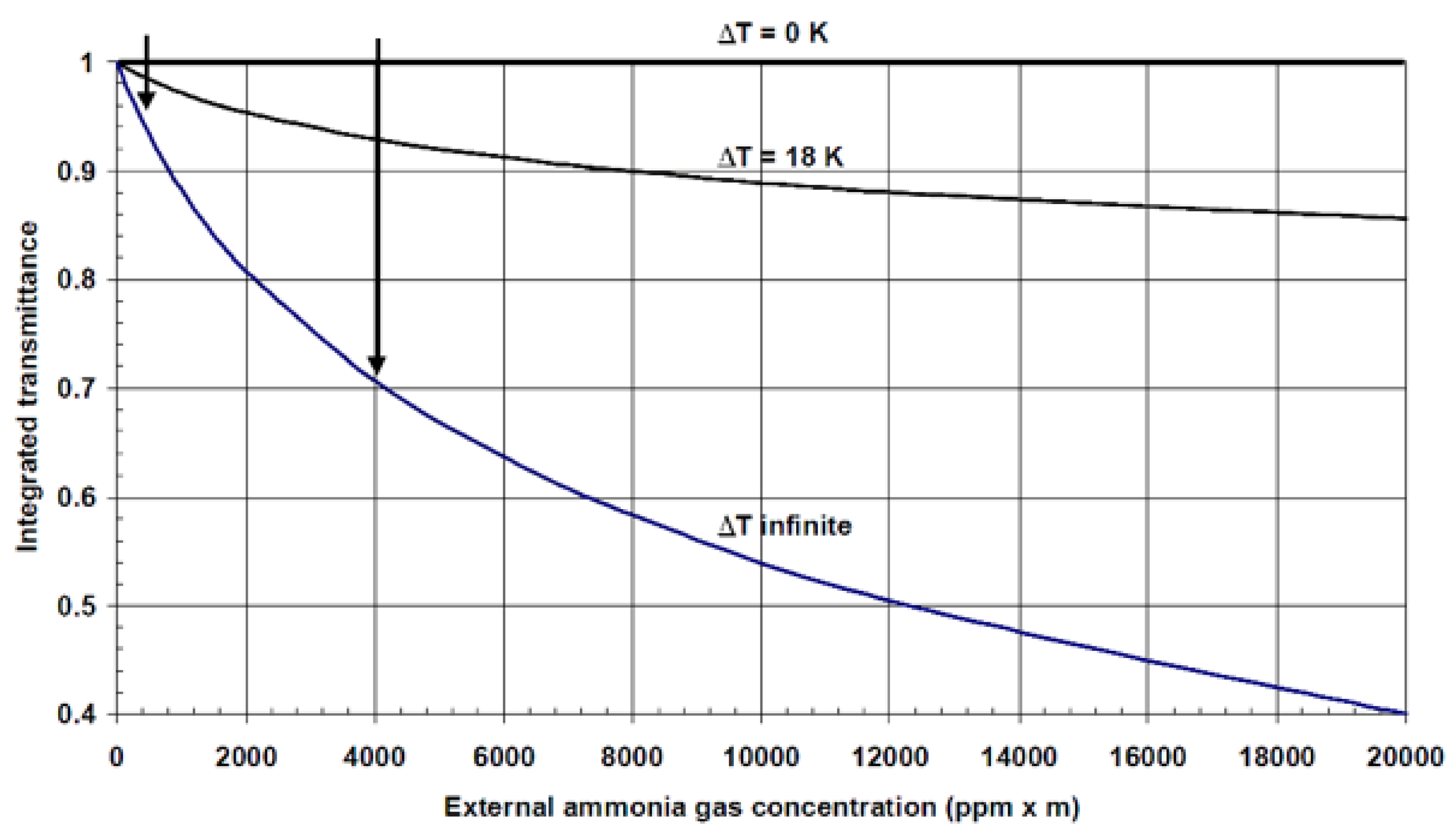
| Sandsten et al. [43,44] | Ammonia | Temperature contrast; Effective transmittance | No need to control both temperatures of background and gas cloud | Temperature information (temperature difference) is still needed |
| Wu et al. [42] | Carbon monoxide | Relative differential pixel value | Column density can be obtained without knowing temperature | Narrow, temperature-insensitive interval for specific species impedes the generalization of the method. |
| Method | Inverse Modeling Process | Advantages | Constraints |
|---|---|---|---|
| Maximum likelihood estimation | Determine the spectrum control parameter vector (temperature and column density) that results to the largest posterior probability | Statistical assessment, such as confidence | Need to construct reasonable formulas to represent probability; this is an iterative process and potentially time-consuming; initial values, learning rate, etc. need to be set manually |
| Least-squares regression | Formulate a linear explicit model of spectrum control parameter vectors , so that can be directly retrieved by linear fitting | One-step process, easy to converge | Because of the nonlinear intrinsic properties between spectrum control parameters and spectrum, the design of a linear explicit model may require considerable development and expertise |
| Levenberg–Marquardt optimization | Construct a loss function to represent the difference between synthetic spectrum and experimental spectrum, minimize the loss function by updating the spectrum control parameter vectors | It is straightforward enough to be applied to all kinds of models so long as a loss function can be constructed | Also, an iterative approach, and potentially time-consuming; initial values, weights of the various terms of the loss function, learning rate, etc. need to be set manually |
| Author | Methodology | Input | Target |
|---|---|---|---|
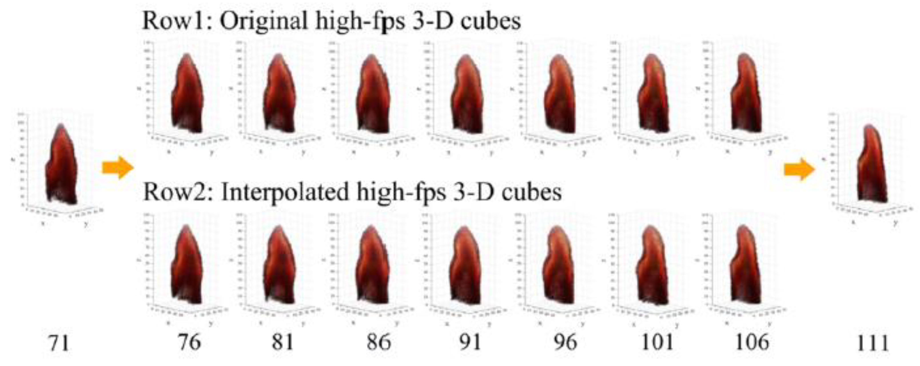
| Cai et al. [112] | CNN+ Super SloMo | 2D low FPS visual video | 3D kHz visual video of flames |
| Huang et al. [113,114] | CNN | Visual image | 3D flame structure |
| Deng et al. [115] | DBN RNN | Nonlinear Tomographic Absorption spectroscopy | Section distribution of temperature and mole concentration |
| Huang et al. [116,117] | CNN | Nonlinear Tomographic Absorption spectroscopy | Section distribution of temperature |
| Huang et al. [118] | CNN+RNN | Visual image | Prediction of flame 3D structure |
| Wei et al. [119] | CNN | Pixel layers of infrared laser absorption image | Section distribution of Methane |
| Authors | Input Format | Feature Extraction | Methodology | Target |
|---|---|---|---|---|
| Chen et al. [124] | Flame visual images | PCA | GPR | O2 concentration |
| Li et al. [125] | Flame radical images | Non-negative matrix factorization and texture analysis | Fast sparse regression | NOx concentration |
| Li et al. [126] | Flame radical images | Zernike moments | RBFN SVR | NOx concentration |
| Liu et al. [127] | Flame visual images | DBN | SVR | O2 concentration |
| Ögren et al. [128] | Flame visual images | Statistical features | GPR, MLP | H2, CO, CO2 and CH4 concentration |
| Golgiyaz et al. [129] | Flame visual images | Statistical features | MLP | Temperature, SO2, O2, NOx, CO2 and CO concentration |
| González-Espinosa et al. [130] | Flame radical images | Mean | MLP | NOx concentration |
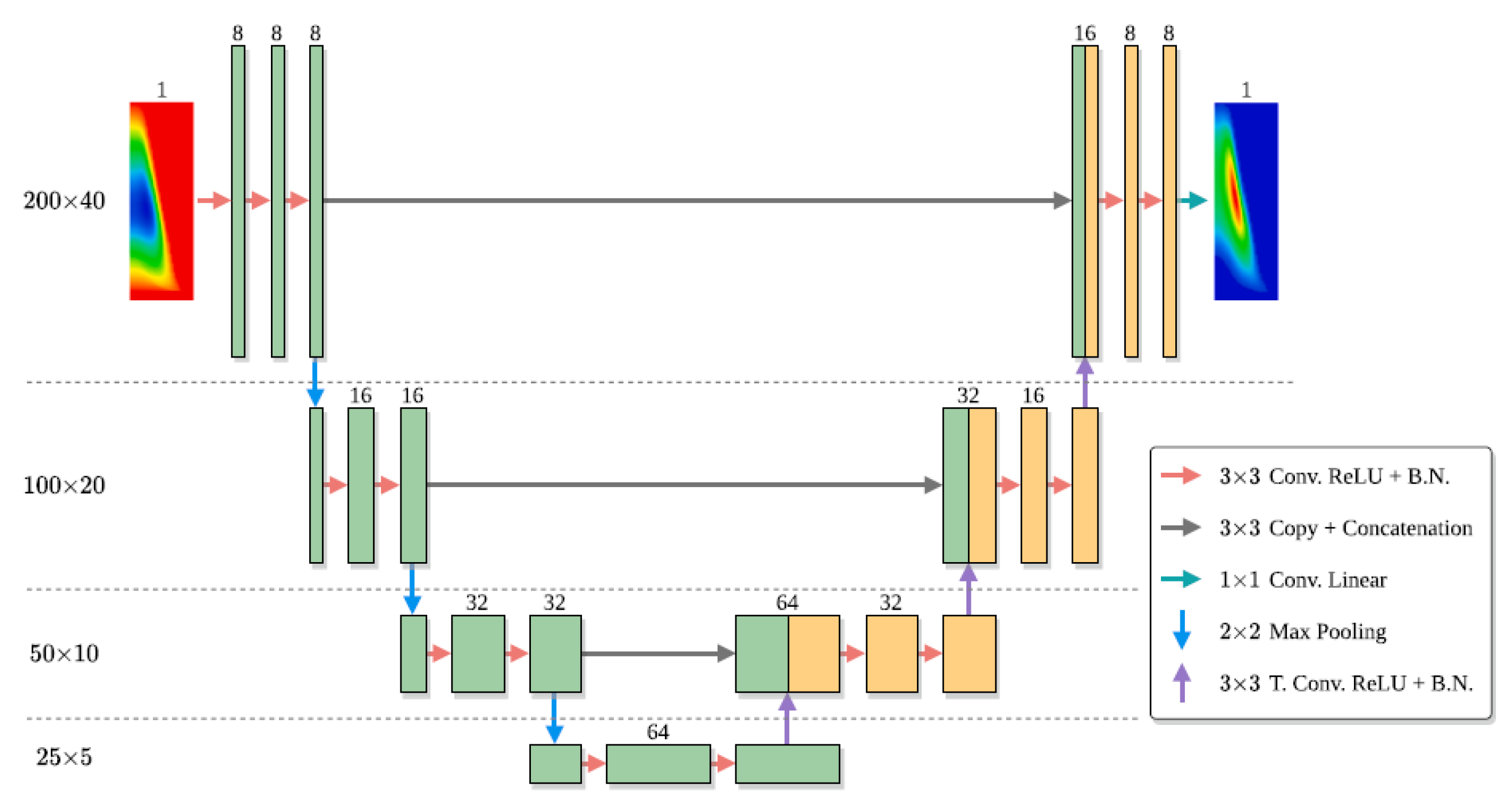
| Rodríguez et al. [123] | Flame visual images (simulated) | - | U-Net | Soot 2D concentration distribution |
Publisher’s Note: MDPI stays neutral with regard to jurisdictional claims in published maps and institutional affiliations. |
© 2022 by the authors. Licensee MDPI, Basel, Switzerland. This article is an open access article distributed under the terms and conditions of the Creative Commons Attribution (CC BY) license (https://creativecommons.org/licenses/by/4.0/).
Share and Cite
Kang, R.; Liatsis, P.; Kyritsis, D.C. Emission Quantification via Passive Infrared Optical Gas Imaging: A Review. Energies 2022, 15, 3304. https://doi.org/10.3390/en15093304
Kang R, Liatsis P, Kyritsis DC. Emission Quantification via Passive Infrared Optical Gas Imaging: A Review. Energies. 2022; 15(9):3304. https://doi.org/10.3390/en15093304
Chicago/Turabian StyleKang, Ruiyuan, Panos Liatsis, and Dimitrios C. Kyritsis. 2022. "Emission Quantification via Passive Infrared Optical Gas Imaging: A Review" Energies 15, no. 9: 3304. https://doi.org/10.3390/en15093304
APA StyleKang, R., Liatsis, P., & Kyritsis, D. C. (2022). Emission Quantification via Passive Infrared Optical Gas Imaging: A Review. Energies, 15(9), 3304. https://doi.org/10.3390/en15093304