Numerical Investigation into a New Method of Non-Axisymmetric End Wall Contouring for Axial Compressors

Abstract

To deal with corner separation in high-load axial compressors, this paper proposes a new end wall contouring method aimed at controlling the end wall secondary flow in more than one local area, generating a geometry with fewer control variables that is applicable for multiple working conditions. The new method defines more than one surface unit function, with different effects on end wall secondary flow. Then, the geometry of these surface unit functions will be superposed to generate the end wall contouring, to combine their flow control effects. After applying the new method to a bi-objective optimization design process, with 15 design variables aimed at minimizing the loss of cascade at 0° and 4° incidence, the optimal design reduces the total pressure loss of the high-load cascade by 5% under the former incidence and by 3% under the latter. The most effective design rule is constructing an end wall surface with the rising suction side and sinking pressure side in the blade channel, while locally raising the SS corner with a gentle upstream slope. According to the analysis, the design variables of the new method show an intuitive influence on the variation of end wall geometry and the movement of secondary flow. The corner separation has been effectively suppressed, with fewer control variables than before. It, thus, indicates the advantage of the newly developed end wall contouring method compared with previous studies.

1. Introduction

Since the 1940s, the total pressure ratio of the aero-engine has increased by nearly 20 times, while the stage efficiency has increased by about 10% to improve the engine’s thrust-to-weight ratio and economic efficiency [1]. Nowadays, the design of axial flow compressors is continually developed to reduce the number of stages and increase the stage pressure ratio and efficiency. This increases the stage loading of compressors, and the three-dimensional flow in the end wall region tends to be enhanced by a large inverse pressure gradient. As a result, the secondary flow and corner separation become more severe than ever, causing passage blockage, reducing the compressor’s efficiency, and even challenging the stall margin [2,3,4,5,6]. Therefore, research on end wall flow control techniques to improve the compressors’ performance has been of great interest.

As a passive flow control technique, non-axisymmetric end wall contouring (NEWC) was first proposed by Rose [7] in 1994 and was used to reduce the total pressure loss in a turbine. Brennan et al. [8] designed NEWC for a high-pressure turbine stage in a Trent 500, reducing the turbine’s secondary flow loss by 0.24% while enhancing the stage efficiency by 0.4%. As numerous numerical and experimental studies have confirmed, the basic principle of NEWC should be the variation of end wall pressure gradient due to the concave/convex end wall surface. According to the Bernoulli equation, a convex surface would form a convergent channel locally and depressurize the flow, while a concave surface has the opposite effect. Therefore, in the application of turbines, NEWC should generally weaken the boundary layer’s secondary flow, thus suppressing the corner separation and reducing the flow loss in the end wall flow field.

When applied in compressors, the design method of NEWC broadly comprises two categories in the published study. One is the empirical method. The design process uses the analytical formula or manual adjustment to create the geometry of the end wall, thereby controlling the overall intensity of the cross-passage secondary flow. Hu [9] has used the sine function in the transverse direction and generated a downslope from the pressure side (PS) to the suction side (SS), with a cubic cosine function in the axial direction to control the amplitude. This contouring suppresses the end wall secondary flow and increases the peak efficiency by 0.45%. Harvey [10] reduced the total pressure losses of a blade row by 7% with a concave center and raised the SS on the end wall surface, accelerating the secondary flow in the axial direction at the rear of the passage. A recent study by Meng et al. [11] constructed a straight downslope from the SS to the PS in an axial compressor cascade. The NEWC is combined with fillet-like corner profiling to improve the latter’s performance. The results show a reduced end wall secondary flow, and the corner separation is further suppressed. Another method by which to design NEWC is the optimization method. Compared with the empirical method, the optimization method is more commonly used. This is because the design process of the latter relies on an optimization algorithm instead of experience so that the end wall surface can be parameterized with more variables, enabling more flexible and effective control of the secondary flow. Harvey et al. [12] applied an optimization design for the NEWC on a six-stage high-pressure compressor, where the optimal NEWC created a concave surface at the front region near the SS, with a convex surface at its rear part. The NEWC facilitated the movement of the horseshoe vortex branches of the suction surface to a higher span and reduced the end wall losses by approximately 4%. Reising [13,14] conducted an optimization design process of NEWC for the compressor stage but obtained different results in the rotor and stator. The optimal end wall contouring in the stator creates a depression region near the PS, a raised region in the middle of the blade channel, and a slight drop of the end wall surface near the SS. The combined effect accelerates the secondary flow in the rear region and suppresses the development of corner separation. The end wall contouring in the rotor has a similar shape but relieves the corner separation by reducing the circumferential pressure gradient and suppressing the cross-passage secondary flow. Lepot [15] combined the blade with the NEWC. In the optimization design for the blade and then the NEWC, the latter relieves the corner separation by enhancing the cross-passage secondary flow. However, when applying a simultaneous optimization design for both the blade and the NEWC, the optimal end wall contouring improves the performance by suppressing the cross-passage secondary flow. In Dorfner’s study [16,17], the optimization design process of the NEWC automatically constructed a groove-like structure in the front passage of the compressor cascade, called an “aerodynamic separator.” This structure improves the design by creating a vortex and deflecting the cross-passage secondary flow away from the solid wall before traveling to the SS corner. A similar structure was also obtained in a subsequent investigation by Reutter [18]. In Varpe’s research [19], the NEWC parameterization used more variables for a higher degree of freedom. With nearly 100 control variables, the optimization process finally resulted in an end wall surface with complex bumps and depressions, forming a nominal upslope from the SS to the PS in the middle part of the blade channel. Li’s studies on NEWC [20,21,22] explored the flow control rules under different inflow conditions. The optimization design found that the optimal flow control rules vary with the development of corner separation and correlate with the incidence, boundary layer thickness, and boundary layer skewness of the inflow.

The above investigations reveal that the control of corner separation should require flow control force from more than one position at the end wall surface. Furthermore, the flow control rules could change with the inflow condition. Therefore, the optimization method seems more reliable than the empirical method for improving the compressor’s performance. However, the optimization method also has problems during application. Besides being time-consuming during the design iterations, the flow control rules of a particular optimal end wall contouring are usually not widely applicable. For this reason, the design rules of the end wall contouring are difficult to establish. To cope with the above problems, this study has developed a new empirical method to design the NEWC for compressors, which has been improved in the following aspects compared to the previous design method:

• The number of controlling parameters is limited to an appropriate level, making the method easy to use. The parameters have a clear and intuitive influence on the end wall geometry and the intent of flow control.
• The design space is large enough to accommodate suitable aerodynamic end wall shapes for a wide range of compressor scenarios.
• The new method can take into account the need for control of multiple local secondary flows for corner separation while facilitating the integration of prior experience of effective flow control.

2. Parametric Design of Non-Axisymmetric End Wall Contouring

To control the secondary flow in multiple local areas, the parametric NEWC generates multiple surface “units” with particular effects on the secondary flow. Then, we apply a weighted superposition to these units, as shown in Figure 1, to obtain a comprehensive flow control effect. The parametric equation for NEWC can be written as:

$$\Delta r(z,\theta )={\displaystyle \sum _{i=1}^n{w}_i{U}_i(z,\theta )}$$

(1)

where each w_iU_i(z, θ) term is a smooth and continuous function defined on the end wall z-θ plane. U_i(z, θ) refers to the variation of the radial coordinate caused by an individual end wall contouring unit, so here, we have named it the unit function for brevity; w_i is the corresponding weight factor. The overall shape of the NEWC will, thus, be dependent on each unit function and weight factor. Considering the previous research outlined in the Introduction, the new method proposes two types of unit functions.

2.1. The Definition of the End Wall Contouring Units

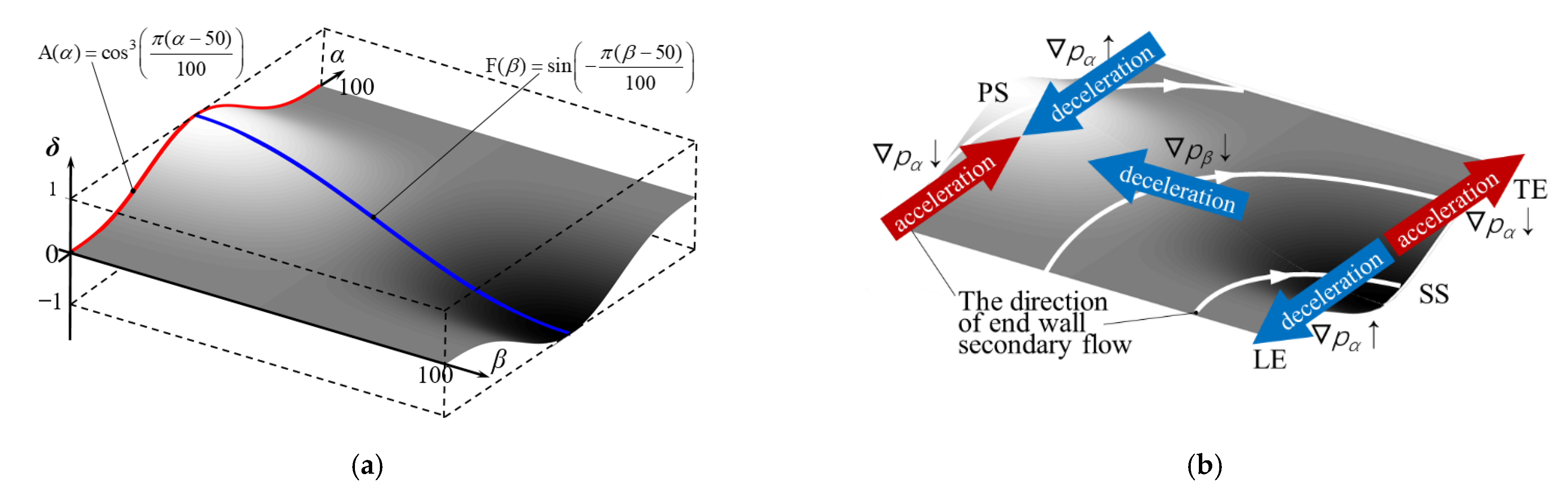
2.1.1. The Continuous Unit

The first type of NEWC unit is designed to accelerate or decelerate the full-area cross-passage secondary flow. We have named it the “continuous unit” for brevity. The design is shown in Figure 2. For the convenience of presentation, Figure 2a maps the z-θ end wall surface of the blade channel to a standard space of {(α, β, δ)| α∈[0, 100], β∈[0, 100], δ∈[−1, 1]}. Here, α, β, and δ represent the streamwise, circumferential, and radial directions of the blade channel, respectively, while u_i represents the unit function in the standard space, corresponding to U_i in Equation (1). α = 0 and α = 100 represent the leading edge (LE) and trailing edge (TE) lines, respectively; β = 0 and β = 100 represent the PS and SS, respectively. Then, the control equations of the continuous unit can be expressed as:

$$u_i=w_i\mathrm{F}(\beta )\mathrm{A}(\alpha )=w_i\sin \left(-\frac{\pi (\beta -50)}{100}\right){\cos }^3\left(\frac{\pi (\alpha -50)}{100}\right).$$

(2)

Equation (2) shows that the continuous unit has only one control variable, i.e., w_i. The streamwise function, i.e., A(α) = cos³(π(α − 50)/100), acts as the amplitude of the circumferential function F(β) = sin(−π(β − 50)/100), and the maximum value of A(α) is located at α = 0.5. When the continuous unit is mapped to the actual end wall of the axial flow compressor, the shape of the surface causes the suction side of the blade channel to sink and the pressure side to rise, with the maximum slope in the 0.5 axial chord length (C_a) position. Thus, Figure 2b illustrates the possible variation of end wall flow, according to the Bernoulli effect. The continuous unit generates an upslope surface from the SS to the PS in the circumferential direction, as reported in previous studies [9,11]. Therefore, the circumferential pressure gradient (ᐁP_β) decreases and the cross-passage secondary flow decelerates in the entire area. Besides these events, there are also some side effects. On the suction side of the end wall, the variation of the streamwise pressure gradient (ᐁP_α) will keep positive from the LE to the mid-chord and then is negative until TE. Therefore, the streamwise component of end wall flow will decelerate in the front half and accelerate in the rear half. On the pressure side of the end wall, all side effects are on this opposite side of those on the suction side. It should also be noted that when applied to an actual compressor, all the above flow control, including its impact on the cross-passage secondary flow and the side effects, may turn in the opposite direction when w_i is less than zero.

2.1.2. The Localized Unit

The second type of end wall contouring unit is defined as a design to facilitate localized secondary flow control in the blade channel. Therefore, it is named the “localized unit” for brevity. The design of this end wall contouring unit is shown in Figure 3a.

The streamwise configuration corresponds to the side-view in the dashed red box. Different from the continuous unit, the control equation of the localized unit is defined by four control variables, i.e., { κ_s, κ₁, κ₂, κ₃}. The equation is:

$$A(\alpha )=\left\{\begin{array}{l}0, \alpha <{\alpha }_1\\ \mathrm{cspline}(({\alpha }_1,0),({\alpha }_2,1)), {\alpha }_1<\alpha <{\alpha }_2\\ 1, {\alpha }_2<\alpha <{\alpha }_3\\ \mathrm{cspline}(({\alpha }_3,1),({\alpha }_4,0)), {\alpha }_3<\alpha <{\alpha }_4\\ 0, {\alpha }_4<\alpha <1\end{array}\right.$$

(3)

where:

$$\left\{\begin{array}{l}{\alpha }_2=100{\kappa }_s, 0.1\le {\kappa }_s\le 0.9\\ {\alpha }_3={\alpha }_2+100\left(0.9-{\kappa }_s\right){\kappa }_1, 0\le {\kappa }_1\le 1\\ {\alpha }_1={\alpha }_2-\left(10+100\left({\kappa }_s-0.1\right){\kappa }_2\right), 0\le {\kappa }_2\le 1\\ {\alpha }_4={\alpha }_3+\left(10+\left(90-{\alpha }_3\right){\kappa }_3\right), 0\le {\kappa }_3\le 1\end{array}\right.$$

(4)

In the above equations, κ_s and κ₁ are the starting factor and ending factor of the streamwise configuration, respectively, which determine the axial range of the convex profile, i.e., (α₂, 1) and (α₃, 1). κ₂ and κ₃ are intended to adjust the slope at the starting and ending sections, to calculate (α₁, 0) and (α₄, 0). After determining the four control points, the control equations of the upslope section (α₁ < α < α₂) and the downslope section (α₃ < α < α₄) are constructed, respectively, by using the cubic spline interpolation function with boundary conditions to keep the slope of the boundary at 0, thus ensuring a smooth connection between the shaped section and the unshaped part.

The circumferential configuration is shown from the front view in the dashed blue box in Figure 3a. The control equation is defined by:

$$\mathrm{F}(\beta )=\left\{\begin{array}{l}-1, \beta <{\beta }_1\\ \sin \left(\frac{\pi }{{\beta }_2-{\beta }_1}\left(\beta -\frac{{\beta }_1+{\beta }_2}{2}\right)\right), {\beta }_1\le \beta \le {\beta }_2\\ 1, \beta >{\beta }_2\end{array}\right.$$

(5)

where:

$$\left\{\begin{array}{l}{\beta }_1=100{\kappa }_l, -1\le {\kappa }_l\le 0.9\\ {\beta }_2=100{\kappa }_r, {\kappa }_l\le {\kappa }_r \mathrm{and} 0.5\le {\kappa }_r\le 2.0\end{array}\right.$$

(6)

It is obvious that F(β) is defined by κ_l, κ_r and bends upward on the end face between β ∈ [β₁, β₂], forming an “upslope”. According to the previous research mentioned in the Introduction, this configuration will enhance the circumferential pressure gradient within β ∈ [β₁, β₂] and enhance the end wall secondary flow.

Using the streamwise and circumferential equation, the control equation of the localized unit can be written as:

$$u_i=w_i\mathrm{A}(\alpha )(\mathrm{F}(\beta )+k_0)$$

(7)

where k₀ is the zeroing factor to keep a constant cross-sectional area of the blade channel. It is defined by:

$${\displaystyle {\int }_0^{100}\mathrm{F}(\beta )=0}$$

(8)

Figure 3b shows the possible variation of the pressure field and the end wall secondary flow when applying a localized unit. If w_i > 0, the end wall surface would form an upslope surface from β₁ to β₂. Therefore, the circumferential pressure gradient within {(α, β) | β∈[β₁, β₂] ∩ α∈[α₁, α₄]} will increase, thus accelerating the cross-passage secondary flow locally. The side effects are similar to the continuous unit. On the suction side of the profiling region, the variation of ᐁP_α will accelerate the streamwise end wall flow within α∈[α₁, α₂] and decelerate it within α∈[α₃, α₄]. On the pressure side, the side effects manifest the opposite way round. In addition, all the flow control may turn in the opposite direction when w_i < 0.

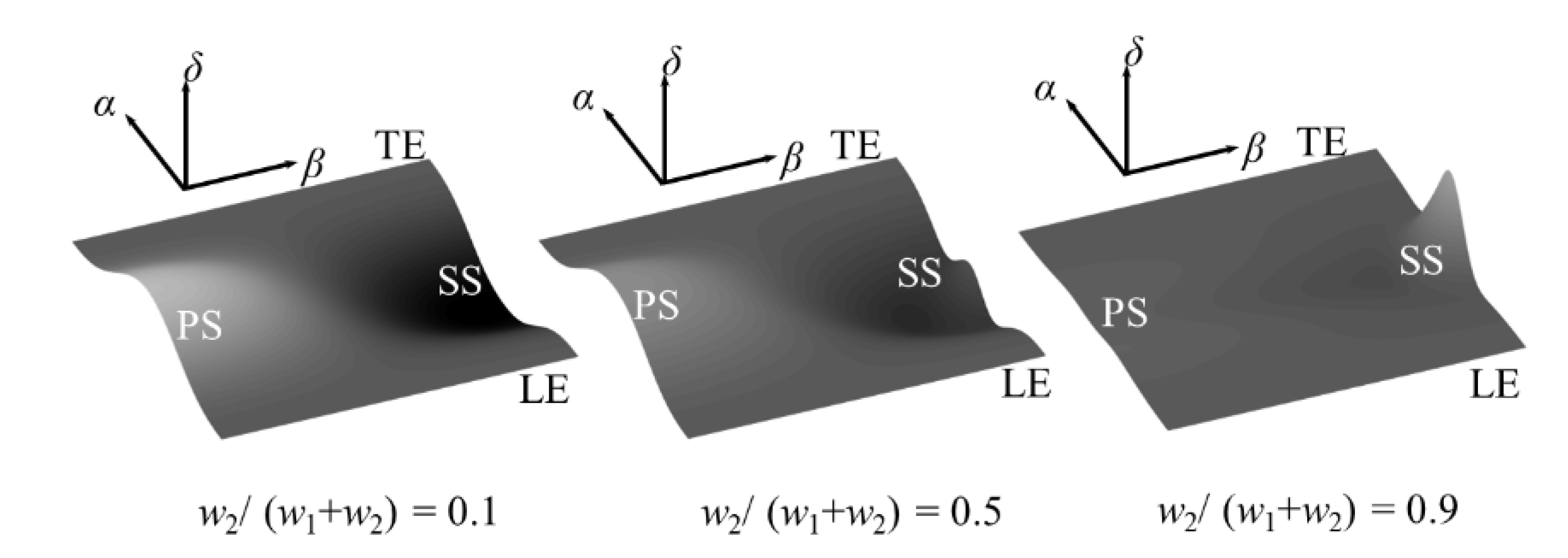
2.2. Generating Non-Axisymmetric End Wall Contouring in the Standard Space

In the next step, the above two types of end wall contouring units, as defined in Equations (2) and (7), are combined in the standard space. Note that each of the units has the effect of enhancing or weakening the end wall secondary flow in a particular region. Thus, the physical result of combining them is to superimpose their effects in flow control, finally obtaining an end wall surface with comprehensive effects. Therefore, supposing there are n units (labeled as u₁ to u_n) included in an NWEC, the combination would be:

$$H=w_1{u}_1+w_2{u}_2+w_3{u}_3\dots +w_n{u}_n$$

(9)

The weight factor w_i represents the emphasis on different flow control effects.

Figure 4 illustrates the variation of the end wall surface by adjusting the weight factors. For an end wall surface consisting of a continuous unit and a localized unit, the former is designed to suppress the cross trend of the full-area end wall secondary flow, while the latter is intended to accelerate secondary flow in the SS corner region. Their weight factors are defined as w₁ and w₂, respectively. When w₂/(w₁ + w₂) changes from 0.1 to 0.9, the overall slope of the surface from SS to PS gradually weakens, and the local shape along the SS corner becomes more and more prominent.

Strictly speaking, the linear combination of the geometry does not equal a linear combination of their flow control effects. However, the characteristics of the NEWC surface show that the effect of the localized unit on the end wall flow near the SS corner gradually increases with w₂/(w₁ + w₂).

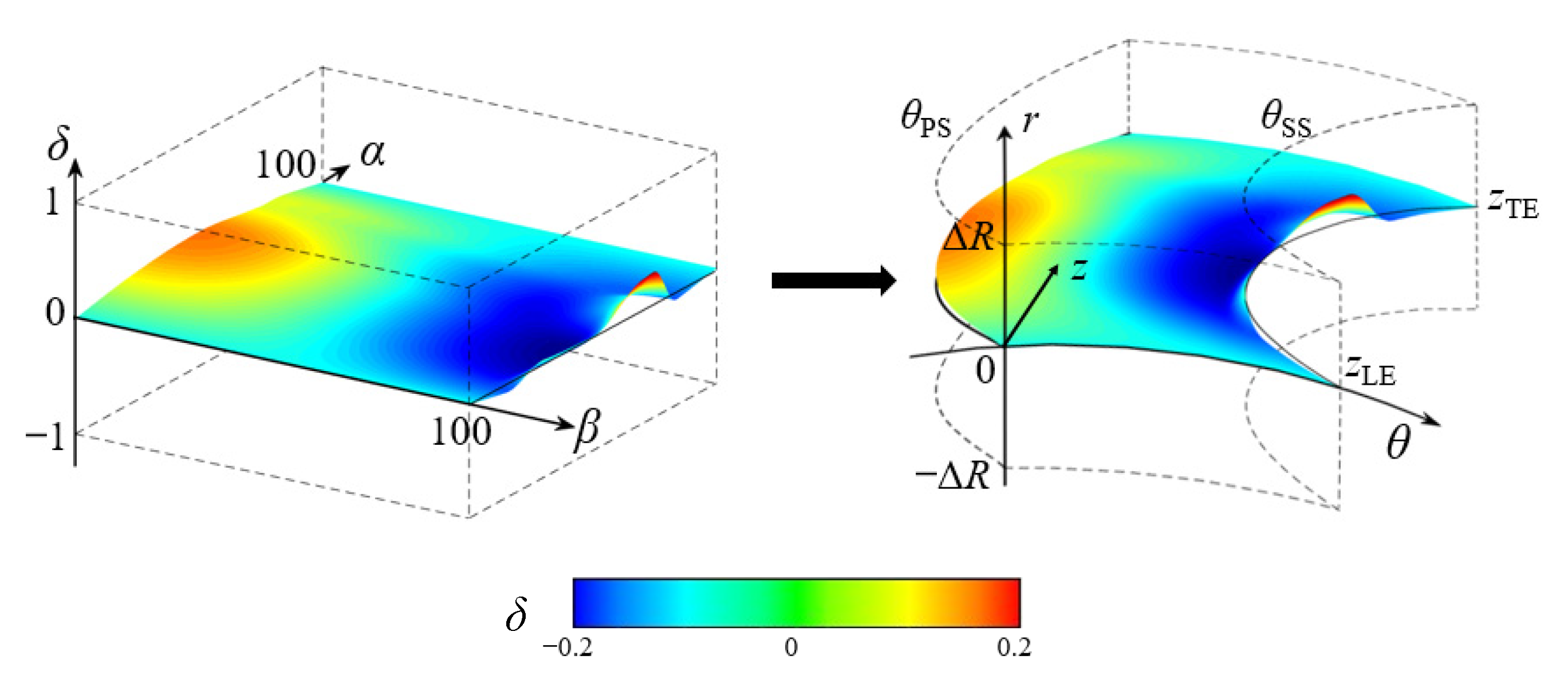
2.3. Generating NEWC for the Actual Compressor

After obtaining the end wall contouring in the standard space of {(α, β, δ)| α∈[0, 100], β∈[0, 100], δ∈[−1, 1]}, the surface of the end wall contouring can be mapped directly to the three-dimensional end wall region of the axial compressor, according to their spatial correspondence. Figure 5 shows an example of this. The coordinate system of the compressor end wall region is (r, θ, z). r₀ represents the radius of the baseline end wall surface; z_LE and z_TE represent the LE and TE axial coordinates; θ_PS and θ_SS represent the circumferential coordinates of the PS and the SS. Here, the z_LE, z_TE, θ_PS and θ_SS correspond to α = 0, α = 100, β = 0 and β = 100, respectively. Furthermore, if limiting the waviness of the actual end wall contouring within ±ΔR, the NEWC in the standard space can be mapped to its actual geometry in the axial compressor through the equation:

$$\left\{\begin{array}{l}r=\Delta r+r_0(z)=\delta \Delta R(z)+r_0(z)\\ z=\alpha (z_{TE}-z_{\mathrm{LE}})/100+z_{\mathrm{LE}}\\ \theta =\beta ({\theta }_{\mathrm{SS}}(z,r)-{\theta }_{\mathrm{PS}}(z,r))/100+{\theta }_{\mathrm{PS}}(z,r)\end{array}\right.$$

(10)

The above section discusses the definition and implementation process of this new end wall contouring method. Note that the new method can theoretically create arbitrary shapes by combining an infinite number of end wall contouring units. However, our experiences during application suggest that combining one continuous unit and two localized units will usually be sufficient to control the corner separation. Therefore, the new method generally requires 8 to 15 parameters for all the design processes.

3. The Baseline Compressor Cascade and CFD Method

In this study, a high-load linear compressor cascade was chosen to verify the effectiveness of the new end wall contouring method. Using a linear cascade instead of an actual compressor can keep the investigation from the influence of twisted blade sections, leakage flow, centrifugal force, and inlet boundary layer skew. Thus, only the most common features of a high-load compressor, i.e., the inlet boundary layer and the secondary flow, were considered and the results will be universal. Note that in the Cartesian coordinate of the linear cascade, the directions of z, y, and x are equivalent to z, θ, and r, as defined in the end wall contouring method.

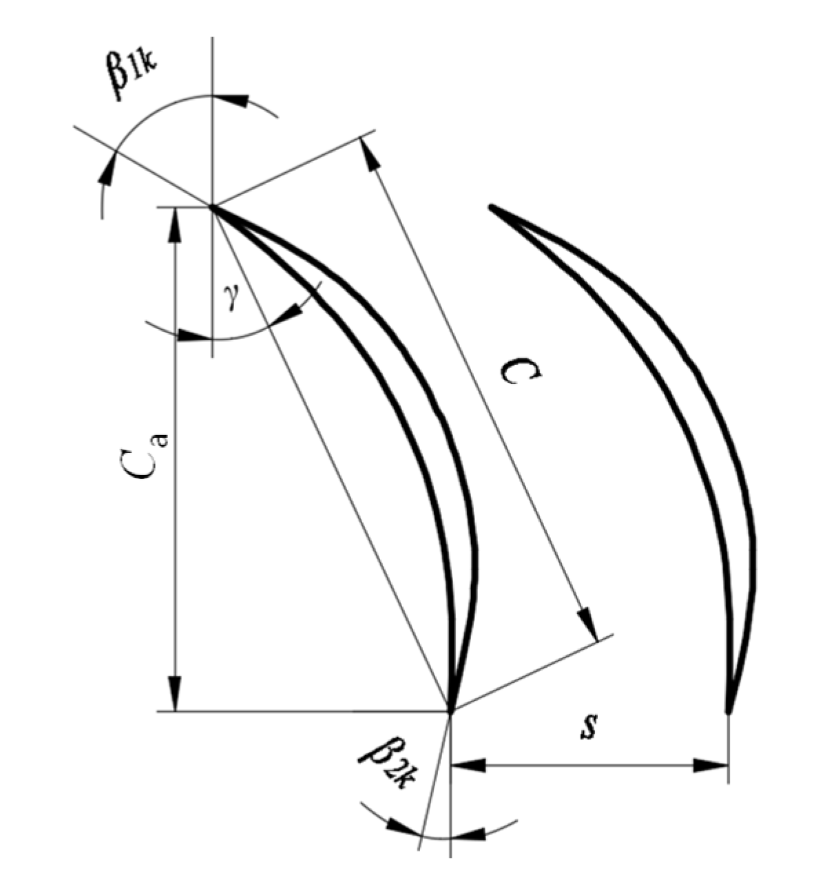
3.1. The Baseline Compressor Cascade and the Experimental Test Rig

The geometry of the baseline cascade comes from the hub region of a stator blade in the rear stage of a high-load compressor. The camber angle is more than 55°, with a solidity (s) larger than 2.0 and a designed axial outflow. After rounding off the geometry and inflow conditions, the parameters of the cascade are shown in Figure 6 and

Table 1. Design parameters of the baseline cascade.

Parameters	Values
Heigh of the blade (h)	100 mm
Chord (C)	40 mm
Axial chord (Ca)	36.2 mm
Pitch (s)	20 mm
Inlet blade angle (β1k)	59°
Outlet blade angle (β2k)	10°
Stagger angle (γ)	25°

.

The experiment was carried out in the Key Laboratory of Marine Gas Turbine Technology in Liaoning Province. The test of the baseline cascade was taken over five different incidences, with an inlet Mach number of 0.6. The compressor cascade consisted of 10 blades to ensure periodicity in the central blade channel. The inlet flow field was measured by the total pressure probe and static pressure probe at 1.2C_a upstream of the LE. A five-hole probe was located at 0.5C downstream of the TE to measure the outlet aerodynamic parameters from the end wall to the mid-span. Multiple pressure taps were placed on the end wall to capture the static pressure.

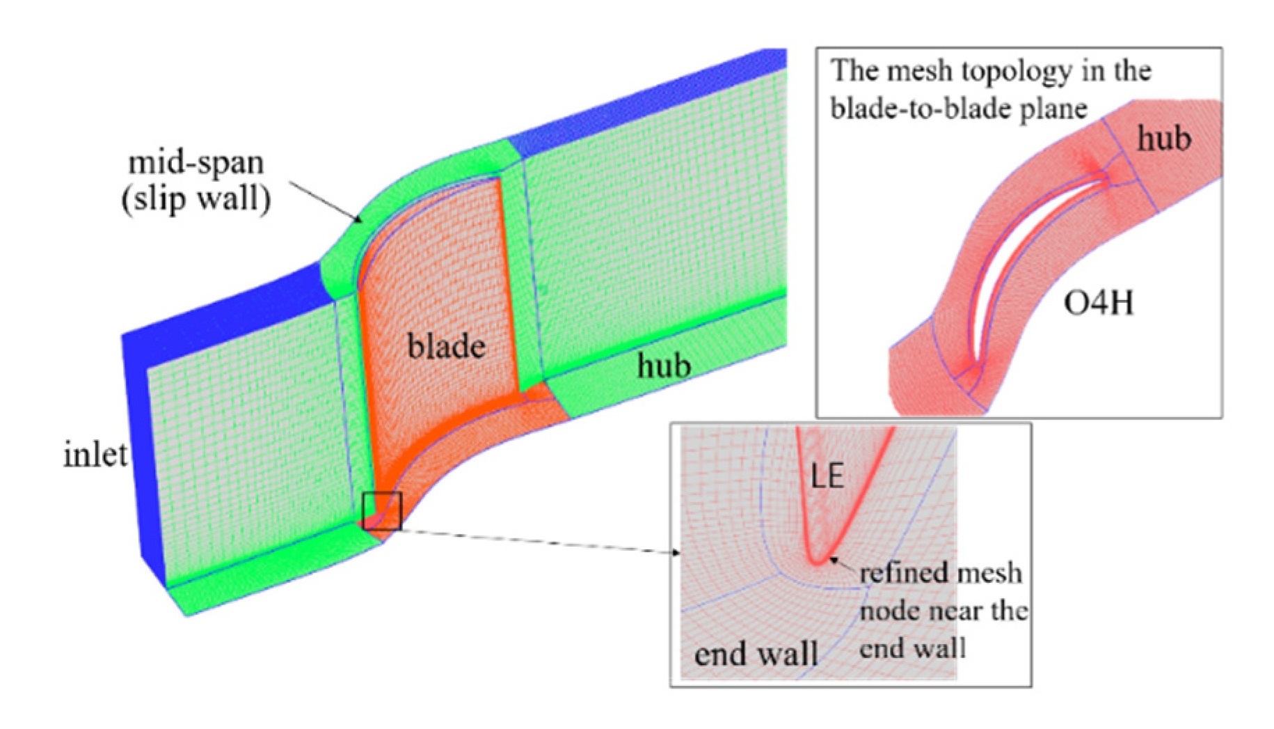
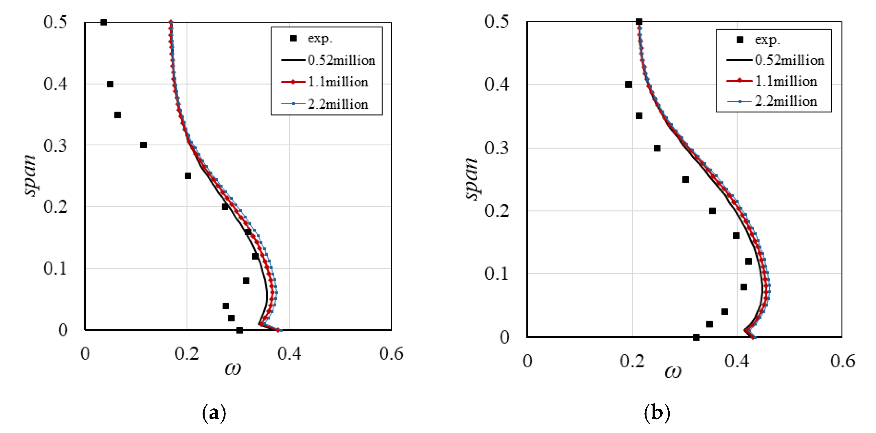
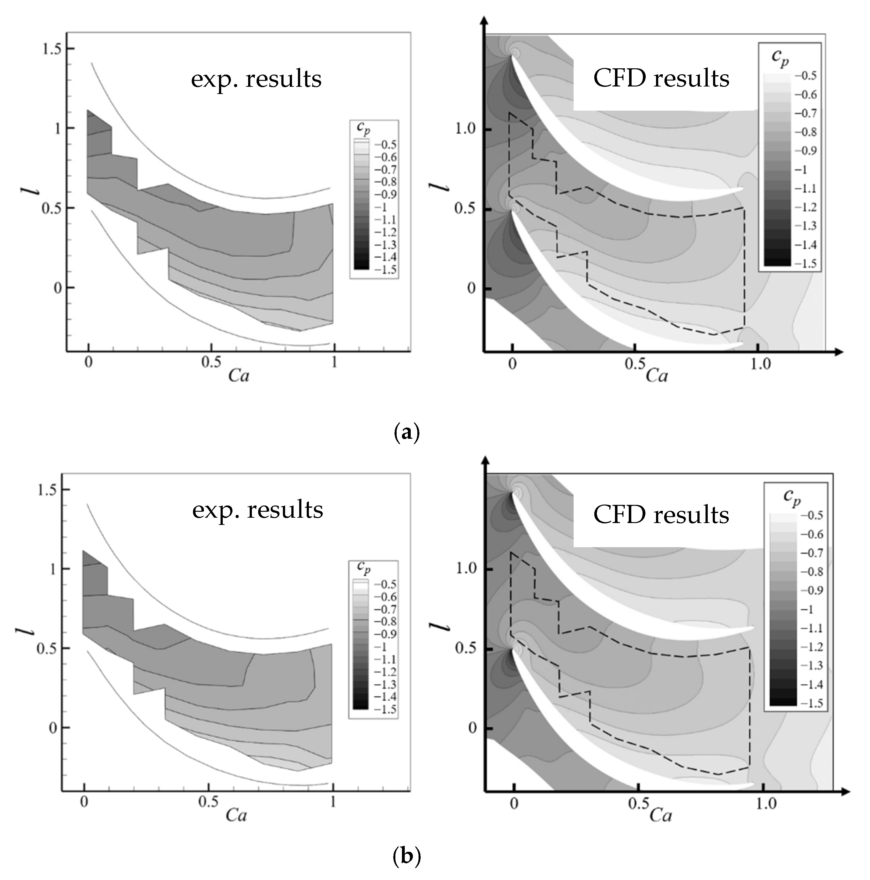
3.2. The CFD Method and Validation

A three-dimensional steady simulation was carried out for the investigation. The computational domain only included a single-passage half-span flow region of the cascade. The inlet boundary of the computation domain locates 1.2C_a upstream of the LE. The outlet boundary extends to 2.0C_a downstream of the TE to ensure sufficient mixing of the outflow. Figure 7 shows the mesh of the computational domain (with a cutaway view). The mesh is generated using IGG/Autogrid from the NUMECA package. To improve the mesh quality, H topology is used for both the inlet and outlet sections, and an “O4H” topology is used for the blade channel. The nodes of the mesh are refined near the solid wall of the blade and the hub. The average y⁺ of the first-layer mesh near the solid wall is less than 1.

The flow field of the cascade is calculated by solving the steady Reynolds-averaged Navier–Stokes (RANS) equations with ANSYS CFX, using the second-order upwind scheme. The baseline k-ω model (BSL) is selected from several turbulence models for its accuracy and convergence when calculating separation problems. The boundary conditions are given according to the experimental results. The inlet boundary condition defines the inflow velocity and the static temperature, while the outlet boundary condition defines the static pressure at sea level. In addition, the circumferential boundaries use the periodic boundary condition; the mid-span plane uses the slip-wall boundary condition. The convergence criterion is set to 1 × 10⁻⁶ for the RMS residual values.

With the above settings, a grid independence study was performed. Three groups of mesh, with 0.52 million nodes, 1.1 million nodes, and 2.2 million nodes, were generated with the same topology. Figure 8 shows their pitch averaged total pressure loss coefficients, which are defined as:

$$\omega =\frac{P_{\mathit{1}}^{*}-P^{*}}{P_{\mathit{1}}^{*}-P_{\mathit{1}}}$$

(11)

where P₁^* and P₁ represent the inlet total pressure and static pressure at the 0.5span, respectively. P^* is the pitch-wise averaged total pressure at 0.5C downstream of the TE.

According to Figure 8, the three groups of mesh show nearly the same spanwise distribution of ω at the design point (OP1, i = 0°) and with an increased incidence (OP2, i = 4°). The difference in ω due to mesh number is about 0.01 below 0.3span and almost equals 0 between 0.3span and 0.5span. A further increase in mesh number seems not to bring significant computational benefits. Considering the significant differences between the three mesh groups in computing time during the optimization design, their impact on the cascade performance seems relatively small. Therefore, to have a higher resolution of the flow field with an acceptable computing time, the mesh with 1.1 million nodes was selected for the CFD study.

Figure 8 provides the experimental results. At OP1, the calculated ω in Figure 8a approximates the experimental data below 0.2span but reaches a larger value above 0.2span. Because the former region is the core area of loss in close relationship with the corner separation, while the two-dimensional separation influences the latter part more, this indicates that the CFD method predicts the corner separation accurately but is less effective in calculating the two-dimensional separation on the SS for such a high-load compressor cascade. At OP2, when there is an increased incidence, the calculated ω in Figure 8b shows a similar trend from the loss core (below 0.2span) to the mid-span, but with a uniformly full range over prediction. Therefore, the above results indicate that the CFD method may have some shortfalls when predicting the two-dimensional separation. However, the simulation values relevant to the corner separation are generally consistent with the experimental results, whether for the loss prediction or the increase of loss due to a higher incidence.

In addition, Figure 9 gives the distribution of end wall static pressure coefficients (c_p) for the experimental and CFD results, which are defined as:

$$c_p=\frac{P-P_{\mathit{1}}^{*}}{P_{\mathit{1}}^{*}-P_{\mathit{1}}}$$

(12)

where P represents the static pressure on the end wall; P₁^* and P₁ are the same as in Equation (11). The outline of the experimental contour is added as black dashed polylines in the calculated contours for the convenience of comparison. Figure 9 shows that the calculated c_p is consistent with the experimental results under both working conditions. Considering that the development of corner separation is mainly related to the secondary flow in the end wall area, which is driven by the end wall pressure gradient, this may explain the reason for the accurately calculated loss of core area caused by the corner separation in Figure 8.

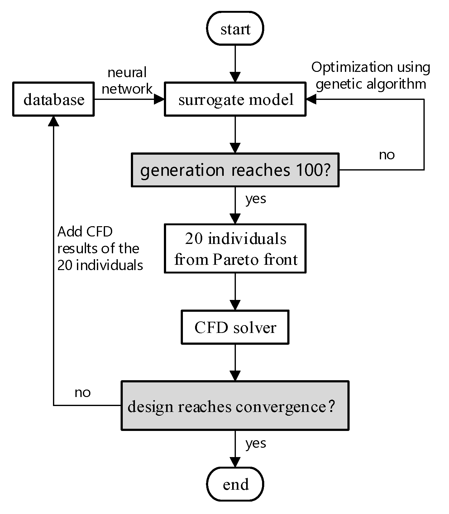
4. Optimization Method

When applying the NEWC, it is expected that the loss of the compressor can reduce pressure across the operating range. In particular, reducing the total pressure loss coefficient at both OP1 and OP2 means improving the efficiency at the design stage and near the stall condition for the compressors’ applications. Previous studies [20,23] also found that reducing total pressure loss at both OP1 and OP2 also means reducing the loss between these two operating points. Therefore, a multi-objective numerical optimization design is carried out, based on the parameterization method in Section 2, to minimize the total pressure losses at OP1 and OP2. The total pressure loss coefficient is defined as:

$${\omega }_o=\frac{P_{\mathrm{outlet}}^{*}-P_{\mathrm{inlet}}^{*}}{P_{\mathrm{inlet}}^{*}-P_{\mathrm{inlet}}}$$

(13)

where P_inlet and P*_inlet represent the mass flow averaged total pressure and static pressure at the inlet, while P*_outlet for the mass flow averaged the total pressure at the outlet.

A continuous unit and two localized units are used for parametric end wall contouring. Therefore, this includes 15 control variables in total, i.e., the amplitude of continuous unit w₁; the amplitude, axial/circumferential control variables of the first localized unit {w₂, κ_s,1, κ_1,1, κ_2,1, κ_3,1, κ_l,1, κ_r,1}; and the amplitude, axial/circumferential control variables of the second localized unit {w₃, κ_s,2, κ_1,2, κ_2,2, κ_3,2, κ_l,2, κ_r,2}. The process of optimization design is shown in Figure 10. The optimization process is controlled using the software ISIGHT, with a two-layer iteration. First, a database of 100 NEWC geometries was generated by random sampling over the 15 control variables. A simulation was carried out to establish the total pressure loss coefficients at OP₁ and OP₂ (defined as ω_o1 and ω_o2), thus obtaining a database including seven times the control variables. The inner iteration uses the database to train a radial basis neural network model, between the control variables and the loss coefficients. The neural network functions as the surrogate model for CFD calculations. The NSGA-II algorithm is applied as the optimizer. After 100 iterations based on the estimation of the neural network, a total of 20 individuals were selected as being the optimal results of the internal iteration. In the outer iteration, ω_o1 and ω_o2 of the 20 individuals were verified by CFD simulations, then the CFD results were added to the database. The next iteration thus began. The optimization process would be stopped either when it reached convergence or when the outer iteration exceeded 20 steps.

The most time-consuming part of the actual optimization process was the CFD simulation. It was accomplished on a workstation with an i7-10700k CPU (3.8 GHz). The performance of each end wall contouring required up to 300 steps of simulation for each operating point, which took about 2 h, with ten CPU threads. The actual optimization process reached convergence in 7 steps of the outer iterations and finally took about three weeks to get the final result. Note that with bi-objective optimization, a process that reaches convergence within seven steps means a much faster convergence speed than the traditional method. This is likely because there are fewer control variables in the new method, making the neural network more accurate over a particular number of samples in the database.

5. Results and Discussion

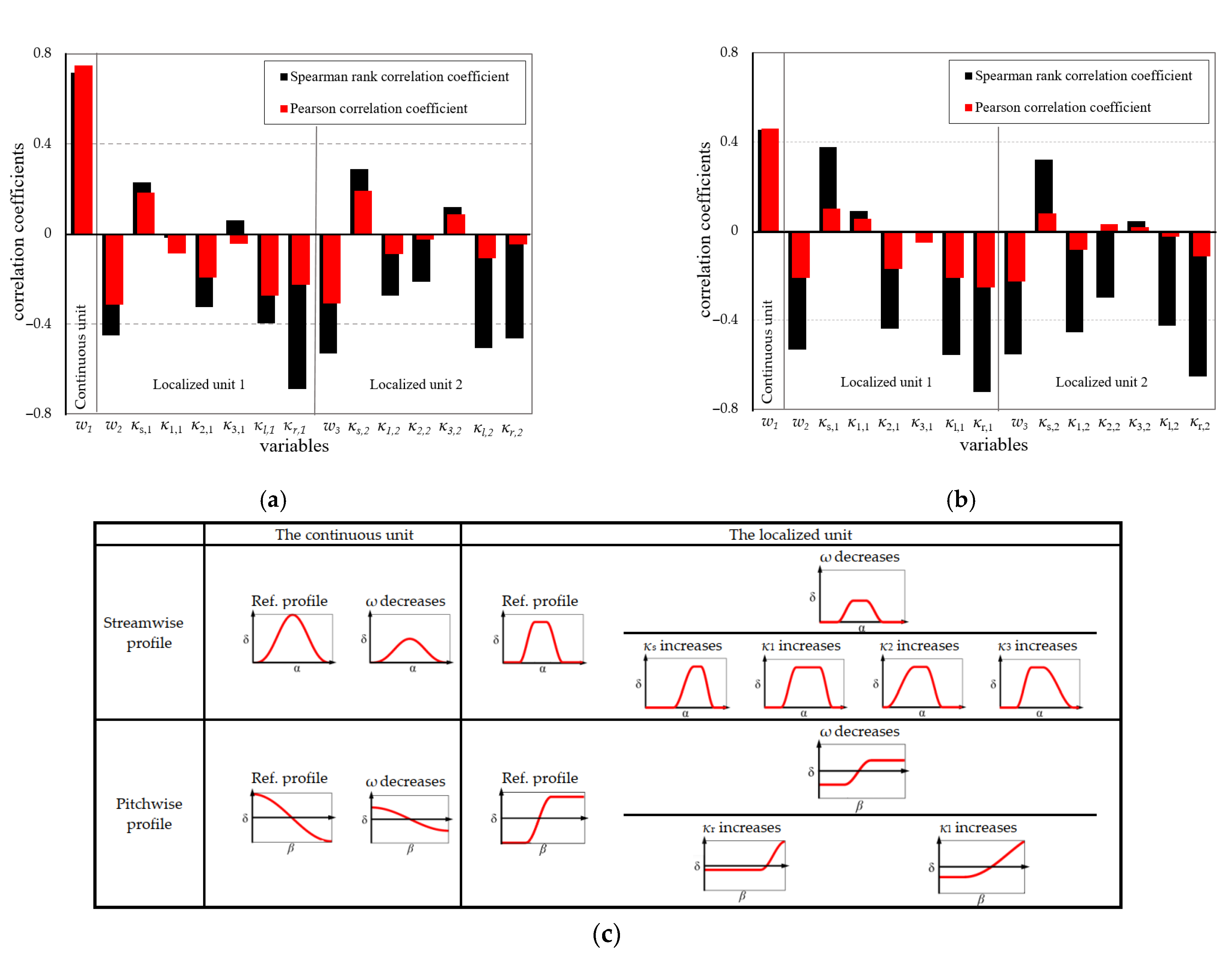
5.1. Correlation Analysis of Control Variables and Losses

Since all the control variables for NEWC were associated with the secondary flow control in the end wall region, in the first step, correlation analysis over the samples of the optimization process was carried out to establish the generally effective rules of end wall contouring. The effect of each variable on the total pressure loss was explored using the Spearman rank correlation coefficient (Γ_S). The Pearson partial correlation coefficient (Γ_P) was further used to explore the independent influence of each variable on losses.

In Figure 11, the horizontal coordinate from left to right represents the 15 design variables for the current end wall contouring, which are separated into three groups according to their surface units. A schematic plot is also added below to illustrate how the variation of design variables would affect the variation of the end wall contouring units. The vertical coordinate indicates the correlation coefficient between the total pressure loss coefficient (ω_o) and the above control variables. The black bars show the values of Γ_S, and the red bars are for Γ_P. Γ > 0 indicates that the loss positively correlates with the variables, i.e., a larger value of the variable induces a higher loss. Γ < 0 indicates the opposite. Here, we defined |Γ| ≤ 0.4 as a low correlation, 0.4 < |Γ| ≤ 0.7 as a medium correlation, and 0.7 < |Γ| ≤ 1 as a high correlation.

The Spearman rank correlation coefficient at OP2 was first analyzed. According to Figure 11a, the Γ_S between w₁ and ω_o2 is 0.71, indicating a high positive correlation. This means that a smaller amplitude of the continuous unit is much more favorable for loss control. Therefore, reducing the concave near SS and the convexity near PS, or even reversing them, i.e., enhancing the end wall secondary flow toward the SS, would bring more benefits. The Γ_S of w₂ and ω_o2 is −0.45, representing a medium negative correlation. In other words, it is more helpful to control loss when the contouring forms an upslope to SS. The values of |Γ_S| corresponding to the control variables κ_s,1, κ_1,1, κ_2,1, κ_3,1 were all less than 0.4, indicating that the axial control variables of the first localized contouring unit are less influential on loss. However, by considering the positive and negative values of Γ_S, it can still be judged that placing the unit near the LE with a slight upstream slope helped to reduce the loss of the front section; meanwhile, the position and slope of the rear section have little influence. The circumferential control variables of the first localized unit, i.e., (κ_l,1, κ_r,1), both have a medium negative correlation with w₂, so a larger κ_l,1, κ_r,1, i.e., generating the circumferential upslope near the SS would tend to reduce loss. The correlation coefficients of the second localized unit were similar to the first localized unit, except that the Γ_S between κ_2,1 and ω is about −0.4. This indicates that constructing the second localized contouring unit with its rear section near the TE was conducive to controlling loss.

Compared with Γ_S, the red bars in Figure 11a show that the Pearson partial correlation coefficients Γ_P of the localized units were notably reduced after excluding the effects of the other variables; however, they showed generally the same positive/negative signs. Therefore, on the one hand, this means that the results of Γ_P agree with the end wall contouring rules concluded from Γ_s. On the other hand, this also indicates that the effects of each variable of the localized unit on losses were strongly influenced by the other variables, i.e., there is a strong correlation among them.

As for OP1 in Figure 11b, the rules of end wall contouring shown from the data are similar to those in the above discussion at OP2. The main difference is that the correlation coefficient between w₁ and ω_o1 decreased significantly, meaning a much weaker effect of the full-area unit on the overall performance.

To summarize, the correlation analysis indicates the following:

• The correlation between the control variables of the localized units and the overall loss was nonlinear. The control variables of the localized units were found to be strongly interrelated with each other when suppressing the corner separation and reducing losses.
• The most effective end wall contouring in separation control required the continuous unit to generate a convex end wall near the SS and a concave end wall near the PS. For the localized units, a convex end wall near the SS extending to LE and TE, with a gentle slope toward the LE, tended to minimize the overall loss.
• The contouring rules under different working conditions were similar. In the operating point of high incidence, the control of corner separation was more closely associated with the localized control of secondary flow near the SS.

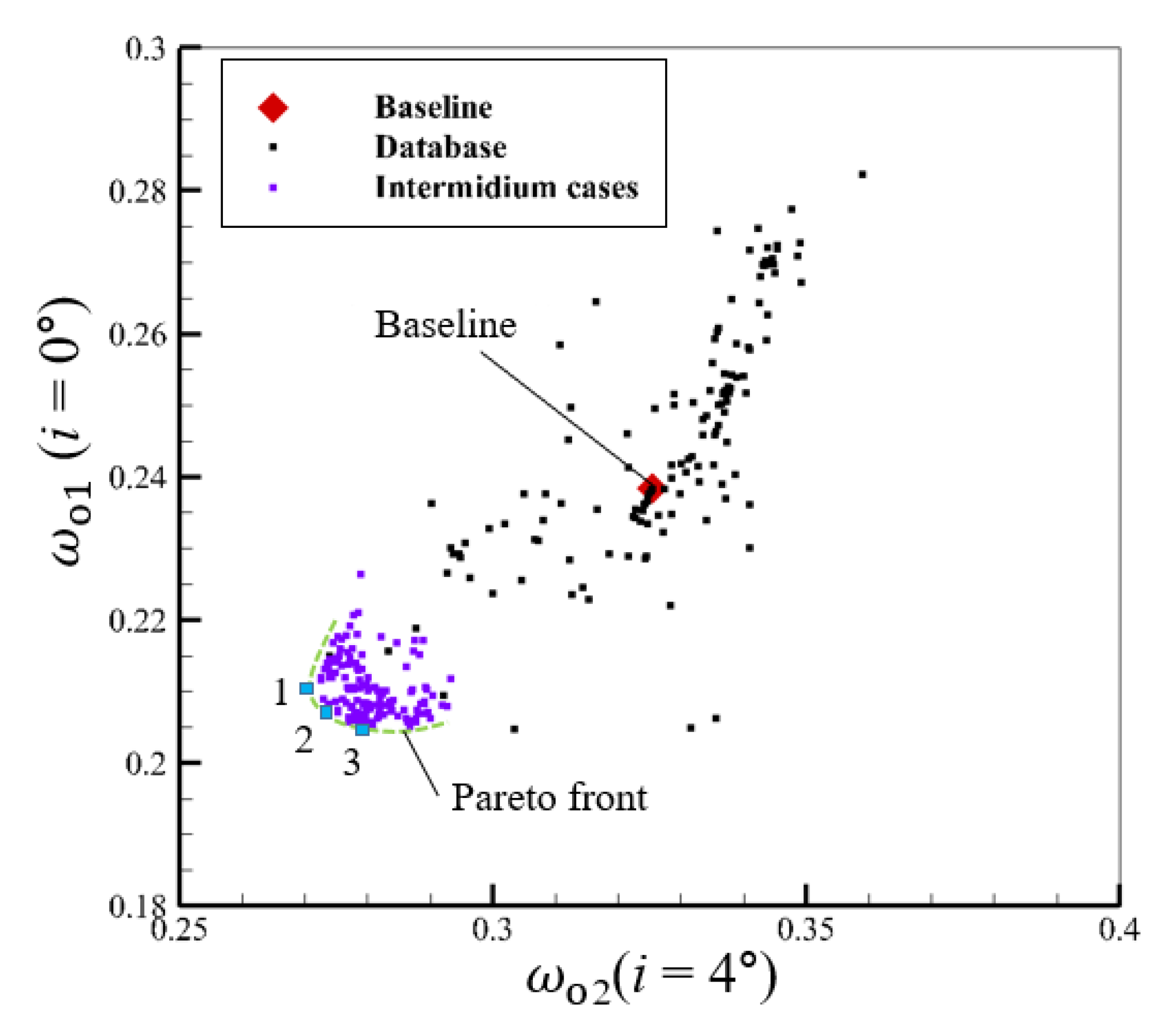
5.2. Analysis of Optimization Results and Overall Performance

The multi-objective optimization results are shown in Figure 12. The horizontal and vertical axes show the total pressure loss coefficients at OP2 and OP1. The black points represent the initial database samples, and the purple points represent the intermediate solutions of the optimization process. According to the direction of axes, samples at the lower-left corner represent the most effective NEWC cases at both OP1 and OP2. The green dashed curve indicates the Pareto front. Because it shows an acute angle, this means that, to some extent, the NEWC can simultaneously improve the performance at both OP1 and OP2. Here, we present three NEWC cases (labeled as 1, 2, and 3) near the Pareto front for further analysis, in which case 1 performs better at OP2, case 3 performs better at OP1, and case 2 shows a more balanced improvement. Note that (ω_o1, ω_o2) of the three cases are similar to each other, with a maximum difference of less than 0.01. Therefore, only the most balanced case of NEWC, i.e., case 2, was chosen for detailed analysis in the subsequent investigation. Figure 13 shows the contour of normalized height ($\overline{H}$) of case 2. The end wall was concave near the PS and convex near the SS. There was also a local fillet-like surface alongside the SS corner, with its start and end near the LE and TE, and a gentle streamwise slope in the upstream passage. It can be seen that the characteristics of case 2 agree with the conclusions of the correlation analysis very well.

Figure 14 compares the spanwise distribution of the total pressure loss coefficient(ω) and axial density flow ratio (AVDR) between the baseline cascade and case 2. AVDR is defined as:

$$AVDR=\frac{{\left.\rho (x)V_z(x)\right|}_{0.5C}}{{\left.\rho (x)V_z(x)\right|}_{\mathrm{inlet}}}$$

(14)

where the density(ρ) and axial velocity(V_z) at 0.5C should have the exact spanwise location as those of the inlet. In both operating points, Figure 14a shows that applying the NEWC decreases ω by up to 0.12 from the hub to 0.3span, which indicates the NEWC could significantly suppress the development of corner separation. Meanwhile, the value of AVDR decreases near 0.5span and increases near the hub, making AVDR approximately 1.0. This indicates that the end wall blockage due to the corner separation has been relieved by the NEWC.

To further illustrate the relationship between the loss variation and corner separation, a quantitative analysis was carried out based on the loss source model developed previously [20]. Assuming that the flow is constant, an open system control volume can be created for the computational domain of the cascade. Here, we define the control volume of the computational domain as v and the mass flow rate as ṁ. The subscript 1 and 2 represent the inlet and outlet, respectively. Then, the generation of loss within the control volume will result in lower mechanical energy at the outlet than at the inlet. The reduction of the overall total pressure due to the loss source in v can be calculated according to Equation (15):

$$\Delta P^{*}=P_1^{*}-P_2^{*}=P_1^{*}\left(1-{\left(\frac{T_1^{*}}{T_1^{*}-\frac{1}{\dot{m}CP}{\displaystyle \underset{v}{\iiint }\mathsf{\Phi }dv}}\right)}^{\frac{k}{k-1}}\right)$$

(15)

Note that the control volume in Equation (15) indicates the position when the dissipation occurs. Therefore, if using a particular control volume v_i instead of the overall control volume v, the reduction of total pressure calculated from Equation (15) would only correspond to the dissipation that occurs in v_i. For the losses in volume v_i, the contribution of a particular loss source to the change in total inlet/outlet pressure can be measured by:

$$L{S}_v=\frac{\Delta P_{\mathrm{v}}^{*}}{P_1^{*}-P_1}$$

(16)

Note that the denominator is the same as ω_o. The coefficient LS_v thus indicates the total pressure loss coefficient corresponding to the loss source in a particular control volume v_i.

Figure 15 shows the method of selecting the control volume to calculate the loss sources. Region 1 includes the flow field from −0.1C_a to 0.1C_a. Losses in this region originate mainly from an LE blockage. Therefore, the estimation of this loss source is defined as LS_LE. Loss in region 2 arises primarily from the friction between the blade surfaces and main flow, and the region is a skin-like volume around the blade surface downstream of 0.1C_a, with y⁺ below 200. This is defined as LS_BF. Region 3 includes the space taken out of region 2, spreading from 0.1C_a to the TE, where the generation of loss is mainly due to the dissipation loss of corner separation. The estimated value of this loss source is defined as LS_SU. Region 4 includes the space downstream of TE, where loss is generated from the mixing process between the main flow, secondary flow, and the corner separation. The loss source in this region is estimated and defined as LS_SD.

In addition, the kinetic energy of the secondary flow is defined as:

$$ske=\frac{1}{2}\rho {[\mathit{V}-(\mathit{V}\cdot {\mathit{n}}_{prim}){\mathit{n}}_{prim}]}^2$$

(17)

in which n_prim is the direction of the main flow. The total pressure loss result from secondary flow energy loss between the TE and the outlet can be defined as:

$$L{S}_{ske}=\frac{sk{e}_{TE}-sk{e}_{outlet}}{P_1*-P_1}$$

(18)

Therefore, the contribution of all separation loss within the cascade can be calculated by:

$$L{S}_{SEP}=L{S}_{SU}+L{S}_{SD}-L{S}_{ske}$$

(19)

Table 2. The estimation of loss sources of the baseline cascade.

Loss Sources	LSLE	LSBF	LSSU	LSSD	LSske	LSSEP
i = 0°	0.0744	0.0631	0.0418	0.0566	0.0017	0.0968
i = 4°	0.1065	0.0755	0.0561	0.0852	0.0025	0.1389

estimates the loss sources for the baseline cascade. It is clear that the LE loss (LS_LE) and separation loss (LS_SEP) dominate at OP1 and become more significant at OP2. The separation loss takes more than 41% of the total loss in both working conditions. Based on Table 2, changes in loss sources after applying the NEWC of case 2 are also calculated.

Table 3. The effect of NEWC on the loss sources.

	i = 0°	i = 4°
$(L{S}_{\mathrm{SEP},\mathrm{case}2}-L{S}_{\mathrm{SEP},\mathrm{baseline}})/{\displaystyle \sum L{S}_{\mathrm{baseline}}}$	−10.18%	−13.01%
$({\displaystyle \sum L{S}_{\mathrm{case}2}}-{\displaystyle \sum L{S}_{\mathrm{baseline}}})/{\displaystyle \sum L{S}_{\mathrm{baseline}}}$	−12.89%	−16%

gives the relative changes of the overall loss source and LS_SEP before and after using NEWC. The overall loss source is defined as:

$${\displaystyle \sum LS=L{S}_{LE}+}L{S}_{BF}+L{S}_{SU}+L{S}_{SD}$$

(20)

According to Table 3, the relative reduction of LS_SEP at OP1 reaches 10.18%, which takes 78% of the overall reduction (12.89%). For the situation in OP2, the reduction of LS_SEP at OP1 increases to 13.01%, similarly taking 81% of the overall reduction (16%). Apparently, the variation of separation loss is the major part of the overall effect of NEWC in both working conditions. This reveals that for the current cascade, the control of corner separation and the overall loss are simultaneous. Therefore, this confirms that the aim of the optimization process in Section 4, i.e., to minimize loss, nearly equals suppressing the corner separation. Thus, the following discussion associated with the variation of loss can be regarded as an indicator for the control of corner separation flow.

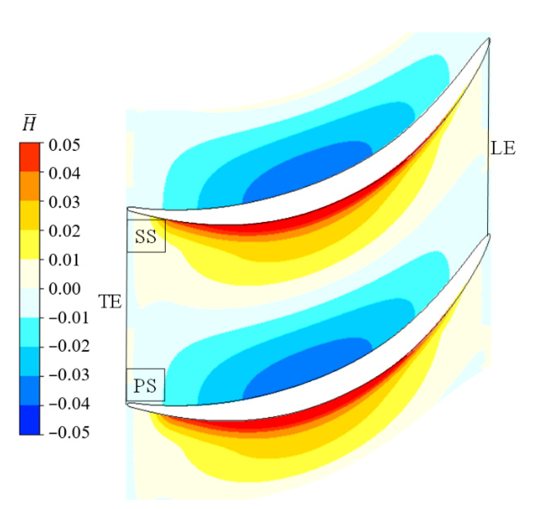
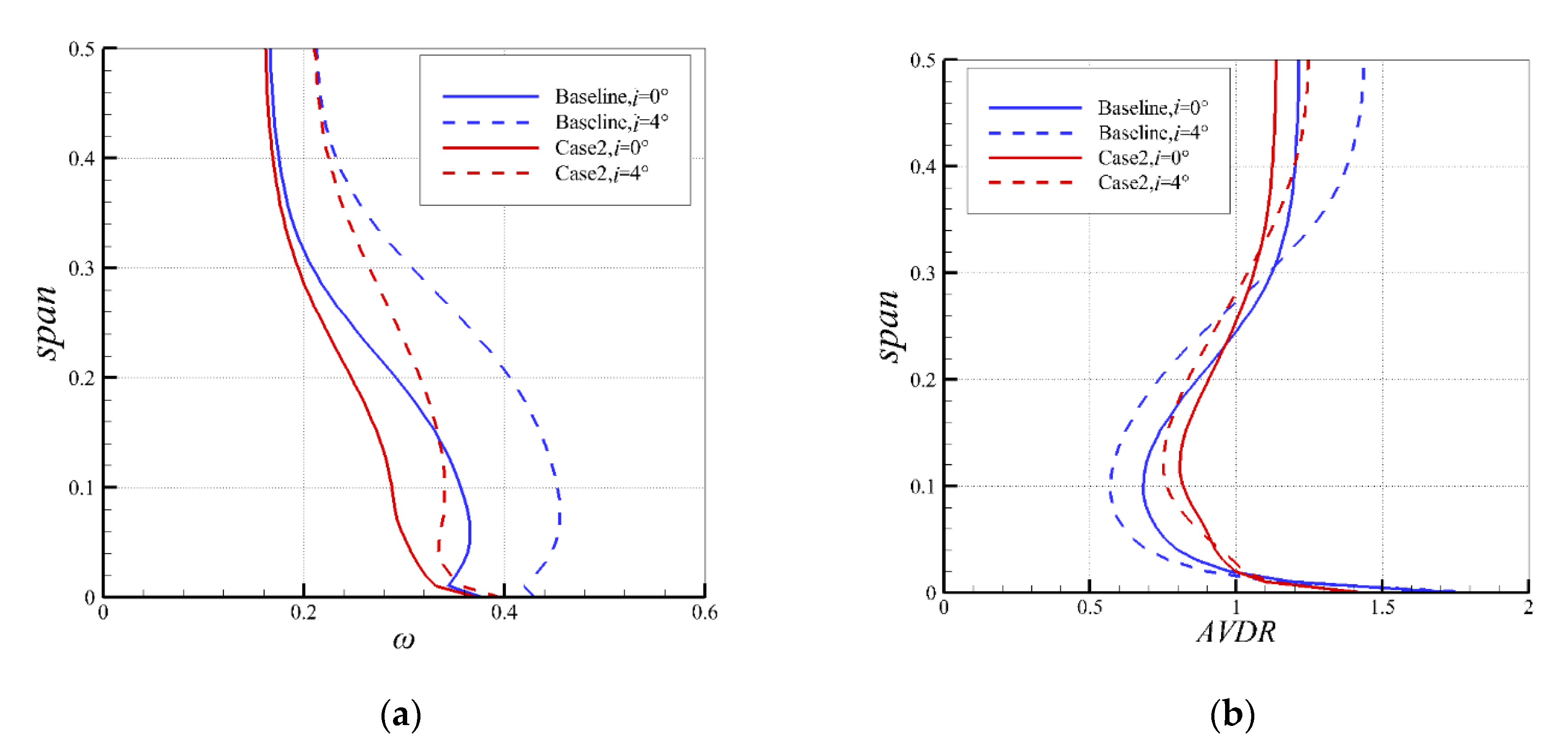
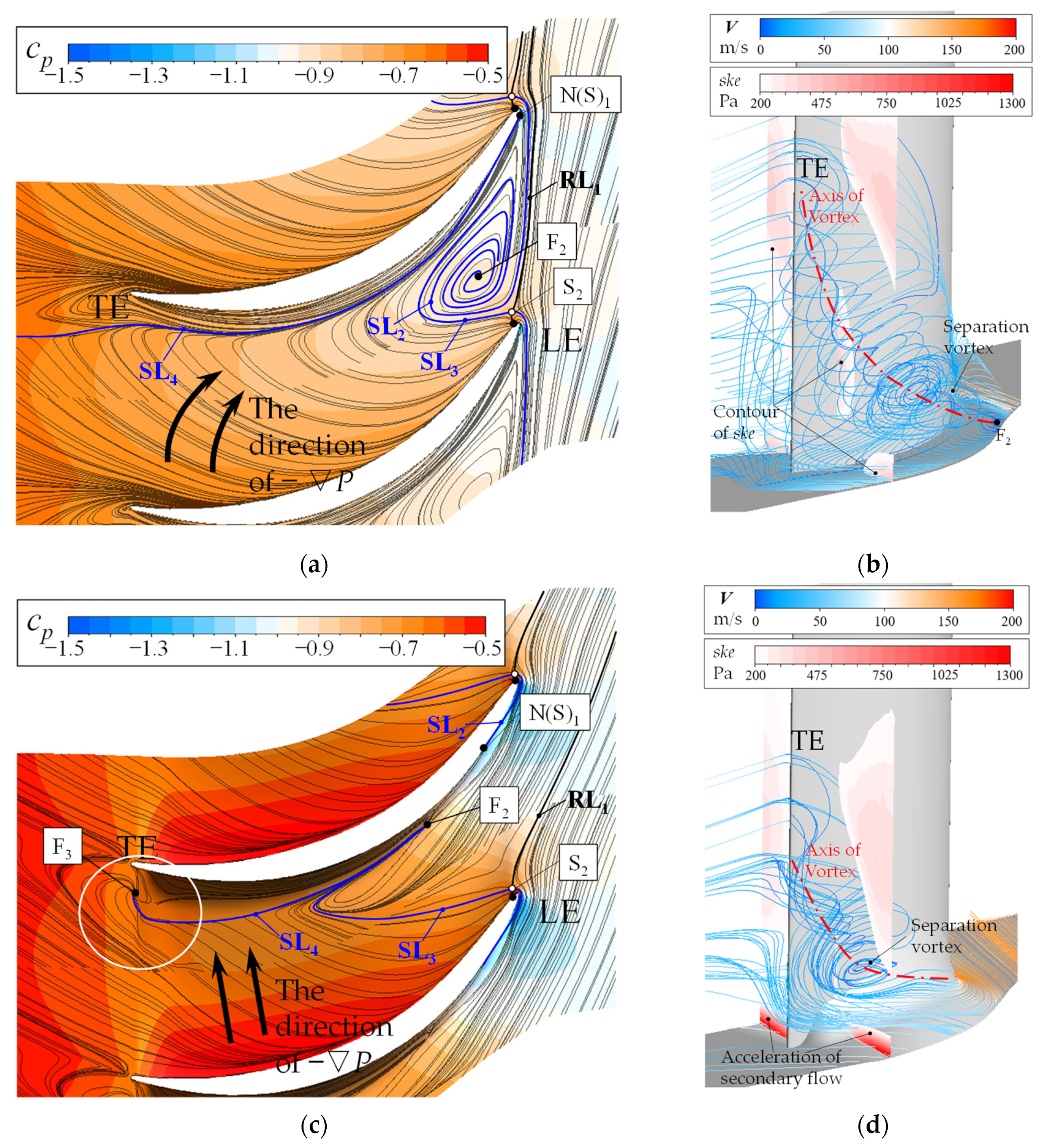
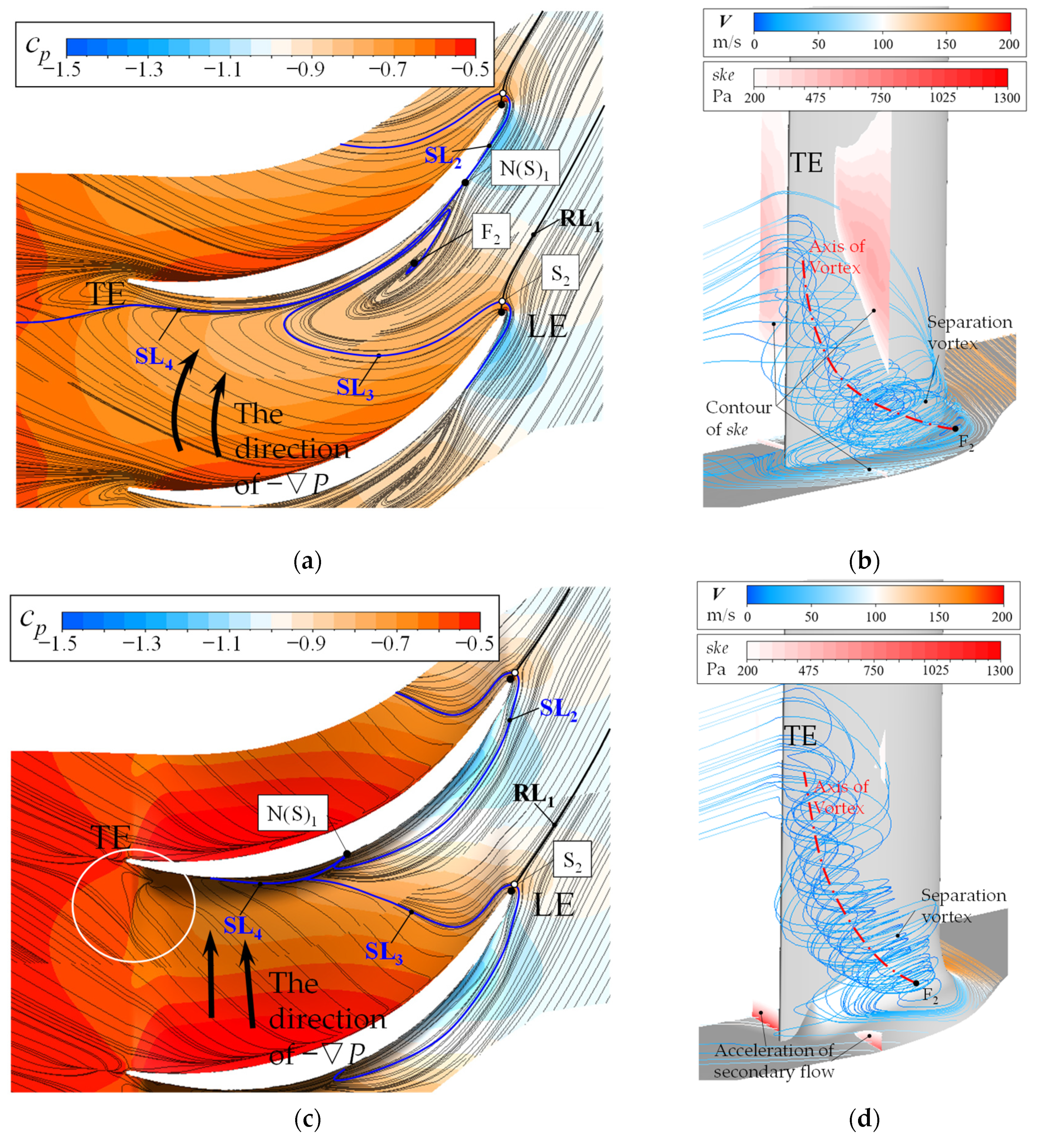
5.3. The Effect of NEWC on the Flow Field

To investigate the flow control rules of NEWC, Figure 16 and Figure 17 show the effect of NEWC on the loss distribution and the flow field, respectively. In Figure 16, the blue and red curves represent the streamwise growth rate of total pressure loss (ώ) before and after applying NEWC. The green curve represents the difference between them, meaning the improvement in reducing the growth rate of loss due to the NEWC. Figure 17 shows the limiting streamlines on the SS and illustrates the reverse flow region of corner separation using the iso-surface of V_z = 0 m/s (transparent surface). Section 5.2 indicates that compared with the design point, the corner separation is more severe at a high incidence, while the NEWC brings more benefits. Therefore, the following discussion will focus on the effect of NEWC at OP2, then we will compare it with the situation at OP1.

At OP2, Figure 16a shows that the highest ώ occurs near the LE. The NEWC increases ώ by 0.004 from −0.1C_a to LE but then decreases it more from the LE to 0.2C_a. The main cause of this decrease is the variation in flow structure near the LE of the cascade. Figure 17a shows that the semi-saddle point S(N)₁, which marks the onset of corner separation, is significantly shifted downstream. Therefore, the reverse flow region (downstream of the separation line SL₁) is consequently swept to the TE, which leads to a significant decrease in shear loss from LE to 0.2C_a. In the downstream region, the suppression of corner separation further reduces ώ by 0.002 on average from 0.2C_a to TE. Then, a second peak value occurs at 0.1C_a downstream of the TE, due to the dissipation of the shedding low energy fluid from the corner separation flow. Although the NEWC does not extend to this region, ώ is reduced by about 0.004 because of the relief of corner separation in its upstream blade passage.

At OP1, the cascade generates a higher peak of ώ near LE than at OP2. However, Figure 16b shows that applying the NEWC is much less effective in reducing the generation of loss from LE to 0.4C_a. As in the flow field of Figure 17b, applying the NEWC delays the onset of corner separation from 0.15C_a to 0.4C_a. However, because the reverse flow in the baseline cade is not widespread in the front of the blade passage, the benefit of the NEWC is not evident until 0.5C_a. In the rear part of the cascade, the average decrease in ώ is about 0.002. The effect of NEWC is similar to the situation in OP2, so we will not discuss this further to avoid redundant statements.

When applying NEWC, the above corner separation and loss variation are closely related to the motion of the end wall secondary flow. In the end wall region of the compressor, the flow motion is mainly driven by the end wall pressure gradient (▽P). When the NEWC changes the magnitude/direction of the original ▽P, the end wall secondary flow will be driven differently. The change in viscous force (τ) is more like an obstacle. The change in ▽P induced by the NEWC acts as the main driving force for the variation of the end wall secondary flow.

Figure 18 shows the contour of the end wall static pressure coefficient and limit streamlines. At OP2, the low-pressure region of the baseline cascade appears near the LE (Figure 18a). The end wall boundary layer separates strongly in the front passage, with the separation vortex core in the middle of the channel at 0.15C_a (labeled as F₂). The re-attachment line RL₁ from the inflow to the LE almost coincides with the separation line SL₂ emanating from the saddle point (S₂) of the adjacent LE. It can be seen that the separation vortex nearly blocks the entrance of the blade channel. Downstream of the separation line SL₃, the end wall secondary flow emanates from the PS and flows towards the mid-chord under the inverse pressure gradient, forming the reverse flow near the SS corner. Figure 18b further shows that the reverse flow near the LE of the SS is centered on the above end wall vortex point F2 in the three-dimensional flow field. After leaving the end wall surface, the end wall flow converges into the vortex structure and accumulates near the downstream SS to form the corner separation. The separation line SL₄ is the boundary of corner separation on the end wall surface.

When applying the NEWC, Figure 18c shows a significant improvement in the flow field near the front region of the SS corner. This improvement is partially due to the streamwise upslope of the end wall surface, which accelerates the inflow, thus shifting the end wall flow to the streamwise direction and delaying its accumulation to the SS. More importantly, this should be caused by the relief of corner separation, which removes the blockage in the front passage and enables the flow to enter the blade channel under the inverse pressure gradient smoothly. The main factor suppressing the above-mentioned corner separation is the variation of the end wall secondary flow downstream of the separation line SL₄. Figure 18c shows that −▽P turns to the SS in the rear passage (shown by the black arrows). As a result, the contour of ske in Figure 18d indicates that the end wall secondary flow is accelerated towards the SS while preserving its axial momentum. On the one hand, the acceleration of the end wall secondary flow significantly weakens the reverse corner flow, thus suppressing the spreading of corner separation in the front passage. On the other hand, this forces the corner separation to a relatively small area near the TE. The three-dimensional flow field of Figure 18d shows that after applying the NEWC, the axis of the separation vortex is shifted to the TE. The accumulation of low-energy fluid in the SS corner is reduced. According to previous studies [10,21], the local pitch-wise acceleration of the end wall secondary flow mixes with the low-energy separation fluid and improves its momentum, thus significantly reducing its dissipation loss in the high-speed main flow. In addition, near the TE, case 2 shows a higher streamwise pressure gradient (in the white circle). This is caused by the local diffusing of the end wall surface to ensure a smooth transition between NEWC and the downstream flat end wall. It seems to be a disadvantage but has never offset the positive contribution of the NEWC to the overall performance.

Figure 19a–d show the effect of NEWC at OP1. Compared with OP2, Figure 19a still shows the focus point (F₂) and the corresponding reverse flow between F₂ and SS. However, the F₂ stays more downstream than OP1 and approaches the SS, and there is no severe blockage in the front passage. Figure 19b shows that the separation vortex is emitted from F₂ and its axis is gradually approaching the TE of the SS. The three-dimensional separation flow around this vortex axis extends up to 0.25 span. Therefore, at the design point, the influence of corner separation mainly stays in the back half of the blade channel.

Figure 19c shows that the impact of NEWC on the flow field at OP1 is less significant than that of OP2 but still shows little essential difference. In the upstream SS corner, because the front passage is unblocked at this operating point, the variation of the flow field in the upstream passage clearly shows an improvement due to the streamwise upslope. The end wall boundary layer accelerates along the flow direction, pushes the reverse flow to 0.5C_a, and removes F₂ in the front passage. The most important effect is in enhancing the pitch-wise pressure gradient in the middle and rear regions of the blade channel. As a result, the end wall secondary flow in the rear blade channel is accelerated and is driven to the SS as in OP2. Figure 19d shows that the low-energy fluid in the corner separation is similarly shifted in the spanwise direction, consequently promoting the mixing effect between the secondary flow and the low-energy fluid. The negative effect of the transition between NEWC and the downstream end wall surface also exists (in the white circle in Figure 19c).

5.4. Summing-Up of the Effective End Wall Contouring Rules

With the above analysis, the effective end wall contouring rules and the corresponding corner separation control mechanism can be summarized, based on the current parametric method.

First, for the optimum end wall contouring case, the continuous unit should have a concave pressure side and convex suction side, while the localized unit should construct a local upslope to the SS, forming a fillet-like structure. It can be seen that the surface characteristics are highly consistent with the conclusions of the correlation analysis in Section 5.1. According to the flow field analysis, the function of the end wall contouring is to adjust the cross-passage pressure difference from the middle to the rear part of the channel, thus accelerating the rear-passage end wall’s secondary flow to the SS corner. As a result, the accelerated secondary flow reduces the spreading range of corner separation and mixes with the low energy fluid of separation flow, thus reducing its dissipation loss in the high-speed main flow. The above flow control positively affects corner separation both at the design point and with increasing incidence.

Second, the localized unit should form an upslope end wall in the front region of the SS corner. At the design point, this upslope accelerates the end wall boundary layer flow in the streamwise direction, so the local end wall flow contacts the SS in a more downstream position, while the separation vortex also moves rearward. When the incidence increases, the end wall contouring has removed the widely spreading corner separation. Therefore, compared to the effect of the upslope surface, it should be the removal of corner separation that primarily eliminates the blockage and accelerates the local end wall boundary layer flow. According to the correlation analysis, the axial starting point of the first localized unit (κ_s) is negatively correlated with the loss coefficient, indicating that a smaller distance between the axial starting point and the LE (i.e., a smaller κ_s) could help to reduce the overall loss. Besides this, the parameter of upstream slope (κ₁) is inversely correlated with the loss, indicating that a slower slope is beneficial. These are all consistent with the conclusions obtained from the flow field analysis.

Third, for the suction side of the end wall contouring near the TE, the optimized end wall surface falls back to ensure a smooth transition to the downstream end wall, thus leading to a local diffusing flow and triggering a strong inverse pressure gradient. The effect of this inverse pressure gradient on flow is negative. However, this disadvantage does not offset the benefit of the end wall contouring, either at the design point or with high incidence. The end wall contouring at the TE location is mainly related to the second localized unit. The correlation analysis shows that κ₂₁ has a negative correlation with the overall loss, i.e., the overall loss reduces when the end position of the end wall contouring approaches the TE, thus intensifying the TE diffusion. Therefore, both the flow field and the correlation analysis suggest that the negative influence of the end wall contouring near the TE is less significant than the benefit that the end wall contouring brings.

In summary, the correlation analysis and the flow field analysis clearly show that the new method is closely related to the flow control mechanism, and there is sufficient design space for optimization. The results show that the most effective flow control mechanisms are directly related to the control variables, making the rules of end wall contouring easy to establish. Its ability to effectively control the separation of the compressor corners is thus confirmed. All these demonstrate the superiority of the new end-wall modeling method in terms of parametric design.

6. Conclusions

With the aim of improving the control of the corner separation in the axial compressor, this paper proposes a new end wall contouring method and applies it in a numerical optimization design to verify its effectiveness on a high-load compressor cascade. According to the results and the discussion, the following can be concluded:

(1)

The idea behind the new end wall contouring method is to define multiple groups of end wall contouring units with different secondary flow control functions during the parameterization and then combine their flow control effects by applying a weighted superimposition of all the end wall contouring units. Compared with the previous studies, the new end wall contouring method enables the flexible combination of the control force from more than one position of the end wall surface.

(2)

The optimum end wall contouring presents a full-range end wall surface with a rising suction side and a sinking pressure side, while locally raising the end wall from the LE to the TE in the SS corner with a gentle upstream slope. The corresponding effect on the flow field is to adjust the pressure gradient from the middle to the rear part of the blade channel, to accelerate the end wall secondary flow when it reaches the SS corner. As a result, the accelerated secondary flow will suppress the spreading range of corner separation and, at the same time, reduce the dissipation loss between the low-energy separation flow and the high-speed main flow.

(3)

The design space of the new method is constructed with a relatively small number of control variables, but it contains sufficient effective solutions for controlling the corner separation. As a result, the optimization process reaches convergence with a relatively shorter computing time than the traditional method. The optimal design reduces the total pressure loss coefficient of the high-load cascade by 5% at the design point and by 3% when the incidence is increased. The numerical results confirm its effectiveness in controlling corner separation with multiple operating points, regardless of the significant difference in the development of corner separation. There is also a clear relationship between flow control and parameter settings. This finding thus indicates the advantage of the newly developed end wall contouring method compared with previous studies.

References

1. Koff, B.L. Gas Turbine Technology Evolution: A Designers Perspective. J. Propuls. Power 2004, 20, 577–595. [Google Scholar] [CrossRef]
2. Liu, B.; An, G.; Yu, X. Experimental investigation of the effect of rotor tip gaps on 3D separating flows inside the stator of a highly loaded compressor stage. Expl. Therm. Fluid. Sci. 2016, 75, 96–107. [Google Scholar] [CrossRef] [Green Version]
3. Fei, T.; Ji, L.; Yi, W. Investigation of the Dihedral Angle Effect on the Boundary Layer Development Using Special-Shaped Expansion Pipes. In Proceedings of the ASME Turbo Expo, Oslo, Norway, 11–15 June 2018. GT2018-76383. [Google Scholar]
4. Taylor, J.V.; Miller, R.J. Competing 3D Mechanisms in Compressor Flows. Vol. 7b Struct. Dyn. 2015, 139, 021009. [Google Scholar] [CrossRef]
5. Lei, V.-M.; Spakovszky, Z.S.; Greitzer, E.M. A Criterion for Axial Compressor Hub-Corner Stall. J. Turbomach. 2008, 130, 031006. [Google Scholar] [CrossRef] [Green Version]
6. Li, X.; Chu, W.; Zhang, H. Investigation on relation between secondary flow and loss on a high loaded axial-flow compressor cascade. J. Propul Technol. 2014, 35, 914–925. [Google Scholar]
7. Rose, M.G. Non-Axisymmetric Endwall Profiling in the HP NGV’s of an Axial Flow Gas Turbine. In Proceedings of the ASME 1994 International Gas Turbine and Aeroengine Congress and Exposition, The Hague, The Netherlands, 13–16 June 1994; American Society of Mechanical Engineers Digital Collection: New York, NY, USA, 1994. [Google Scholar] [CrossRef] [Green Version]
8. Brennan, G.; Harvey, N.W.; Rose, M.G.; Fomison, N.; Taylor, M.D. Improving the Efficiency of the Trent 500-HP Turbine Using Nonaxisymmetric End Walls—Part I: Turbine Design. J. Turbomach. 2003, 125, 497–504. [Google Scholar] [CrossRef]
9. Hu, S.; Lu, X.; Zhang, H.; Zhu, J.; Xu, Q. Numerical investigation of a high-subsonic axial-flow compressor rotor with non-axisymmetric hub endwall. J. Therm. Sci. 2010, 19, 14–20. [Google Scholar] [CrossRef]
10. Harvey, N.W. Some Effects of Non-Axisymmetric End Wall Profiling on Axial Flow Compressor Aerodynamics: Part I—Linear Cascade Investigation. In Proceedings of the ASME Turbo Expo 2008: Power for Land, Sea, and Air, Berlin, Germany, 9–13 June 2008; American Society of Mechanical Engineers Digital Collection: New York, NY, USA, 2008; pp. 543–555. [Google Scholar] [CrossRef]
11. Meng, T.; Yang, G.; Zhou, L.; Ji, L. Full blended blade and endwall design of a compressor cascade. Chin. J. Aeronaut. 2021, 34, 79–93. [Google Scholar] [CrossRef]
12. Harvey, N.W.; Offord, T.P. Some Effects of Non-Axisymmetric End Wall Profiling on Axial Flow Compressor Aerodynamics: Part II—Multi-Stage HPC CFD Study. In Proceedings of the ASME Turbo Expo 2008: Power for Land, Sea, and Air, Berlin, Germany, 9–13 June 2008; American Society of Mechanical Engineers Digital Collection: New York, NY, USA, 2008; pp. 557–569. [Google Scholar] [CrossRef]
13. Reising, S.; Schiffer, H.-P. Non-Axisymmetric End Wall Profiling in Transonic Compressors—Part I: Improving the Static Pressure Recovery at Off-Design Conditions by Sequential Hub and Shroud End Wall Profiling. In Proceedings of the ASME Turbo Expo 2009: Power for Land, Sea, and Air, Orlando, FL, USA, 8–12 June 2009; American Society of Mechanical Engineers Digital Collection: New York, NY, USA, 2009; pp. 11–24. [Google Scholar] [CrossRef]
14. Reising, S.; Schiffer, H.-P. Non-Axisymmetric End Wall Profiling in Transonic Compressors—Part II: Design Study of a Transonic Compressor Rotor Using Non-Axisymmetric End Walls—Optimization Strategies and Performance. In Proceedings of the ASME Turbo Expo 2009: Power for Land, Sea, and Air, Orlando, FL, USA, 8–12 June 2009; American Society of Mechanical Engineers Digital Collection: New York, NY, USA, 2009; pp. 25–37. [Google Scholar] [CrossRef]
15. Lepot, I.; Mengistu, T.; Hiernaux, S. Highly Loaded LPC Blade and Non Axisymmetric Hub Profiling Optimization for En-hanced Efficiency and Stability. In Proceedings of the ASME Turbo Expo, British Columbia, BC, Canada, 6–10 June 2011. GT2011-46261. [Google Scholar]
16. Dorfner, C.; Hergt, A.; Nicke, E.; Moenig, R. Advanced Nonaxisymmetric End wall Contouring for Axial Compressors by Generating an Aerodynamic Separator—Part I: Principal Cascade Design and Compressor Application. J. Turbomach. 2011, 133, 021026. [Google Scholar] [CrossRef]
17. Hergt, A.; Dorfner, C.; Steinert, W.; Nicke, E.; Schreiber, H. Advanced Non-axisymmetric End wall Contouring for Axial Compressors by Generating an Aerodynamic Separator—Part II: Experimental and Numerical Cascade Investigation. J. Tur-Bomach 2011, 133, 021027. [Google Scholar]
18. Reutter, O.; Hemmert-Pottmann, S.; Hergt, A.; Nicke, E. Endwall Contouring and Fillet Design for Reducing Losses and Homogenizing the Outflow of a Compressor Cascade. In Proceedings of the ASME Turbo Expo 2014: Turbine Technical Conference and Exposition, Düsseldorf, Germany, 16–20 June 2014; American Society of Mechanical Engineers Digital Collection: New York, NY, USA, 2014. [Google Scholar] [CrossRef]
19. Varpe, M.K.; Pradeep, A.M. Benefits of non-axisymmetric endwall contouring in a compressor cascade with a tip clearance. J. Fluids. Eng. 2015, 137, 051101. [Google Scholar] [CrossRef]
20. Li, X.; Chu, W.; Wu, Y. Numerical investigation of inlet boundary layer skew in axial-flow compressor cascade and the cor-responding non-axisymmetric end wall profiling. J. Power Energy 2014, 228, 638–656. [Google Scholar] [CrossRef]
21. Li, X.; Chu, W.; Wu, Y.; Zhang, H.; Spence, S. Effective end wall profiling rules for a highly loaded compressor cascade. Proc. Inst. Mech. Eng. Part A J. Power Energy 2016, 230, 535–553. [Google Scholar] [CrossRef] [Green Version]
22. Chu, W.; Li, X.; Wu, Y.; Zhang, H. Reduction of end wall loss in axial compressor by using non-axisymmetric profiled end wall: A new design approach based on end wall velocity modification. Aerosp. Sci. Technol. 2016, 55, 76–91. [Google Scholar] [CrossRef]
23. Li, X.; Dong, J.; Chen, H.; Lu, H. The Control of Corner Separation with Parametric Suction Side Corner Profiling on a High-Load Compressor Cascade. Aerospace 2022, 9, 172. [Google Scholar] [CrossRef]
Figure 1. The basic concept of the new end wall contouring method.
Energies 15 03305 g001
Figure 2. The continuous unit. (a) Definition of the continuous unit; (b) the effect on the pressure field and the end wall secondary flow.
Energies 15 03305 g002
Figure 3. The localized unit. (a) Definition of the localized unit; (b) the effect on the pressure field and the end wall secondary flow.
Energies 15 03305 g003
Figure 4. The effect of the weight factor on the characteristics of end wall contouring.
Energies 15 03305 g004
Figure 5. Mapping from the standard space to the end wall region of a compressor passage.
Energies 15 03305 g005
Figure 6. The geometry parameters of the baseline cascade.
Energies 15 03305 g006
Figure 7. Overview of the mesh.
Energies 15 03305 g007
Figure 8. The pitch-averaged total pressure loss coefficient at 0.5C downstream of the TE. (a) OP1, i = 0°; (b) OP2, i = 4°.
Energies 15 03305 g008
Figure 9. The experimental and CFD results of the static pressure coefficient on the end wall surface: (a) OP1, i = 0°; (b) OP2, i = 4°.
Energies 15 03305 g009
Figure 10. The framework of the optimization process.
Energies 15 03305 g010
Figure 11. Correlation analysis between control variables and overall total pressure loss. (a) OP2, i = +4°; (b) OP2, i = 0°. (c) The schematic plot of the variation of the end wall contouring units, due to the design variables.
Energies 15 03305 g011
Figure 12. The total pressure loss of NEWC samples during the optimization process.
Energies 15 03305 g012
Figure 13. The normalized height contour of the optimal case (case 2).
Energies 15 03305 g013
Figure 14. Comparison of the spanwise distribution of ω and AVDR before and after end wall contouring at 0.5C downstream of the TE. (a) ω; (b) AVDR.
Energies 15 03305 g014
Figure 15. The selection of control volume to calculate the loss sources.
Energies 15 03305 g015
Figure 16. The streamwise distribution of the growth rate of total pressure loss before and after applying NEWC; (a) OP2, i = 4°; (b) OP1, i = 0°.
Energies 15 03305 g016
Figure 17. The three-dimensional flow field before and after applying the NEWC: (a) OP2, i = 4°; (b) OP1, i = 0°.
Energies 15 03305 g017aEnergies 15 03305 g017b
Figure 18. The comparison of the three-dimensional flow field before and after applying the NEWC at OP2, i = 4°: (a) the end wall secondary flow of the baseline cascade; (b) the three-dimensional flow field of the baseline cascade; (c) the end wall secondary flow of case 2; (d) the three-dimensional flow field of the baseline cascade.
Energies 15 03305 g018
Figure 19. The comparison of the three-dimensional flow field before and after applying the NEWC at OP1, i = 0°: (a) the end wall secondary flow of the baseline cascade; (b) the three-dimensional flow field of the baseline cascade; (c) the end wall secondary flow of case 2; (d) the three-dimensional flow field of the baseline cascade.
Energies 15 03305 g019