IBM-LBM-DEM Study of Two-Particle Sedimentation: Drafting-Kissing-Tumbling and Effects of Particle Reynolds Number and Initial Positions of Particles

Abstract

Particle sedimentation is a fundamental process encountered in various industrial applications. In this study, we used immersed boundary lattice Boltzmann method and discrete element method (IBM-LBM-DEM) to investigate two-particle sedimentation. A lattice Boltzmann method was used to simulate fluid flow, a discrete element method was used to simulate particle dynamics, and an immersed boundary method was used to handle particle–fluid interactions. Via the IBM-LBM-DEM, the particles collision process in fluid or between rigid walls can be calculated to capture the information of particles and the flow field more efficiently and accurately. The numerical method was verified by simulating settling of a single three-dimensional particle. Then, the effects of Reynolds number (Re), initial distance, and initial angle of particles on two-particle sedimentation were characterized. A specific focus was to reproduce, analyze, and define the well-known phenomenon of drafting-kissing-tumbling (DKT) interaction between two particles. Further kinematic analysis to define DKT is meaningful for two-particle sedimentation studies at different particle locations. Whether a pair of particles has experienced DKT can be viewed from time plots of the distance between the particles (for kissing), the second-order derivative of distance to time (for drafting), and angular velocities of particles (for tumbling). Simulation results show that DKT’s signatures, including attraction, (near) contact, rotation, and in the end, separation, is only completely demonstrated when particles have nearly vertically aligned initial positions. Hence, not all initial positions of particles and Reynolds numbers lead to DKT and not all particle–particle hydrodynamic interactions are DKT. Whether particle–particle interaction is attractive or repulsive depends on the relative positions of particles and Re. Collision occurs when Re is high and the initial angle is small (<20°), almost independent of the initial distance.

1. Introduction

Particle sedimentation exists in many natural and engineering systems and is a classical problem in fluid mechanics and energy science. Resolved simulation of particle movement in sedimentation is of great importance for in-depth understanding and modeling of particle sedimentation [1,2]. While both experiments and resolved simulations may be used to investigate the complex particle-fluid dynamics in sedimentation, information that can be extracted from experiments is usually limited to particles’ positions and velocities and the velocity of the fluid phase when particle imaging velocimetry (PIV) is used. Particle-resolved numerical simulation, on the other hand, can provide many more details and is more suitable for studying the details of the flow field and the history of fluid-particle acceleration.

Sedimentation of one, two, and several particles has long been used to test the accuracies of particle-resolved simulations [3]. When particles are settling with moderate Reynolds numbers, their pairwise drafting-kissing-tumbling (DKT) interaction, first discovered experimentally by Fortes et al. [4], is classical for particle-resolved simulations to reproduce. Here, the Reynolds number is defined as Re = ud/ν where u is particle velocity, d is particle diameter, and ν is the kinematic viscosity of the fluid. Feng et al. [5] used a two-dimensional finite element method to simulate the sedimentation of circular and elliptic particles in a Newtonian fluid and put forward five modes of sedimentation with Re between 0 and 600. Patankar et al. [6] simulated settling of two two-dimensional particles using a distributed Lagrange-multiplier-based fictitious-domain method (DLM). Following the simulation conditions of Patankar et al., several research teams used different numerical methods to simulate DKT. Niu et al. [7] and Feng et al. [8] used an immersed boundary method-lattice Boltzmann method (IBM-LBM) scheme. The IBM coupled fluid and particle motions and LBM was used over the entire computational domain. Jafari et al. [9] simulated DKT using an LBM combined with a smoothing-profile method. Wang et al. [10] simulated DKT using a two-dimensional multiple-relaxation-time (MRT) LBM, in which the solid boundary was explicitly implemented. The no-slip boundary condition was recovered using the bounce-back method of Ladd and Verberg [11]. Hu et al. [12] developed a finite-volume LBM with modified fluid–particle momentum exchange and simulated DKT. Cao et al. [13] studied the influence of the initial angle and the distance on the interaction between two spherical particles in a 3D channel by using the lattice-Boltzmann method with discrete external boundary force and pointed out that two particles existed in three states, named repulsion, attraction, and transition (Re ≈ 100), and the smaller the initial angle the more likely the interaction is a repulsion. Liu et al. [14] proposed an improved curved boundary condition (CBC) for two-particle sedimentation in their latest study and compared their results with Niu et al. [7] and Hu et al. [12]. The overall agreement was good, except that the particle separation distance in Liu et al. [14] was slightly higher than those in Niu et al. [7] and Hu et al. [12]. The above studies on two-particle sedimentation were mostly based on the conditions of Patankar et al. [6], and the results of these studies were quite close.

The dynamics of particles in two-dimensional simulations and that in three-dimensional simulations are different. Nie et al. [15] proposed that the extra dimension allows different patterns of particle motion and new features of fluid–particle system to exist. Three-dimensional numerical simulation and limited experimental study presented by Dash et al. [16] on the sedimentation of two inline spheres showed that 2D particles settling in narrow channel experienced repeated DKT process that was not revealed in 3D study. Many scholars have made great efforts to study the influencing factors of the interaction between particles in the process of particle sedimentation. Among which, Dash et al. [16] believed that normalized trajectories, settling velocities and hydrodynamic force coefficients of sediment spheres are independent of Re (in the range of 10–60). It is also believed that particle size was a significant factor [15,17,18]. Nie et al. [19] found that the effect of particle density ratio cannot be ignored due to the effect of inertia on the motion of the particles. Studies have also been carried out to characterize the role of various influencing factors of the settlement of two particles, including thermal characteristics of particles [18], particle surface slip [20], cohesive forces during particle–particle interactions [21,22], and adhesion [23]. Liu et al. [24] proved that the settlement process is dominated by the viscous effect when Re is less than 60 and dominated by vortex interaction when Re becomes greater.

From this review, we note that in most previous studies on DKT, researchers paid attention to the properties of the particles on the interaction between particles. However, the dynamics of DKT are not only controlled by density ratio and Re, but also the initial positions of the particles. The combined effect of the initial positions, density ratio, and Re representing particle inertia and fluid viscous effects has not been thoroughly studied. In addition, as a classical phenomenon of the interaction between two particles, DKT defines the motion process of two particles in tandem. Further kinematic analysis to investigate similar DKT at any particle location is necessary to develop a DKT definition applicable to different particle locations.

From the research scale of particle fluid two-phase flow, there is macro-scale continuum theory, mesoscale lattice Boltzmann method, and micro-scale molecular dynamics. The consumption of computing resources increases sharply with the decrease of the research scale. The traditional numerical simulation used the solving of the Navier-Stokes equation coupled with DEM to study the motion of particles in a fluid [25,26]. A recent study that used this method was by Karvelas et al. [27]. They used the Navier-Stokes equation to calculate the fluid phase together with a Lagrangian model and track the particles in the discrete phase to study the aggregation formation and magnetic driving of spherical particles. The LBM developed in recent years is different from the traditional method. It has both the efficiency in the order of macro hydrodynamics and the accuracy in the order of micro molecular dynamics. Meanwhile, this method has a powerful parallel processing ability and can improve the computational efficiency of the numerical simulation. Immersed boundary method of fluid–structure interaction allows for nonconforming discretizations of the fluid and structure. This avoids the frequent re-meshing that is required by the body-conforming discretization method [28]. In the IBM, the effect of a solid boundary on fluid flow is reproduced by distributing force terms to the flow field, and the solid boundary is represented discretely by the Lagrange points. The flow equation is still solved over the entire computational domain [29]. As a simple and efficient boundary treatment method, IBM has a natural affinity with LBM due to the use of Euler nodes to simulate the flow field. Via the discrete element method (DEM) coupled with the IBM-LBM method, the collision process between fluid or rigid walls can be calculated to capture the information of particles and flow field more efficiently and accurately.

In this paper, we used two methods, LBM with an explicitly implemented solid boundary over which bounce-back is exercised (LBM-BB) and IBM with LBM and DEM (IBM-LBM-DEM), to simulate DKT of three-dimensional particles. In Section 2, we presented the details of these two numerical methods. IBM-LBM-DEM coupling is realized by compiling open-source codes. The main program takes the LBM C++ library (Palabos) and calls the DEM open source library (LIGGGHTS) to solve the dynamics of fluid and that of the particles. In Section 3, we used LBM-BB and IBM-LBM-DEM to simulate single-particle sedimentation and DKT. By reproducing known and published results, the accuracy of the two methods was proved. In Section 4, a specific focus was to reproduce, analyze, and define the well-known phenomenon of drafting-kissing-tumbling (DKT) interaction between two particles. Furthermore, sedimentations of two particles were initiated at different positions and angles with different Re numbers. Section 5 summarized the contributions of this work.

2. Model Descriptions

2.1. Lattice Boltzmann Method

In LBM, the fluid domain is divided into discrete Cartesian grids. In this paper, the lattice BGK (LBGK) method proposed by Chen and Qian [30,31] is used. The discrete velocity model is D3Q19, and the half-way bounce back method described in Ladd and Verberg [10] is used at the wall boundary.

In this paper, the evolution equation for the discrete velocities is:

$$f_i\left(\mathit{x}+{\mathit{c}}_i{\delta }_t,t+{\delta }_t\right)-f_i\left(\mathit{x},t\right)=-\frac{1}{\tau }\left[f_i\left(\mathit{x},t\right)-f_i^{eq}\left(\mathit{x},t\right)\right]$$

(1)

where $f_i\left(\mathit{x},t\right)$ is the velocity distribution at spatial position x and time t in the direction i, τ is the relaxation time, ${\Omega }^f=\left(f_i^{eq}-f_i\right)/\tau$ is the fluid collision operator in BGK model, $f_i^{eq}\left(\mathit{x},t\right)$ is the equilibrium velocity distribution at x and t in the direction of i, c_i is $f_i$’s corresponding lattice velocity, ${\delta }_t$ is the streaming time step, and $f_i\left(\mathit{x}+{\mathit{c}}_i{\delta }_t,t+{\delta }_t\right)$ is the distribution at spatial position $\mathit{x}+{\mathit{c}}_i{\delta }_t$ and time $t+{\delta }_t$ in the direction of i. The equilibrium distribution is

$$f_i^{eq}=w_i{\rho }_f\left[1+\frac{{\mathit{c}}_i·{\mathit{u}}_f}{c_s^2}+\frac{{\left({\mathit{c}}_i·{\mathit{u}}_f\right)}^2}{2c_s^4}-\frac{u_f^2}{2c_s^2}\right]$$

(2)

The discrete velocity of the D3Q19 model is

$$c_i=c\left[\begin{array}{ccccccccccccccccccc}0& 1& -1& 0& 0& 0& 0& 1& -1& 1& -1& 1& -1& 1& -1& 0& 0& 0& 0\\ 0& 0& 0& 1& -1& 0& 0& 1& -1& -1& 1& 0& 0& 0& 0& 1& -1& 1& -1\\ 0& 0& 0& 0& 0& 1& -1& 0& 0& 0& 0& 1& -1& -1& 1& 1& -1& -1& 1\end{array}\right]$$

(3)

The weighting coefficients of the D3Q19 model are:

$$c_s=\frac{c}{\sqrt{3}},w_i=\{\begin{array}{l}1/3 c_i^2=0 \\ 1/18 c_i^2=c^2\\ 1/36 c_i^2=2c^2\end{array}$$

(4)

$c_s$ is referred to as the lattice sound velocity, c = dx/dt is the lattice speed, dx is the lattice length unit that represents the spacing between two lattice nodes, dt is the lattice Boltzmann time step, and $w_i$ is the weighting coefficient. The local density is ${\rho }_f={\displaystyle \sum _i{f}_i}$ and the local fluid momentum is ${\rho }_f{\mathit{u}}_f={\displaystyle \sum _i{f}_i}{c}_i$. The relaxation time parameter τ controls the kinematic viscosity $\nu$ of the fluid:

$$\nu =c_s^2\left(\tau -\frac{1}{2}\right)\frac{{\delta }_x^2}{{\delta }_t}$$

(5)

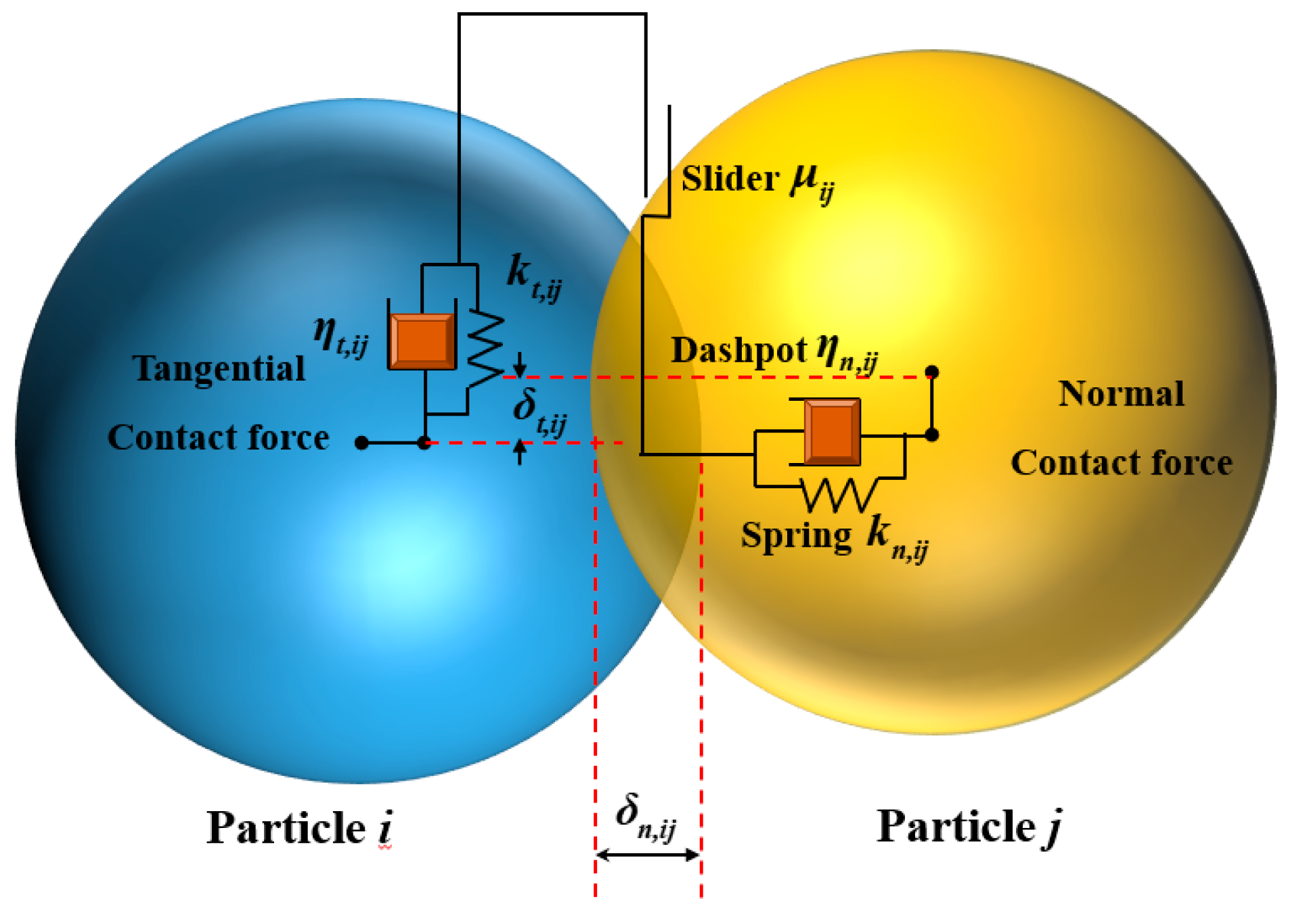
2.2. Discrete Element Method

In DEM, particles are discrete entities, each of which possesses its momentum and angular momentum equations [32]. In this study, forces and torques used to update particles’ velocity and angular velocity are from particle–particle contact, gravity, and particle–fluid interaction [33]. The specific equations are:

$$m_p\frac{\mathrm{d}{\mathit{v}}_p}{\mathrm{d}t}=m_p\mathit{g}+{\mathit{F}}_c+{\mathit{F}}_f$$

(6)

$$I_p{\mathit{\omega }}_p={\mathit{T}}_c+{\mathit{T}}_f$$

(7)

where $m_p$ is particle mass, ${\mathit{v}}_p$ is particle velocity, ${\mathit{\omega }}_p$ is particle angular velocity, $I_p$ is particle moment of inertia, ${\mathit{F}}_c$ is the net force from particle–particle contact, ${\mathit{T}}_c$ is the net torque from particle–particle contact. ${\mathit{F}}_f$, the net force from the fluid, and ${\mathit{T}}_f$, the net torque generated by fluid–solid interaction, will be presented in Section 2.3 as they are parts of the IBM.

${\mathit{F}}_c$ and ${\mathit{T}}_{\mathrm{c}}$ were calculated using the soft sphere model [34]. In this model, interactions between spherical particles are modeled as a combination of elastic and frictional contacts. The normal force between particles is generated by a spring and a damper, and the tangential force is generated by a spring, a damper, and a slider (Figure 1). A small overlap is allowed between the particles, based on which the normal force and the tangential force are calculated. The soft sphere model is particularly effective in handling dense particle flows where multi-body contacts occur frequently.

The net contact force is decomposed into the normal contact force (${\mathit{F}}_{ij}^n$) and the tangential contact force (${\mathit{F}}_{ij}^t$) in the soft sphere model. A Hertz model [35] was adopted to describe the elastic parts of normal and tangential forces generated during particle–particle contacts.

$${\mathit{F}}_c={\displaystyle {\sum }_{j=1,j\ne i}^N\left({\mathit{F}}_{ij}^n+{\mathit{F}}_{ij}^t\right)}$$

(8)

The normal contact force between particle i and particle j is calculated as

$${\mathit{F}}_{ij}^n=k_n{\delta }_n-{\eta }_n\Delta {\mathit{v}}_{n,ij}$$

(9)

where ${\delta }_n$ is the length of overlap along the normal direction, k_n is the coefficient of stiffness in the normal direction, η_n is the normal damping coefficient, and $\Delta {\mathit{v}}_{n,ij}$ is the relative normal velocity between the particles. The tangential contact force is calculated similarly as

$${\mathit{F}}_{ij}^t=k_t{\delta }_t-{\eta }_t\Delta {\mathit{v}}_{t,ij}$$

(10)

where ${\delta }_t$ is the length of the tangential overlap. The production k_tδ_t produces tangential elastic restitution; ${\delta }_t$ is specifically calculated by integrating the relative tangential velocity throughout the contact. k_t is the coefficient of stiffness in the tangential direction, η_t is the tangential damping coefficient, and $\Delta {\mathit{v}}_{t,ij}$ is the relative tangent velocity between the particles. The tangential overlap is truncated to fulfill ${\mathit{F}}_{ij}^t\le {\mu }_{ij}{\mathit{F}}_{ij}^n$.

The handling of particle and wall interactions requires special instructions. Bound the simulation domain of a system with a frictional wall. All particles interact with the wall when they are close enough to touch it. The equation for the force between the wall and particles touching it is the same as the corresponding equation, in the limit of one of the two particles going to infinite radius and mass.

2.3. Immersed Boundary Method

There are two different IB calculation schemes, called kinematic IB scheme and dynamic IB scheme, which were used to impose boundary conditions on immersed geometry [36,37]. The kinematic IB method considered the influence of the object on the surrounding fluid through the forced term obtained from the solid boundary, and added its influence to the fluid. This is a traditional method which can be accurately applied to the no slip boundary. Di [1], Feng [8], Dash [16], Yang [18], and others adopted this scheme when dealing with the geometry boundary. The dynamic IB scheme determined the contribution of hydrodynamic external force and structural internal force by Newton’s second law. It has more advantages for applying acceleration boundary conditions [38]. Therefore, this format was adopted in the research of Niu [7], Hu [12], and Cao [13]. Existing research results showed that the two schemes agree well for low capillary numbers. The dynamic IB scheme has a stronger prediction ability in the geometry of inertial and non-inertial deformation. Therefore, the dynamic IB scheme was selected in this paper.

For LBM-IBM in this paper, it is on the Eulerian points that the velocity distribution is defined. Over and across the fluid–particle boundary immersed in lattice cells, the collision operator Ω becomes dependent on the local solid ratio ε (1 in solid cells, 0 in fluid cells, and boundary cells 0 < ε < 1). The solid ratio of the boundary cell is further solved by a lattice decomposition. As shown in Figure 2, a two-dimensional boundary cell is subdivided into 5 × 5 decomposition cells. If the distance from a decomposition cell to the center of the sphere is greater than the radius of the sphere, the decomposition cell is considered as a fluid cell; if the distance from the cell to the center of the sphere is less than the radius, the cell is considered as a solid cell. Using this method, the solid ratio of the boundary cell is determined.

When solid ratio ε is zero, regular collision operator Ω_f is used; when ε is unity, the non-equilibrium bounce-back put forward by Noble et al. [39] is used to calculate a solid collision operator Ω^s.

$${\Omega }_i^s=f_{-i}\left(\mathit{x},t\right)-f_{-i}^{eq}\left({\rho }_f,{\mathit{u}}_f\right)+f_i^{eq}\left({\rho }_f,{\mathit{u}}_s\right)-f_i\left(\mathit{x},t\right)$$

(11)

For lattices on the boundary with 0 < ε < 1,

$${\Omega }^b=B{\Omega }_i^s+\left(1-B\right){\Omega }_i^f$$

(12)

where B is a weighting function related to the solid ratio and the relaxation time.

$$B\left(\epsilon ,\tau \right)=\frac{\epsilon \left(\tau -0.5\right)}{0.5-\epsilon +\tau }$$

(13)

The hydrodynamic force F_f is the sum of the momentum transfer along all directions of the lattice on lattice cells with non-zero solid ratios (both solid cells and boundary cells).

$${\mathit{F}}_f={\displaystyle \sum _{j=1}^n{B}_j}{\displaystyle \sum _{i=0}^{18}{\Omega }_i^s}{\mathit{c}}_i$$

(14)

The hydrodynamic torque T_f is calculated from a similar sum

$${\mathit{T}}_f={\displaystyle \sum _{j=1}^n\left[B_j\left({\mathit{x}}_j-{\mathit{x}}_s\right)\times {\displaystyle \sum _{i=0}^{18}{\Omega }_i^s}{\mathit{c}}_i\right]}$$

(15)

where x_s is the center of mass of the solid particle, and x_j is the coordinate of lattice cell j.

2.4. Phase Coupling

IBM-LBM-DEM coupling is realized by compiling open-source codes [40]. The main program takes the LBM C++ library (Palabos) and calls the DEM open source library (LIGGGHTS) to solve the dynamics of fluid and that of the particles, respectively, where the Palabos library is a framework for general-purpose computational fluid dynamics, with a kernel based on the LBM [41]. Its programming interface is straightforward making it possible to set up fluid flow simulations with relative ease or to extend the library with your own models. LIGGGHTS is an Open Source Discrete Element Method Particle Simulation Software. During DEM calculation, hydrodynamic force and hydrodynamic torque remain unchanged. The time step for DEM is set as t_DEM = t_LBM × t_const, where t_LBM is the time step for LBM, t_const is a constant number which is defined as $t_{const}=D_p/u_t$. Ten-time steps of DEM calculation are carried out before results are passed to IBM-LBM. After DEM calculation is completed, updated particle positions and velocities are mapped to the grid. After one cycle of collision and streaming steps, a new flow field is obtained. Updated hydrodynamic force and torque are then transferred to DEM for the next update. For IBM-LBM-DEM coupling methods, lubrication forces/torques are not included in this paper.

Ladd and Verberg [11] presented a “pure” LBM for the simulation of particle-laden flows. Each particle is a collection of solid points that moves as a rigid body. Boundaries of particles are explicitly mapped to the LBM grid. Velocity distributions that propagate toward particles are bounced back. The momentum exchange associated with bounce-back is summed over the boundary of a particle to generate fluid-particle interactive force and torque, based on which the translational and rotational motions of particles are updated. In this study, this method is referred to as LBM-BB with BB standing for bounce-back. For LBM-BB methods, lubrication forces/torques are included in this paper.

3. Model Validation

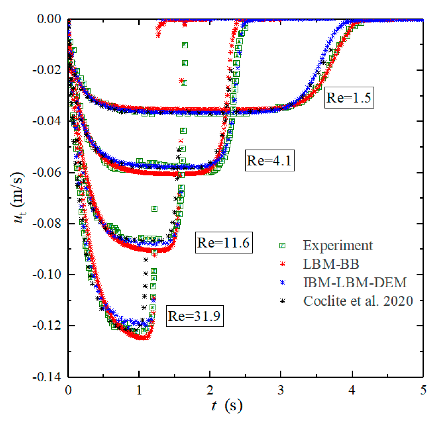
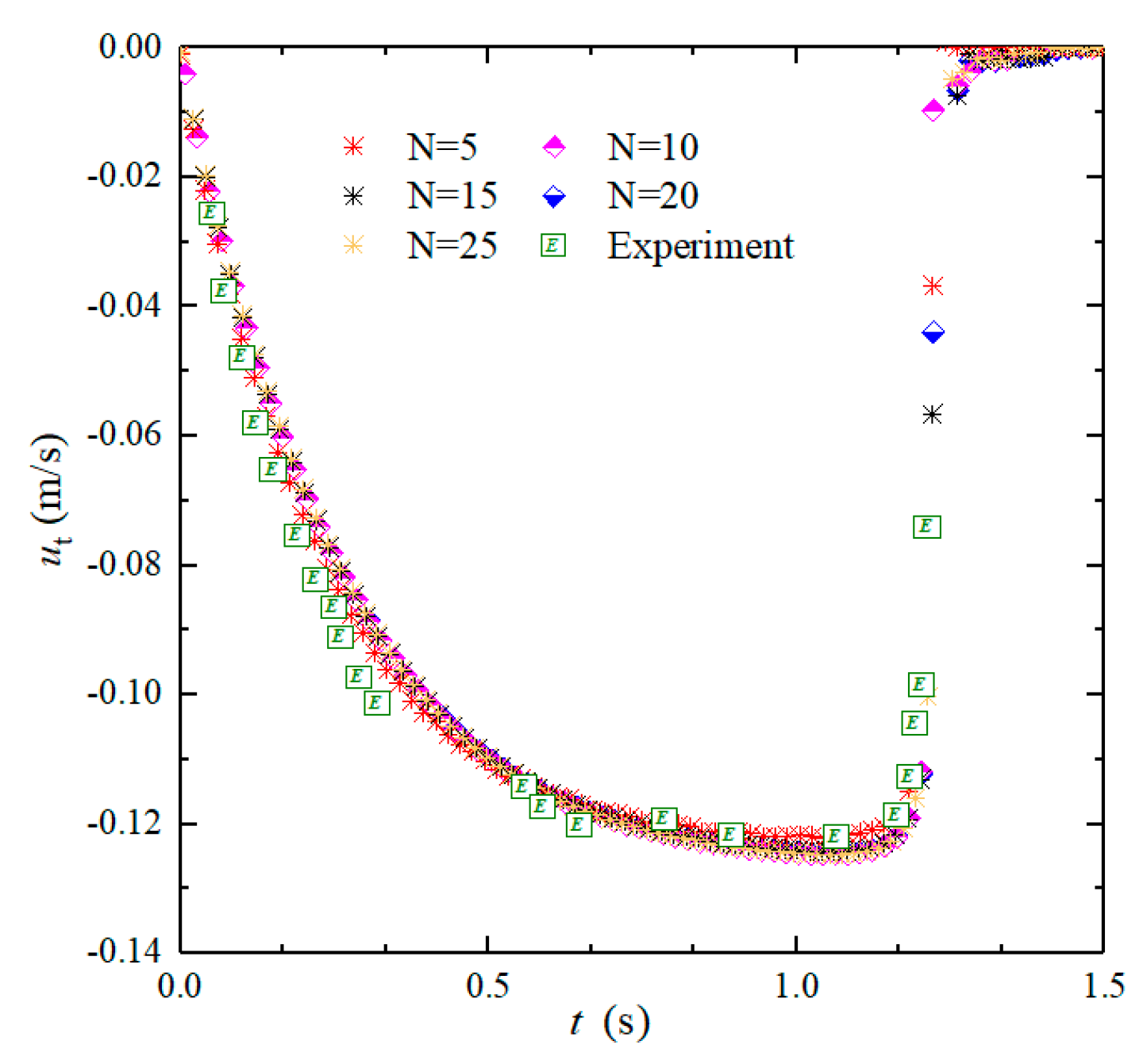
3.1. Single-Particle Sedimentation

The experiment of Cate et al. (2002) [34] as shown in

Table 1. Setup of single-particle sedimentation experiments.

Case Number	${\mathit{\rho }}_{\mathit{f}}$ (kg/m³)	${\mathit{\mu }}_{\mathit{f}}$ (Ns/m²)	${\mathit{u}}_{\mathit{\infty }}$ (m/s)	Re	St
Case 1	970	373	0.038	1.5	0.19
Case 2	965	212	0.060	4.1	0.53
Case 3	962	113	0.091	11.6	1.50
Case 4	960	58	0.128	31.9	4.13

was set up by placing a small sphere of 0.015 m in diameter at a height of 0.12 m in the center of a container, the size of which is 0.1 m × 0.1 m × 0.16 m. The sphere was let to freely settle with terminal Re of 1.5, 4.1, 11.6, and 31.9. In IBM-LBM-DEM, the simulation was carried out by directly adopting the parameters of the experiment (fluid density, particle density, fluid viscosity, particle terminal Re). In both LBM-BB and IBM-LBM-DEM, the container was resolved by 68 × 68 × 108 grids. The particle was resolved by 10 lattices (resolution) across its diameter. The relaxation time τ of LBM-BB was set to 0.6. The gravity acceleration is −9.8 m/s². In single-particle sedimentation simulations, the boundary conditions of all surfaces are no-slip. In LBM-BB, there was a difference between the hydrodynamic diameter and the geometric diameter. The hydrodynamic correction ∆_H = 0.224 used in this study was established through drag calibration (Ladd and Verberg 2001). Coclite et al. [42] developed a dynamic IB scheme combined with LBGK and employed moving least squares reconstruction to accurately interpolate the flow and force fields required to enforce boundary conditions on immersed geometry. Therefore, the simulation results of Coclite et al. are also included for comparison.

Figure 3 shows velocities as functions of time for the four cases. Experimental data (from Cate et al. [43]) and simulation date from Coclite et al. [42] were also included for comparison. In all simulations, the particle’s velocity increased until gravity, buoyancy, and drag forces reached a balance, after which the settling velocity became constant. As the particle approached the bottom wall, its velocity decreased and eventually became zero. In all simulations, both LBM-BB, IBM-LBM-DEM, and Coclite et al.’s simulation results agree with the experiments. By monitoring the settling velocity over time, different methods have been documented to be in excellent agreement. It can also be proved that the IBM-LBM-DEM method adopted in this paper has the same accuracy as other developed methods. When Re is small, the deviation of settling velocities between IBM-LBM-DEM and the experiment is greater than between the LBM-BB method and the experiment. However, at the three higher Re, the settling velocities by the LBM-BB method became greater than the experimental results, and the settling velocities by the IBM-LBM-DEM method are closer to the experimental results. The higher the particle resolution, the more accurate the calculation of particle motion information, but the larger the number of grids at the same time. A grid effect on numerical results is obtained for the IBM-LBM-DEM method to choose an accurate and appropriate resolution. We increased the lattice resolution of the particle from 5 to 25 and re-simulated the case with Re = 31.9. Figure 4 shows that under the simulation result the resolution is 5, and the sedimentation velocity is a little smaller than others. Resolutions ranging from 10 to 25 have little effect on the simulation results with a particle Reynolds number of 31.9. It can be considered that the resolution of 10 is suitable for Re = 31.9. To improve the accuracy at higher Re (>31.9), however, in the next section we doubled the resolution to 20.

3.2. Two-Particle Sedimentation

In two-particle sedimentation, when the initial positions of the two particles are in-line with gravity, the upper particle will catch up with the lower particle. After a collision, the pair turns horizontal and separates. This process is called drafting-kissing-tumbling, DKT. In this section, we used IBM-LBM-DEM to simulate DKT.

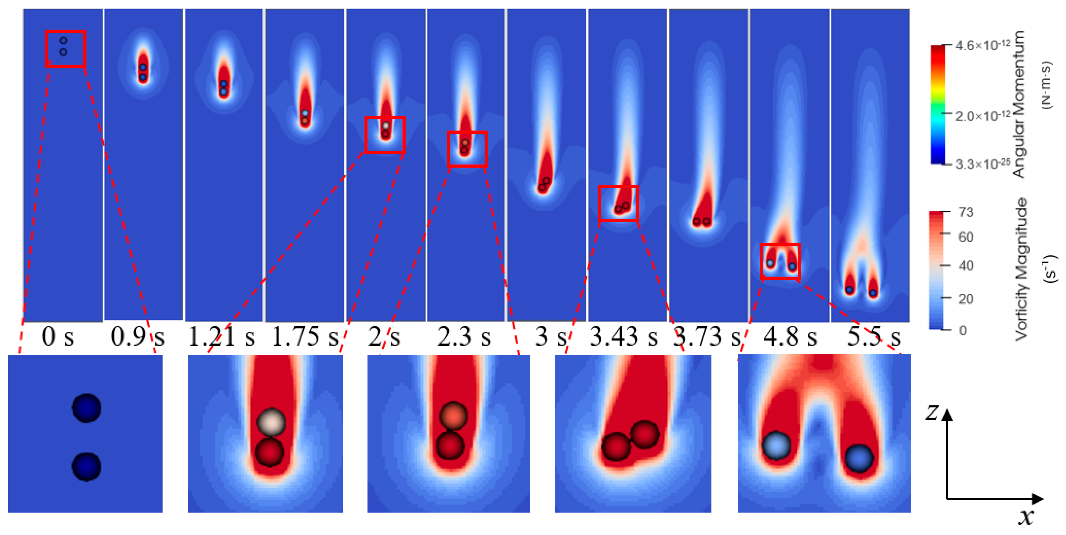
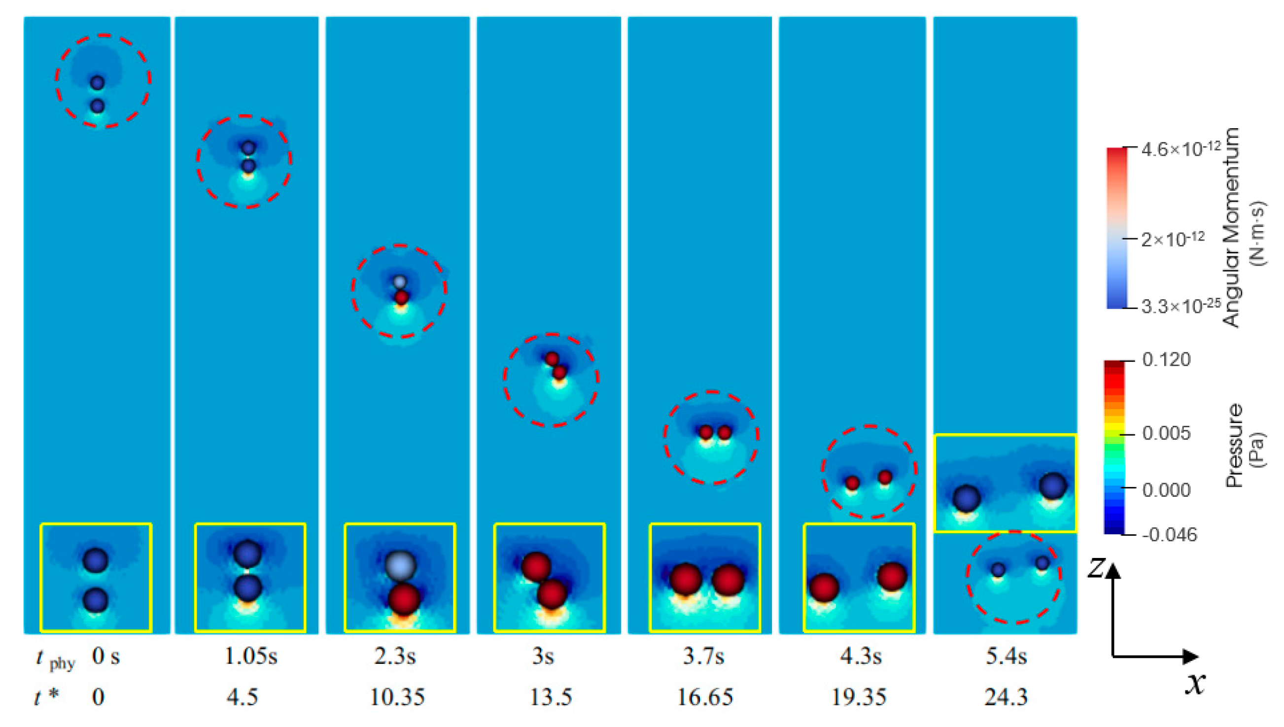
3.2.1. Simulation of DKT

Two particles were placed in a domain 0.02 m × 0.02 m × 0.08 m in size. The diameter of both particles is 0.002 m. The diameter of a single particle is resolved by 10 grids when Re ≤ 31.9 and 20 grids when Re > 31.9. The upper particle is named particle 1 and the lower particle is named particle 2. These two particles were released from position (0.01, 0.01, 0.072) and position (0.0099, 0.01, 0.069). A small offset in the x-positions of the particles was set to enhance the instability of the pair so that they can exercise DKT. In the simulation, the following boundary conditions are used for the computational domain. For the z-direction (settlement direction), the bottom wall is a non-slip wall, and both the x-direction and the y-direction (horizontal direction) are periodic boundaries.

Figure 5 exhibits the distributions of vorticity (magnitude) around the two in-tandem particles, the terminal Re of which is 18.18, at several typical moments in the sedimentation process. The particles are colored based on their angular momenta (magnitude). Particle 1 is drafted by the wake of particle 2 and falls onto particle 2. The nearly in-line configuration of the two particles, however, is not stable. The two particles hence begin to rotate. After particle 1 moves from on top of particle 2 to the side of particle 2, they separate in the horizontal direction due to the opposite signs of their shed y-vorticity.

Figure 6 shows the velocities of the two particles in series in the x and z directions. Particle settling time is nondimensionalized as $t^{*}=t_{phy}/\left(D_p/u_t\right)$, and the dimensionless velocities are velocities normalized by the terminal velocity of the particles. The falling process of particles goes through three stages: drafting-kissing-tumbling, and the pressure also changes in the whole process. This change leads to the interaction of attraction and repulsion of particles, which is consistent with Bernoulli’s law of inviscid fluid. In the initial period of t* < 2, the accelerations of the two particles suggest that they did not “feel” each other hydrodynamically. As settling continued, as Figure 7 shows, a zone of positive pressure was created on the foreside of particle 2, and a zone of negative pressure was created on the aft side. Since particle 1 is in the negative pressure zone of particle 2, the drag force acting on particle 1 is reduced, causing particle 1 to accelerate relative to particle 2. The distance between two particles gradually approaches, and the fluid between particles is “extruded”. Therefore, at this time, the fluid pressure is transformed into kinetic energy, which further causes the rise of fluid velocity between particles and the proximity of two particles, that is, particle attraction. After particle 1 caught up with particle 2 and collided, they settled together for a short period (5.5 < t* < 7). The asymmetry of the vorticity structure around the pair caused the pair to rotate. The foreside of particle 1 became exposed to the incoming flow (3 s, or, t* = 13.5), and a high-pressure zone began to develop on the foreside of particle 1. This high-pressure zone gradually separated particles 1 and 2. Figure 6 suggests that the particles began to develop different x-velocities with separation and the settling velocities of both particles decreased. After particles 1 and 2 completely separated, their shed vorticities had no interactions with each other and they again reached identical settling velocities (22 < t* < 26).

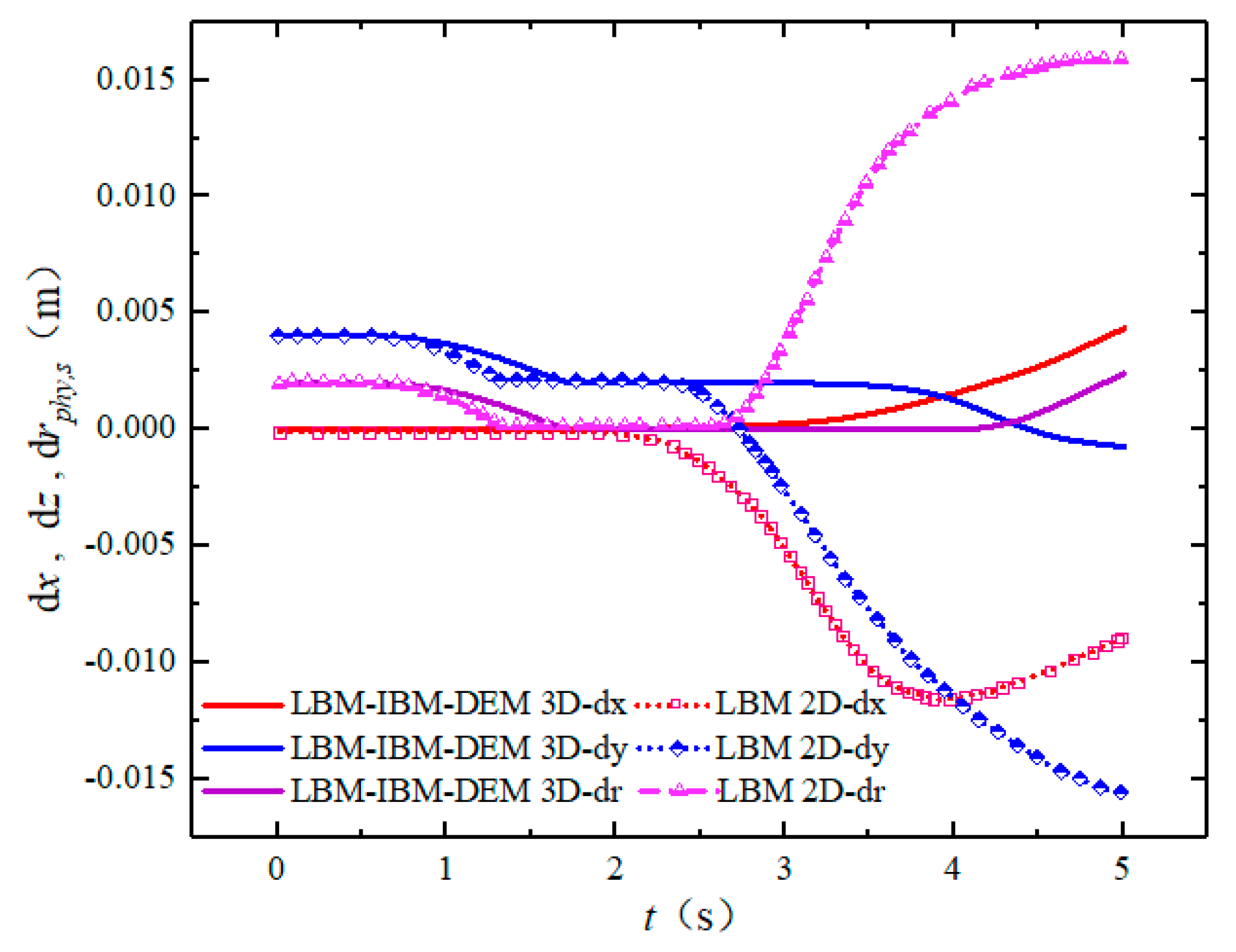
3.2.2. Comparison of 2D and 3D DKT

In this section, we compare the evolutions in the distance between two particles from 2D and 3D DKT. Here, dx, dy, and dz represent the x-, y-, and z-distance between the particles, respectively. dr is the surface-to-surface distance and is defined as $\mathrm{d}{r}_{phy,s}=\sqrt{\mathit{d}{x}^2+\mathit{d}{y}^2+\mathit{d}{z}^2}-D_{\mathrm{p}}$. The distances dx, dz, and dr as functions of time from IBM-LBM-DEM and the 2D DKT of Wang et al. [10] are presented in Figure 8. In our simulation, since we only offset particles’ positions in x but not in y, dy is very small. Hence, dy is not included in Figure 8. The surface-to-surface x-distance between particle 1 and particle 2 decreased before the collision, as expected. Consistent with the conclusions obtained by Nie et al. [15], the dynamics of particles in 2D simulations and that in 3D simulations are different. The most striking difference in the character of DKT, however, is that after tumbling 2D particles separated significantly more than 3D particles. The reason for this difference is that the hydrodynamic interaction between particles decreases with increasing separation much slower in 2D than in 3D.

4. The Effect of Particle relative Position and Rep on DKT

The dynamics of DKT are not only related to the particle Reynolds number that determines the intensity and the distribution of shed vorticity, but also to the initial relative positions (including angles and distances) of the two particles. In this section, we present a systematic study on the effect of particle relative position and Re on DKT.

Table 2. Summary of simulation parameters exploring the effect of relative position and particle Re on DKT.

Parameter	Value
particle centroid distance	1.5 Dp, 2.0 Dp, 3.0 Dp, 4 Dp
initial angle, °	0, 15, 30, 45, 60 and 90
Re	1.82, 18.18, 180.18

shows the parameters studied. In all, we simulated 72 conditions of different Re, angles, and relative distances. We changed Re by changing the viscosity of the fluid, which means that the relax time is the variable parameter for a different case. Particle–fluid density ratio was not changed in the simulations, and dimension properties of fluid and particles and computational domain size are the same as those in 3.2.1. Particle surface-to-surface distance is presented non-dimensionally as $\mathrm{d}{r}_s*=\left(\mathrm{d}{r}_{\mathrm{phy}}-D_p\right)/D_p$. Particle center-to-center distance is presented non-dimensionally as $\mathrm{d}r*=\mathrm{d}{r}_{\mathrm{phy}}/D_p$. The horizontal force that arises from particle–particle interaction is presented non-dimensionally as $f_x^{*}=f_x{}_{,phy}/\left(m_{p}g\right)$, where $m_{p}g$ is particle’s gravity force. Lastly, the non-dimensional angular velocity is ${\omega }^{*}={\omega }_{phy}D/\left(2u_t\right)$. Figure 9 displays the relative positions that were studied.

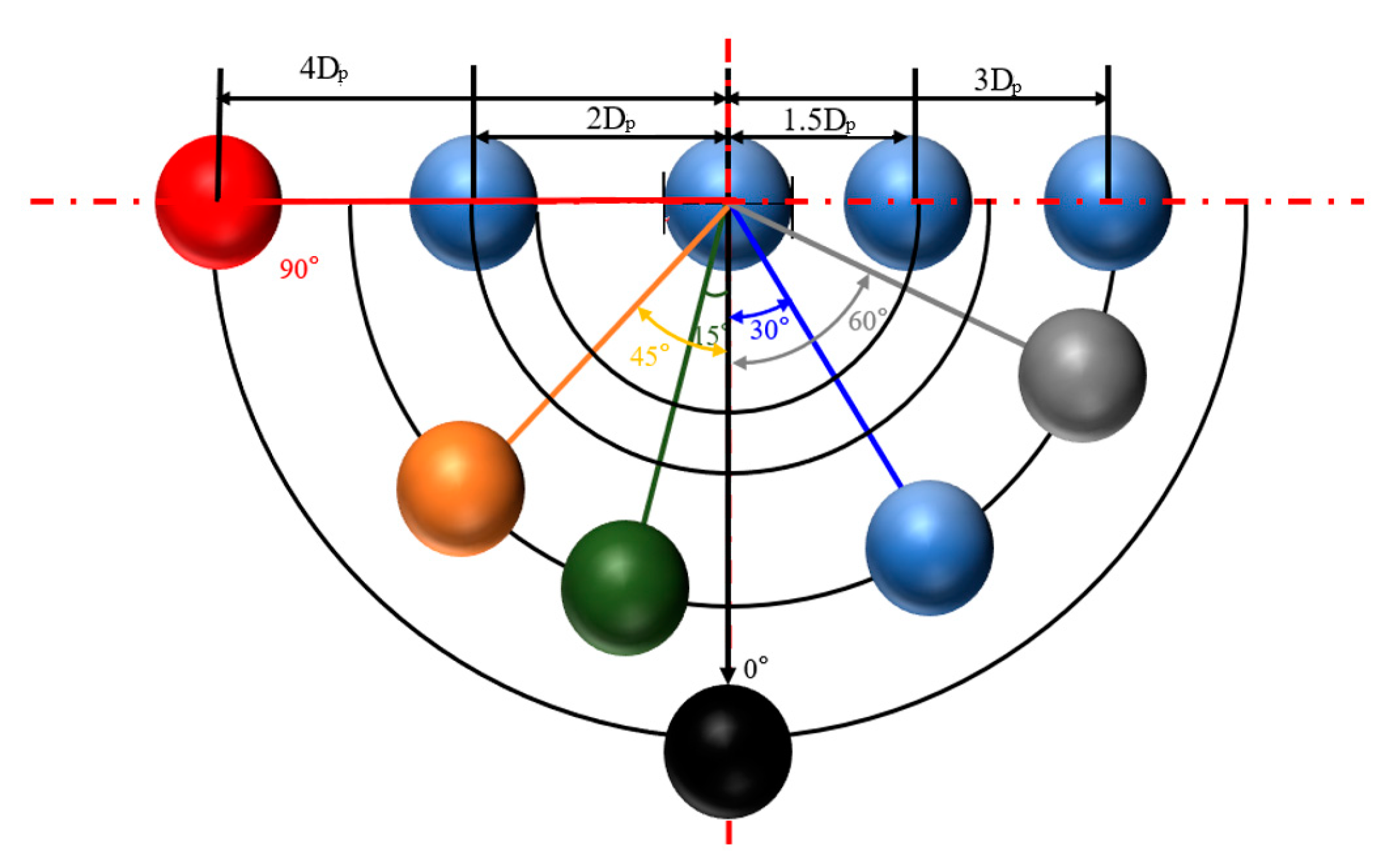
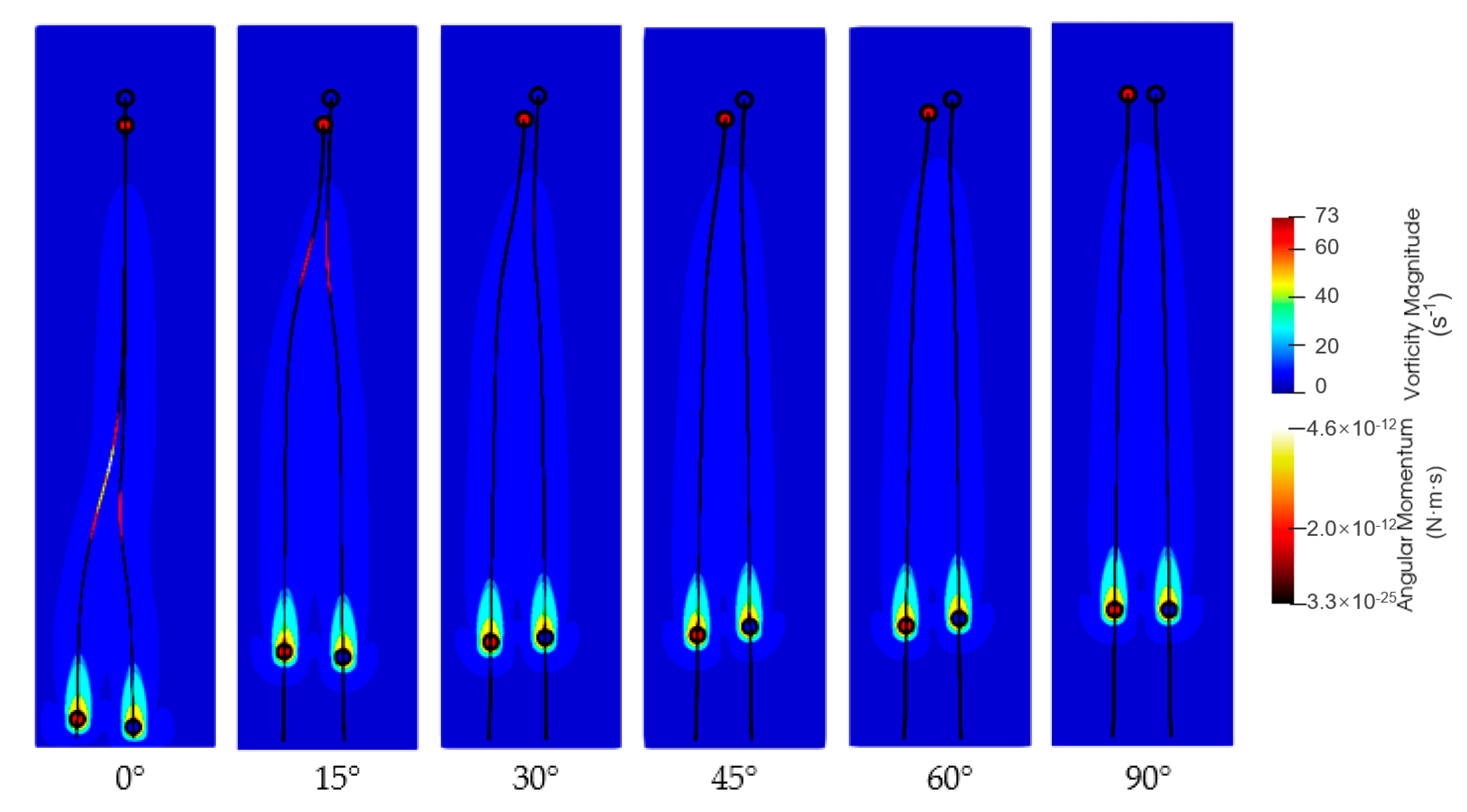
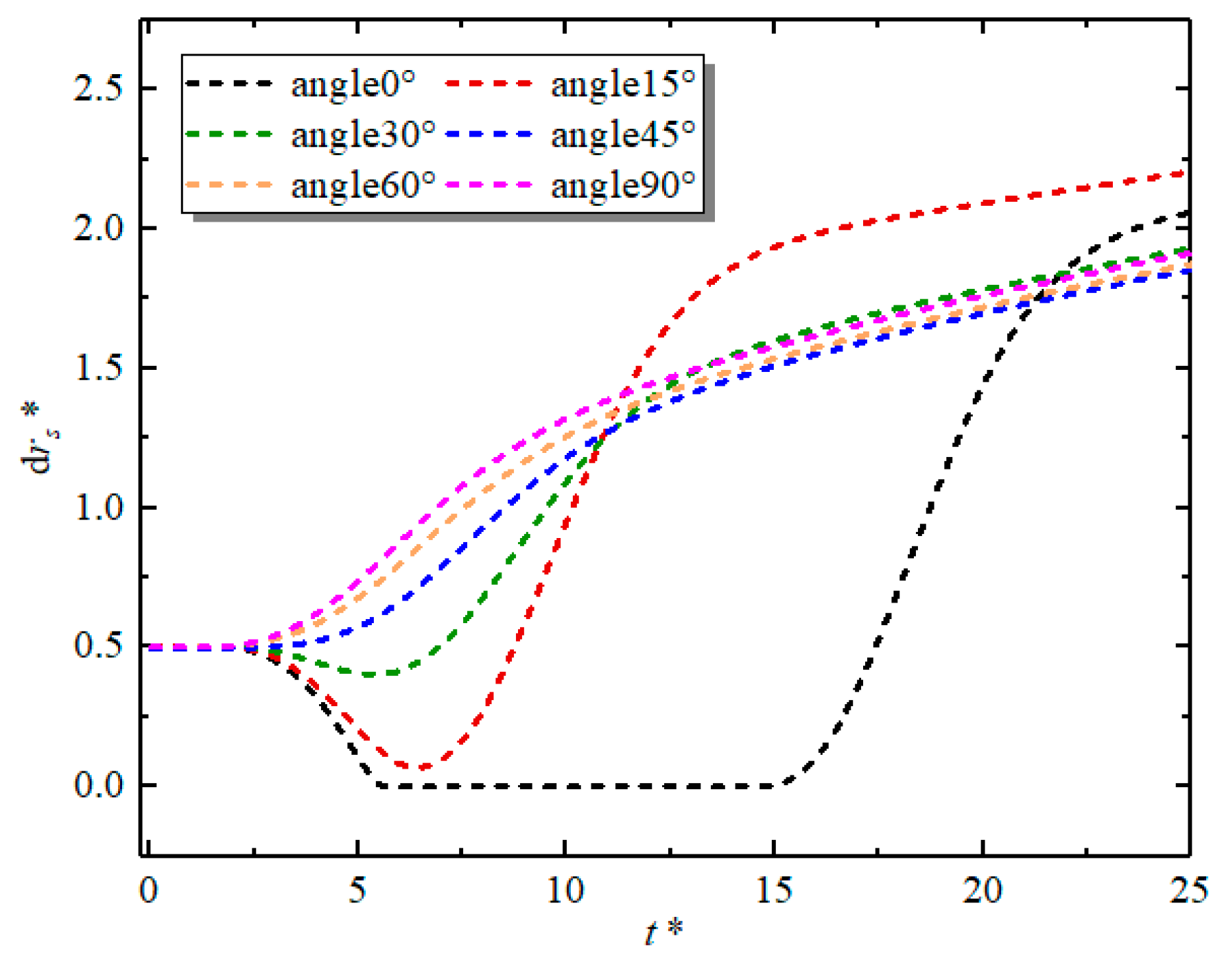
4.1. The Effect of Particle Relative Position

Figure 10 shows the vorticity fields at 6 s and particles’ trajectories. The color of the trajectories represents the magnitude of angular momenta of the particles. Both separation and Re are constant in Figure 10. Hence, the effect of angle is examined. At the angle of 0°, DKT took place but “tumbling” was slow, leading to late lateral separation. At 15°, after a short period of free settling, DKT was triggered. In this DKT, particle 1 was rapidly turned to the side of particle 2. The angular momenta of both particles increased. The two particles then repelled each other and separated. The two particles did not get very close to each other and the angular momenta of the particles were always low. Both the maxima of the angular momenta and the times of their occurrences decreased with increasing initial angle. As particle 2 is no longer in particle 1′s wake, the attraction between the two particles diminished at higher angles. Instead, repulsion between the particles developed. The greater the angle, the stronger the repulsive force. This repulsive force separated the particles horizontally. As the horizontal distance between the two particles increases, the strength of the repulsive force decreases. In the end, the particles settled side-by-side without significant interaction. Kim et al. [8] studied the pressure distribution of two particles in static parallel and found a pressure difference between the pressures on both sides of the particles. The repulsive force between two moving particles is also for the same reason. The pressure of the flow field in the moving particle interval is greater than the pressure outside the particles, and the particles will repel each other under the push of this pressure difference.

If the two particles are treated as a single entity, this entity achieves the highest settling velocity when it is in line with the direction of gravity (the angle of the particles is 0°). However, DKT always increases the angle of the pair toward 90° and hence decreases the average settling velocity of the pair. In dilute suspensions with moderate Re, Yin and Koch [44] found that the average settling velocity rapidly decreased from the terminal velocity with increasing solid fraction. They attributed that rapid decrease to DKT. Conversely, if the relative angle of the particles could be managed to be more in line with gravity in dilute and moderate Re suspensions, DKT could be used to accelerate particle sedimentation.

Figure 11 shows the dimensionless surface-to-surface distance of particles as functions of time. When the angle is 0°, a clear DKT took place. When the angle is 15°, the particles did not actually touch, however, clear drafting and separation due to tumbling can be noticed in the figure. One may hence infer 15° as an approximate boundary of DKT for Re = 18.18 and the initial separation of 1.5 D_p. When the angle is 30°, although weak drafting was present, the two particles never got very close to each other. DKT hence did not occur. Figure 12 shows the maxima of the dimensionless horizontal force that occurred during sedimentation and the dimensionless times that the maxima occurred. The crossover of f_x1 and f_x2 between 15° and 30° indicates that the dominant force interaction between the two particles changed from attractive in DKT to repulsive when the two particles’ initial conditions became more side-by-side.

First-order and second-order derivatives of surface-to-surface distance to time as functions of time are depicted in Figure 13 and Figure 14. The sign of the first-order derivative, negative or positive, is indicative of whether the two particles are approaching each other or separating. Attraction and repulsion can be characterized by the second-order derivative of the surface-to-surface distance of particles to time. When the second-order derivative is positive, the interaction between particles is repulsive. On the contrary, if the second-order derivative is negative, the interaction force between particles is attractive.

As can be seen from Figure 14, when the initial angle is 0° to 30°, the force between particles was initially attractive but became repulsive after the particles turned side-by-side. We note that in the data for 0°, the first very high positive second-order derivative of short duration is the result of particle–particle contact and is not due to hydrodynamics. When the initial angle is between 45° and 90°, repulsive force dominates throughout the interaction. The dynamics of particles released at 0° shows a strong drafting (negative force), a clear kissing (collision), and a strong repulsion after tumbling. That at 15° does not have a collision but still exhibits strong drafting and repulsion after tumbling. They therefore support our previous statement based on Figure 11—that particles released at 0° and 15° executed DKT. The second-order derivative plot, however, shows that the characteristics of the dynamics at 30° is not qualitatively different from that at 15°. Hence, if we focus on the characteristics of the second-order derivative and relax on the definition of kissing, the dynamics of 30° could also be counted as a DKT.

However, the plot of the magnitude of angular velocities, Figure 15, suggests that the dynamics of 30° lacks sufficient rotation (tumbling) and hence should not be counted as DKT. In Figure 15, the magnitudes of the angular velocities of particles are plotted as functions of time. The maxima of angular velocity decreased with increasing angle. For both particles, the maxima of 0° and 15° stand out. The angular velocities of other initial angles are all significantly lower. For particle 1, both the maximum value and the time of maximum decreased with increasing initial angle. Increasing the angle at constant separation, therefore, made the disturbance to the leading particle occur more readily but with less intensity. For particle 2, except for 90°, at higher angles (30°, 45°, and 60°) the angular velocities of particle 2 are much smaller. Figure 15 shows that the upper particle rotated much less than the lower particle in high-angle interactions. Hence, if we require particles to roll together in the “tumbling” phase, the dynamics at 30° is disqualified.

The contour map of dimensionless minimum separation for different angles and initial distance is displayed in Figure 16. The dimensionless particle–particle minimum separation is defined as representing the minimum distance between particles during sedimentation. When s = 0, particles must have experienced collision. When 0 < s < 1, particles have been pulled closer than their initial distance during sedimentation. Note that the minimum in s cannot be greater than the initial s. Hence, s cannot be greater than one. The variation of s hence is an indication of the intensity of attractive hydrodynamic interaction and whether such attractive hydrodynamic interaction led to a collision. For particles with small initial angles (<10°), s is very close to 0 regardless of separation. It is an indication that for particles that are vertically aligned, DKT can always bring them together. For particles with larger initial angles, attraction weakens. Interestingly, dimensionless minimum separation first decreases and then increases with increasing initial surface-to-surface distance at some intermediate angles. This shows the complexity in which the shed vorticities from the two particles interact with each other during sedimentation.

4.2. The Effect of Reynolds Number

Reynolds number affects the degree of vorticity shedding and the fore-aft symmetry of flow around the particle. The dynamics of particle pair settling and DKT are hence a function of Re.

Figure 17 shows the trajectories of particles at two different Reynolds numbers. The initial center-to-center distance is 3 D_p. In Section 4.1, we presented that at small initial angles, particles collide, rotate, and then separate and settle independently following DKT dynamics. At greater initial angles, the leading particle is pushed to the side and then overtaken by the trailing particle. After the relative positions of the two particles switch, the original leading but now trailing particle experiences an attraction (c.f. Figure 14). The two particles can therefore approach each other again and execute another switch in their leading/trailing positions. When the Reynolds number of particles is 18.18, particles’ trajectories crossed only once at 0°, 15°, and 30°. When the particle angle is 45°, particles’ trajectories crossed twice, which means that the leading/trailing positions of the particles switched again before they settled to the bottom of the domain. When Re of particles increased to about 180, DKT only occurred at 0°. Increased Reynolds number leads to decreased influence of fluid viscosity compared to that of particle/fluid inertia, which, in turn, makes the changes in particles’ trajectories less pronounced.

Figure 18 shows the dimensionless particle–particle minimum separation at various initial distance and angles and different Reynolds numbers. It is observed that two particles will collide at an initial angle of 0°, but not at an initial angle of 90°, in the focused range of Re. The surface of s gradually transitions from steep in low-angle region to less steep in low-angle region from small Re to large Re, and the range of initial angle and particles’ distance for attraction increases with increasing Re. The domain of attraction (s < 1) is limited to initial angles less than 55° for small Re of 1.82. When Re is 18.18, some limited attraction can be noticed at short distances and high angles. Figure 18a,b shows that at the two lower Reynolds numbers, the minimum distance increases with the increase of the initial distance. Figure 18a shows that for pairs with short initial distances, the minimum separation distance varies significantly, with initial angle in the range of 20° and 55°. For pairs with longer initial distances, the minimum separation distance varies greatly with initial angle in the range of 10° to 35°. The domain attraction is independent of initial distances when the initial angle in the range of 0° to 30° and the Re of 18.18 as shown in Figure 18b. When Re is raised to 181.8, it is observed that the domain of attraction is significantly expanded. The most striking and qualitative difference, however, is that particle pairs with initial angles in the range of 40–70° showed strong attractions at high separations, shown in Figure 18c, likely due to inviscid potential flow interactions that dominate the interactions between pairs of high-Re and spherical gas bubbles, but nonetheless should also exist between high-Re solid particles when their viscous boundary layers do not overlap [45,46,47].

5. Conclusions

The present work employs an IBM-LBM-DEM method to analyze the settling of two particles with hydrodynamic interactions. Our method was verified by comparing single-particle settling velocities to those measured in experiments. Our main observations from two-particle simulations are as follows:

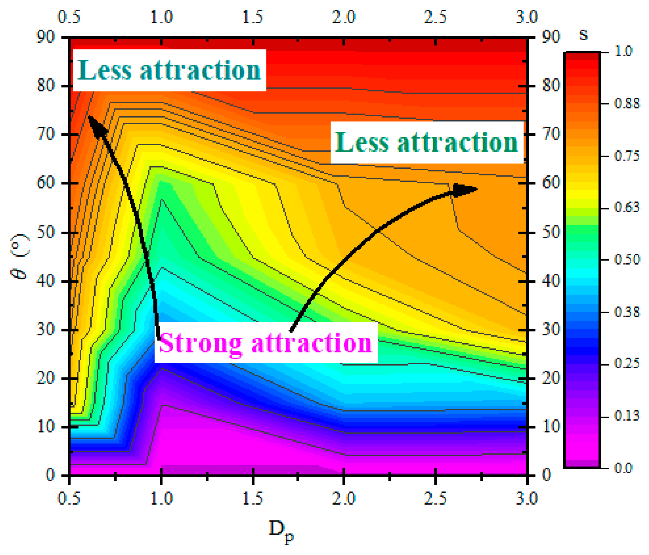
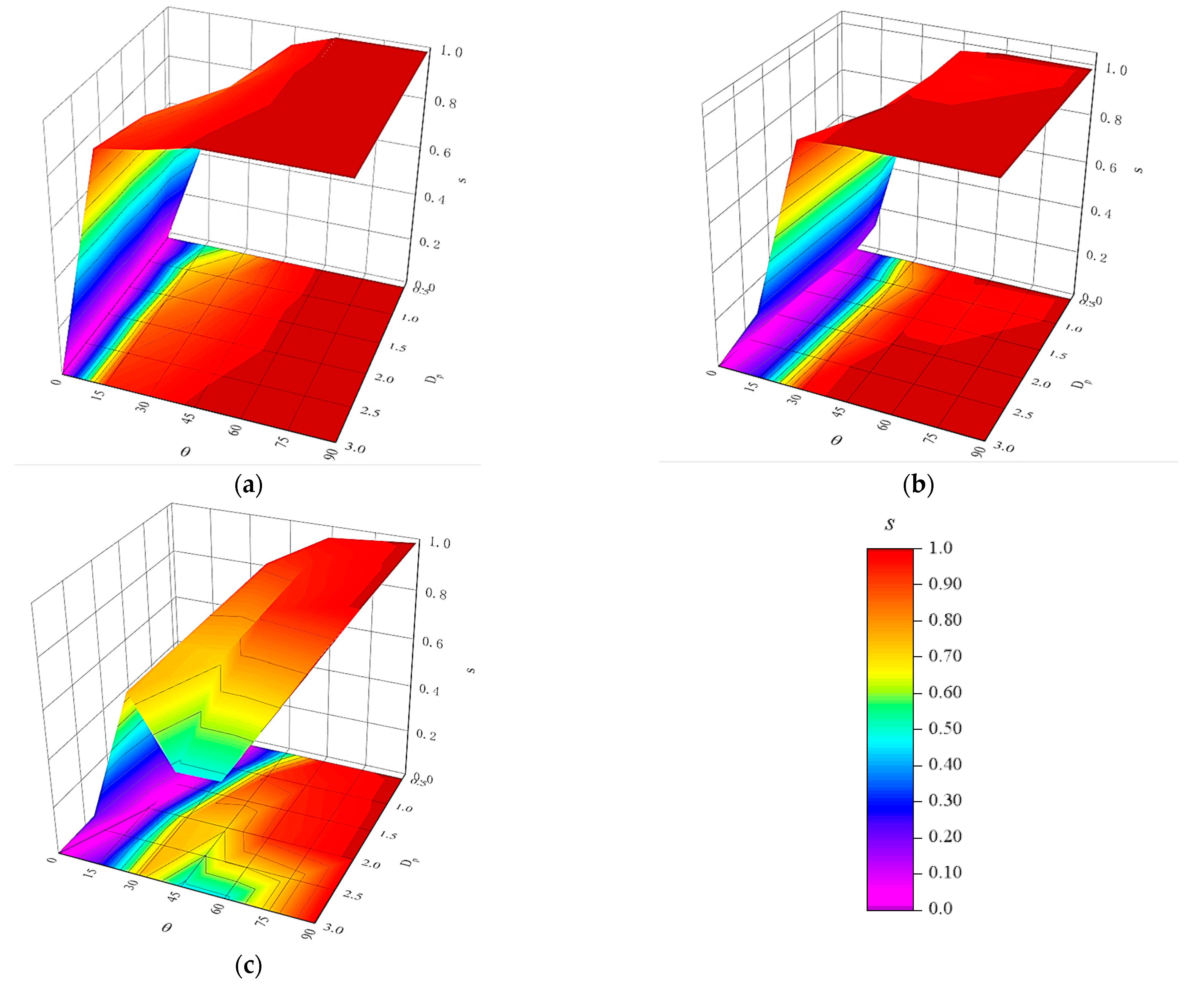
• Whether the hydrodynamic interaction between particles is attractive or repulsive during sedimentation depends on the relative location of the particles and the Reynolds number.
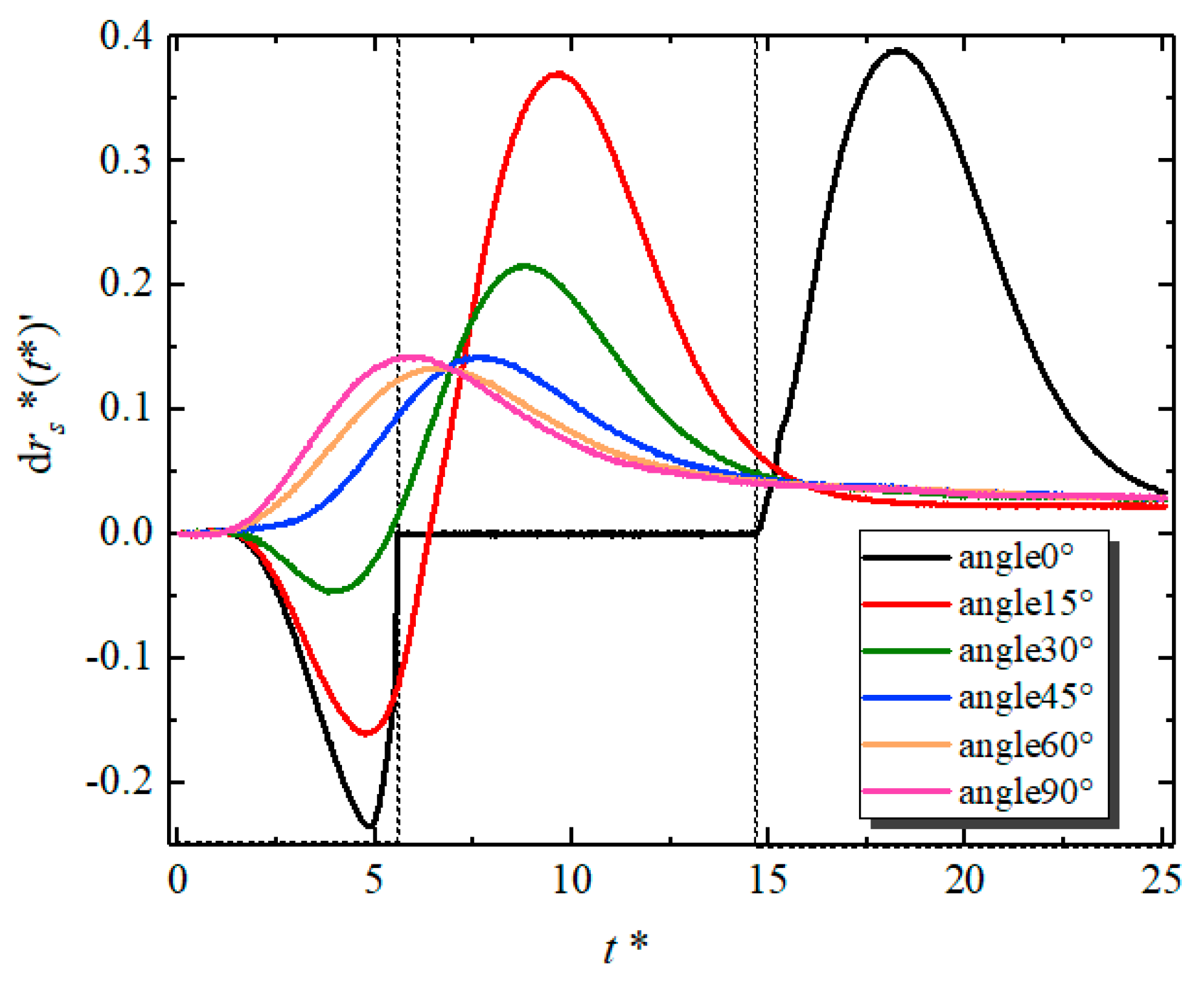
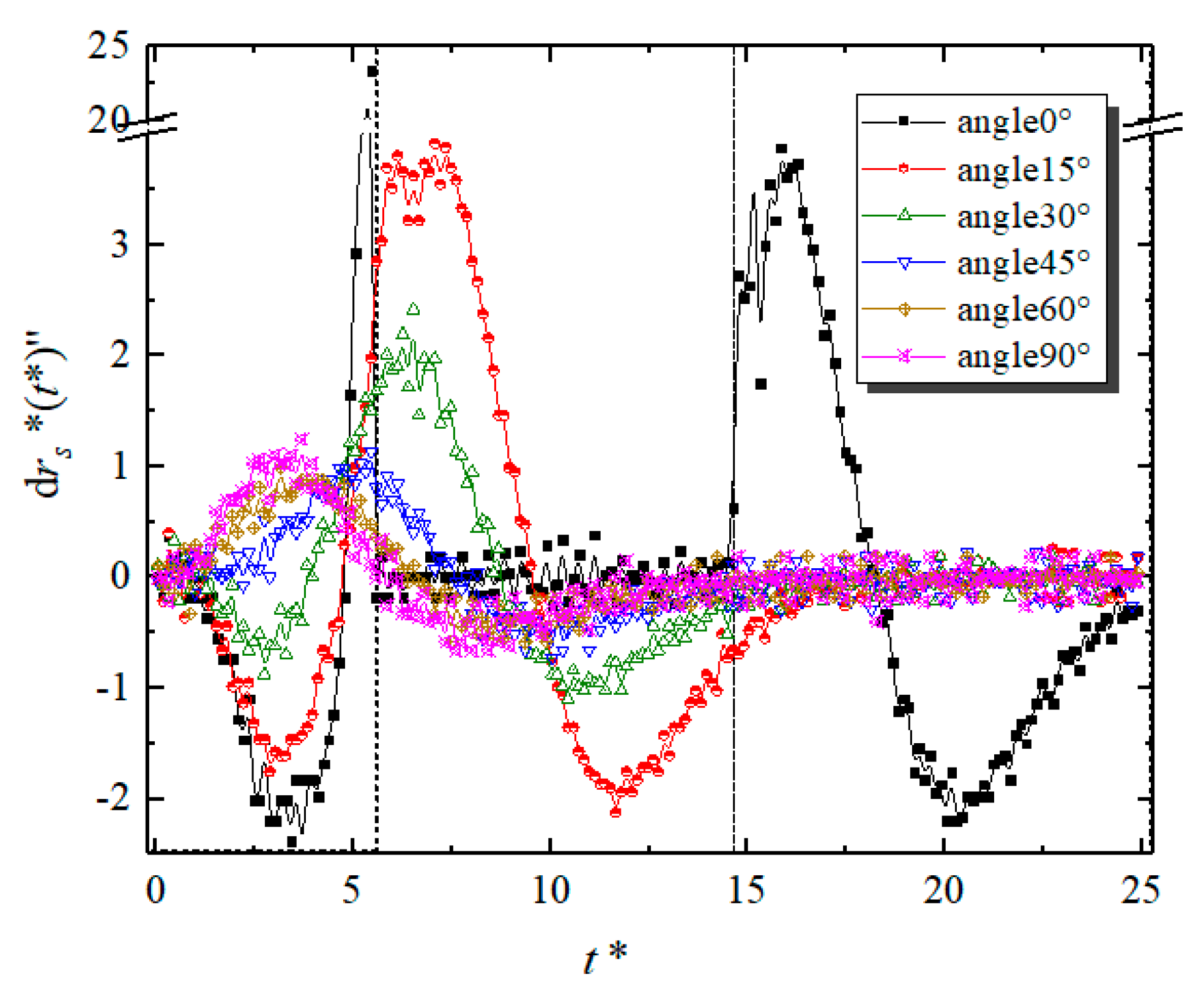
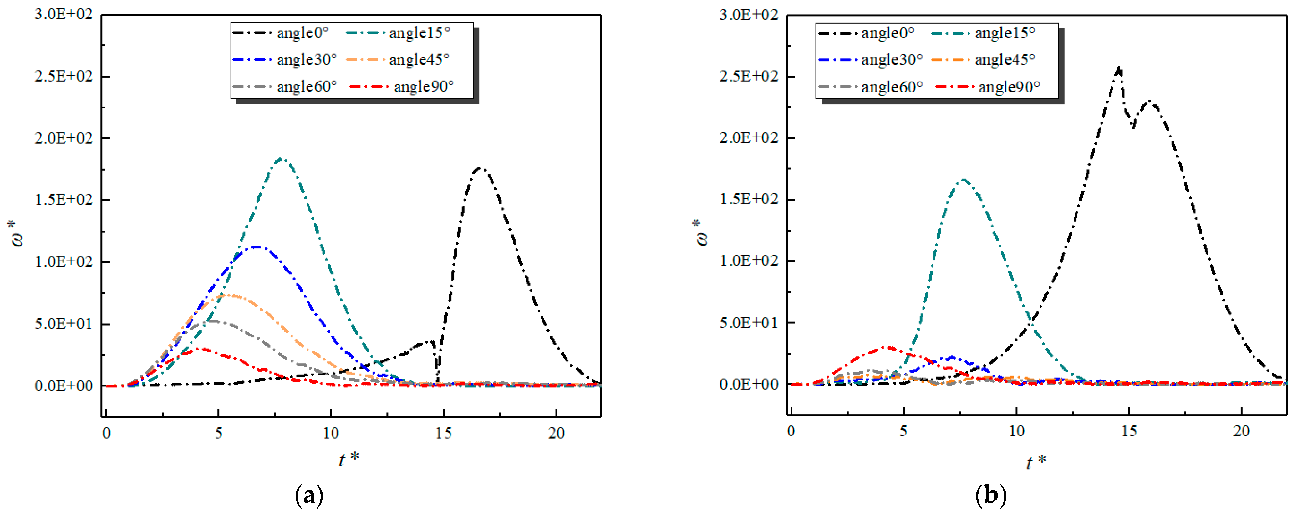
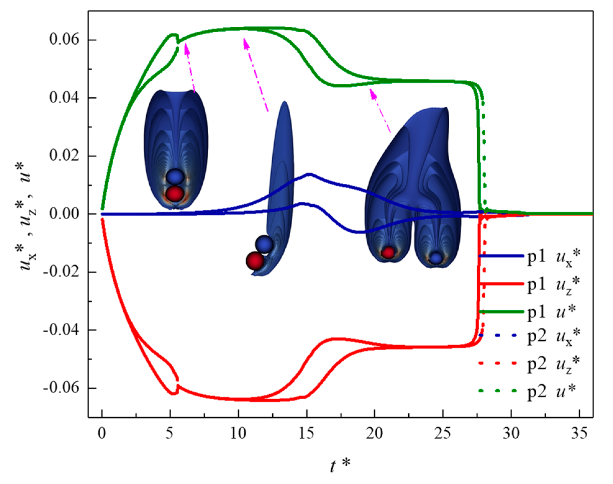
• Whether a pair of particles has experienced DKT can be viewed from time plots of the distance between the particles (for kissing), the second-order derivative of distance to time (for drafting), and angular velocities of particles (for tumbling). In a DKT, particles should approach each other along the vertical direction to a close distance, develop nearly equal and opposite angular velocities, and then separate along the horizontal direction.
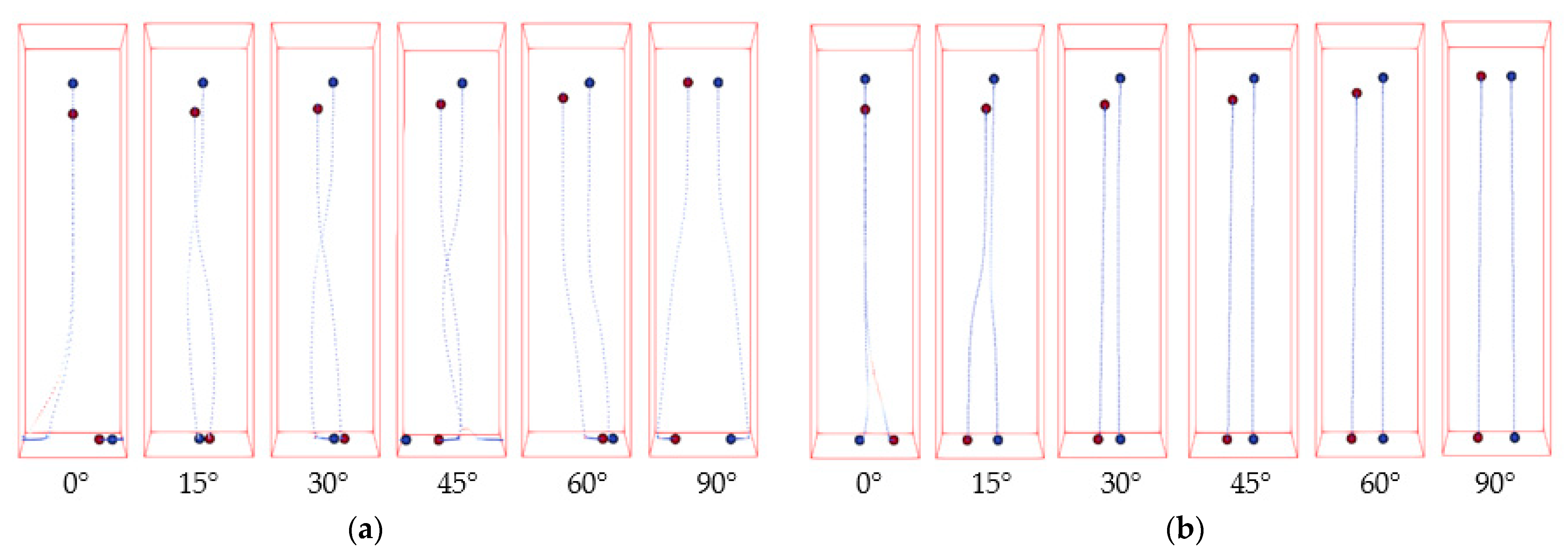
• As expected, not all combinations of initial distance, angle, and Reynolds number lead to DKT. DKT only occurs when the initial positions of particles are nearly vertically aligned. At high Reynolds numbers, due to high particle/fluid inertia, the influence of fluid–particle force on particles’ trajectories becomes less. Particles hence could generally get closer to each other at higher Reynolds numbers, regardless of whether the interaction is DKT or not.
• When Re is low or moderate (O(1–10)), particle pairs with high initial angles do not experience attraction. When Re is high (O(100)), however, our results show that the domain of attractive interaction significantly expanded and particle pairs with initial angles in the range of 40–70° also experienced attraction at long initial distances (2.5 to 3.0 D_p) likely attributed to inviscid potential flow interaction.
• The IBM-LBM-DEM method is consistent with other numerical simulation results and experimental data. Collectively, the proposed approach can be efficiently used for predicting complex particle dynamics relevant flows.

References

- Di, Y.; Zhao, L.; Mao, J. A resolved CFD-DEM method based on the IBM for sedimentation of dense fluid-particle flows. Comput. Fluids 2021, 226, 104968. [Google Scholar] [CrossRef]
- Kim, I.; Elghobashi, S.; Sirignano, W.A. Three-dimensional flow over two spheres placed side by side. J. Fluid Mech. 1993, 246, 465–488. [Google Scholar] [CrossRef]
- Mccullough, J.; Leonardi, C.R.; Jones, B.D.; Aminossadati, S.M.; Williams, J.R. Lattice Boltzmann methods for the simulation of heat transfer in particle suspensions. Int. J. Heat Fluid Flow 2016, 62, 150–165. [Google Scholar] [CrossRef]
- Fortes, A.F.; Joseph, D.D.; Lundgren, T.S. Nonlinear mechanics of fluidization of beds of spherical particles. J. Fluid Mech. 1987, 177, 467–483. [Google Scholar] [CrossRef]
- Feng, J.; Hu, H.H.; Joseph, D.D. Direct simulation of initial value problems for the motion of solid bodies in a Newtonian fluid Part 1. Sedimentation. J. Fluid Mech. 1994, 261, 95–134. [Google Scholar] [CrossRef] [Green Version]
- Patankar, N.A.; Singh, P.; Joseph, D.D.; Glowinski, R.; Pan, T.W. A new formulation of the distributed Lagrange multiplier/fictitious domain method for particulate flows. Int. J. Multiph. Flow 2000, 26, 1509–1524. [Google Scholar] [CrossRef]
- Niu, X.D.; Shu, C.; Chew, Y.T.; Peng, Y. A momentum exchange-based immersed boundary-lattice Boltzmann method for simulating incompressible viscous flows. Phys. Lett. A 2006, 354, 173–182. [Google Scholar] [CrossRef]
- Feng, Z.G.; Michaelides, E.E. The immersed boundary-lattice Boltzmann method for solving fluid–particles interaction problems. J. Comput. Phys. 2004, 195, 602–628. [Google Scholar] [CrossRef]
- Jafari, S.; Yamamoto, R.; Rahnama, M. Lattice-Boltzmann method combined with smoothed-profile method for particulate suspensions. Phys. Rev. E Stat. Nonlinear Soft Matter Phys. 2011, 83, 026702. [Google Scholar] [CrossRef]
- Wang, L.; Guo, Z.L.; Mi, J.C. Drafting, kissing and tumbling process of two particles with different sizes. Comput. Fluids 2014, 96, 20–34. [Google Scholar] [CrossRef]
- Ladd, A.; Verberg, R. Lattice-Boltzmann Simulations of Particle-Fluid Suspensions. J. Stat. Phys. 2001, 104, 1191–1251. [Google Scholar] [CrossRef]
- Hu, Y.; Li, D.; Shu, S.; Niu, X. Modified momentum exchange method for fluid-particle interactions in the lattice Boltzmann method. Phys. Rev. E Stat. Nonlinear Soft Matter Phys. 2015, 91, 033301. [Google Scholar] [CrossRef] [PubMed]
- Cao, C.; Chen, S.; Li, J.; Liu, Z.; Zha, L.; Bao, S.; Zheng, C. Simulating the interactions of two freely settling spherical particles in Newtonian fluid using lattice-Boltzmann method. Appl. Math. Comput. 2015, 250, 533–551. [Google Scholar] [CrossRef]
- Liu, S.; Zhou, T.; Tao, S.; Wu, Z.; Yang, G. Lattice Boltzmann simulation of particle-laden flows using an improved curved boundary condition. Int. J. Mod. Phys. C 2019, 30, 1950041. [Google Scholar] [CrossRef]
- Nie, D.; Guan, G.; Lin, J. Interaction between two unequal particles at intermediate Reynolds numbers: A pattern of horizontal oscillatory motion. Phys. Rev. E 2021, 103, 013105. [Google Scholar] [CrossRef]
- Dash, S.M.; Lee, T.S. Two spheres sedimentation dynamics in a viscous liquid column. Comput. Fluids 2015, 123, 218–234. [Google Scholar] [CrossRef]
- Liao, C.C.; Hsiao, W.W.; Lin, T.Y.; Lin, C.A. Simulations of two sedimenting-interacting spheres with different sizes and initial configurations using immersed boundary method. Comput. Mech. 2015, 55, 1191–1200. [Google Scholar] [CrossRef]
- Yang, B.; Chen, S.; Xiong, Y.; Zhang, R.; Zheng, C. Size and thermal effects on sedimentation behaviors of two spheres. Int. J. Heat Mass Transf. 2017, 114, 198–206. [Google Scholar] [CrossRef] [Green Version]
- Nie, D.; Lin, J. Simulation of sedimentation of two spheres with different densities in a square tube. J. Fluid Mech. 2020, 896, 1–27. [Google Scholar] [CrossRef]
- Tao, S.; Guo, Z.; Wang, L. Numerical study on the sedimentation of single and multiple slippery particles in a Newtonian fluid. Powder Technol. Int. J. Sci. Technol. Wet Dry Part. Syst. 2017, 315, 126–138. [Google Scholar] [CrossRef] [Green Version]
- Zhang, J.F.; Maa, P.Y.; Zhang, Q.H.; Shen, X.T. Direct numerical simulations of collision efficiency of cohesive sediments. Estuar. Coast. Shelf Sci. 2016, 178, 92–100. [Google Scholar] [CrossRef]
- Vowinckel, B.; Withers, J.; Luzzatto-Fegiz, P.; Meiburg, E. Settling of cohesive sediment: Particle-resolved simulations. J. Fluid Mech. 2018, 858, 5–44. [Google Scholar] [CrossRef] [Green Version]
- Chen, H.; Liu, W.; Chen, Z.; Zheng, Z. A numerical study on the sedimentation of adhesive particles in viscous fluids using LBM-LES-DEM. Powder Technol. 2021, 391, 461–478. [Google Scholar] [CrossRef]
- Liu, J.; Zhang, P.; Xiao, Y.; Wang, Z.; Yuan, S.; Tang, H. Interaction between dual spherical particles during settling in fluid. Phys. Fluids 2021, 33, 013312. [Google Scholar] [CrossRef]
- Karvelas, E.; Liosis, C.; Theodorakakos, A.; Sarris, I.; Karakasidis, T. An Optimized Method for 3D Magnetic Navigation of Nanoparticles inside Human Arteries. Fluids 2021, 6, 97. [Google Scholar] [CrossRef]
- Lampropoulos, N.K.; Karvelas, E.G.; Sarris, I.E. Computational study of the particles interaction distance under the influence of steady magnetic field. Adv. Syst. Sci. Appl. 2015, 15, 233–241. [Google Scholar]
- Karvelas, E.G.; Lampropoulos, N.K.; Sarris, I.E. A numerical model for aggregations formation and magnetic driving of spherical particles based on OpenFOAM. Comput. Methods Programs Biomed. 2017, 142, 21–30. [Google Scholar] [CrossRef]
- Griffith, B.E.; Patankar, N.A. Immersed Methods for Fluid–Structure Interaction. Annu. Rev. Fluid Mech. 2020, 52, 421–448. [Google Scholar] [CrossRef] [Green Version]
- Peskin, C.S. The immersed boundary method. Acta Numer. 2002, 11, 479–517. [Google Scholar] [CrossRef] [Green Version]
- Chen, S.; Chen, H.; Martnez, D.; Matthaeus, W. Lattice Boltzmann model for simulation of magnetohydrodynamics. Phys. Rev. Lett. 1991, 67, 3776–3779. [Google Scholar] [CrossRef]
- Qian, Y.H.; D’Humieres, D.; Lallermand, P. Lattice BGK models for Navier-Stokes equation. Europhys. Lett. 1992, 17, 479–484. [Google Scholar] [CrossRef]
- Xie, J.; Zhong, W.; Shao, Y. Study on the char combustion in a fluidized bed by CFD-DEM simulations: Influences of fuel properties. Powder Technol. 2021, 394, 20–34. [Google Scholar] [CrossRef]
- Xia, T.; Feng, Q.; Wang, S.; Zhang, J.; Zhang, W.; Zhang, X. Numerical Study and Force Chain Network Analysis of Sand Production Process Using Coupled LBM-DEM. Energies 2022, 15, 1788. [Google Scholar] [CrossRef]
- Han, Y.; Cundall, P.A. Resolution sensitivity of momentum-exchange and immersed boundary methods for solid-fluid interaction in the lattice Boltzmann method. Int. J. Numer. Methods Fluids 2011, 67, 314–327. [Google Scholar] [CrossRef]
- Brilliantov, N.V.; Spahn, F.; Hertzsch, J.M.; Pöschel, T. Model for collisions in granular gases. Phys. Rev. E Stat. Phys. Plasmas. Fluids Relat. Interdiscip. Top. 2002, 53, 5382–5392. [Google Scholar] [CrossRef] [PubMed] [Green Version]
- Coclite, A.; de Tullio, M.D.; Pascazio, G.; Decuzzi, P. A combined Lattice Boltzmann and Immersed Boundary approach for predicting the vascular transport of differently shaped particles. Comput. Fluids 2016, 136, 260–271. [Google Scholar] [CrossRef] [Green Version]
- Coclite, A.; Ranaldo, S.; De Tullio, M.D.; Decuzzi, P.; Pascazio, G. Kinematic and dynamic forcing strategies for predicting the transport of inertial capsules via a combined lattice Boltzmann—Immersed Boundary method. Comput. Fluids 2018, 180, 41–53. [Google Scholar] [CrossRef] [Green Version]
- Coclite, A.; Pascazio, G.; de Tullio, M.D.; Decuzzi, P. Predicting the vascular adhesion of deformable drug carriers in narrow capillaries traversed by blood cells. J. Fluids Struct. 2018, 82, 638–650. [Google Scholar] [CrossRef]
- Noble, D.R.; Torczynski, J.R. A Lattice-Boltzmann Method for Partially Saturated Computational Cells. Int. J. Mod. Phys. C 1998, 9, 1189–1201. [Google Scholar] [CrossRef]
- Seil, P.; Pirker, S. LBDEMcoupling: Open-Source Power for Fluid-Particle Systems. In International Conference on Discrete Element Methods; Springer: Singapore, 2016. [Google Scholar]
- Latt, J.; Malaspinas, O.; Kontaxakis, D.; Parmigiani, A.; Lagrava, D.; Brogi, F.; Belgacem, M.B.; Thorimbert, Y.; Leclaire, S.; Li, S.; et al. Palabos: Parallel Lattice Boltzmann Solver. Applications 2019, 81, 334–350. [Google Scholar] [CrossRef]
- Coclite, A.; Ranaldo, S.; Pascazio, G.; de Tullio, M.D. A Lattice Boltzmann dynamic-Immersed Boundary scheme for the transport of deformable inertial capsules in low-Re flows. Comput. Math. Appl. 2020, 80, 2860–2876. [Google Scholar] [CrossRef]
- Ten Cate, A.; Nieuwstad, C.H.; Derksen, J.J.; Van den Akker, H.E.A. Particle imaging velocimetry experiments and lattice-Boltzmann simulations on a single sphere settling under gravity. Phys. Fluids 2002, 14, 4012–4025. [Google Scholar] [CrossRef]
- Yin, X.; Koch, D.L. Hindered settling velocity and microstructure in suspensions of solid spheres with moderate Reynolds numbers. Phys. Fluids 2007, 19, 093302. [Google Scholar] [CrossRef]
- Biesheuvel, A.; Wijngaarden, L.V. The motion of pairs of gas bubbles in a perfect liquid. J. Eng. Math. 1982, 16, 349–365. [Google Scholar] [CrossRef] [Green Version]
- Kok, J. Dynamics of a pair of gas bubbles moving through liquid. Part I. Theory. Eur. J. Mech. B/Fluids 1993, 12, 515–540. [Google Scholar]
- Kok, J. Dynamics of a pair of gas bubbles moving through liquid. Part II. Experiment. Eur. J. Mech. B/Fluids 1993, 12, 541–560. [Google Scholar]