A Multi-Region CFD Model for Aircraft Ground Deicing by Dispersed Liquid Spray

Abstract

The aircraft ground deicing (AGD) process is a mandatory step before taking off in a cold climate. The development of CFD (computational fluid dynamics) tools to simulate AGD could help the industry reduce its costs and limit pollution. Previous works have modelled some parts of the AGD process. Building on these previous works, this paper presents a three-dimensional (3D) CFD algorithm to simulate the process in full scale. The algorithm comprises a multi-region model where a Lagrangian method solves the spray particle equations, and an enthalpy–porosity approach with an Eulerian method simulates the ice melting. The multi-region approach is verified in this paper through a spray-tip penetration (STP) test. The STP predicted using the multi-region model had 99% agreement with the STP predicted using a Lagrangian method. Therefore, the multi-region technique correctly modeled the particle momentum between the two regions. This paper also presents a numerical calibration of the permeability coefficient for the extended enthalpy–porosity technique in the context of AGD. The numerical calibration of the permeability coefficient will enable future parametric studies of the AGD process.

1. Introduction

Pilots decide to apply ground deicing or anti-icing treatments before take-off on any civil aircraft, if they expect to operate under suspected or known ground ice conditions [1]. Figure 1 presents a scheme of the typical ground deicing process. An operator directs a preheated aircraft deicing fluid (ADF) spray to the contaminated surface. The ice melts and a liquid film, composed of ADF and water, flows over the surface and lands on the tarmac. This operation adds a noticeable cost to flights in winter. Recently, research efforts have focused on improving the deicing process. Process guidelines are suggested in [2,3] based on technical and manufacturer reports, guidance materials and standards, technological patents, and procedures. Most of the guidelines are empirical and not mandatory. However, an audit before take-off guarantees process quality. To improve the process, [4,5] propose a numerical optimization through heat balance analysis. Their model links the ice thickness and the weather with the ADF flow rate and the process time, and offers a potential reduction of up to 20% of consumed ADF volumes.

Figure 1. Representative scheme of the ground deicing process.

A CFD-based test bench of the AGD process could also lead to process improvement. The test bench goal was to study the influence of different parameters, including the spray inclination angle and the flow rate, on the total process time and the required ADF volumes. The test bench involved modeling a dispersed multiphase flow with heat transfer and phase change. To develop the test bench, initial research efforts studied the convective heat transfer between an ADF spray and a surface using the volume-of-fluid (VOF) method [6]. The spray dispersion was omitted in this study. Previous research [7] included replacing the VOF method with a Lagrangian drop in Eulerian fluid (LDEF) method, taking into account the dispersion of the droplets. The model demonstrated a comparable precision of 85% and a lower computation cost.

A previous CFD study [8] was the first to model ice melting with an ADF spray. The study coupled an Eulerian drop in an Eulerian fluid (EDEF) method with an extended version of the enthalpy–porosity technique to simulate the ice melting. Figure 2 presents a typical computational domain for the problem. In the first region, an Eulerian–Lagrangian approach models the multiphase flow of the liquid spray. An EDEF approach models the spray impingement on the ice in the relatively thin second region. Reference [8] validated only the Eulerian region and calibrated the enthalpy–porosity technique in two dimensions. The present work proposes a multi-region model solving simultaneously the two regions and verifies the momentum transfer between the two regions in 3D.

Figure 2. Typical computational domain for the proposed methodology [8].

The EDEF and the LDEF approaches were compared [9]; the authors found similar results for a pipe flow and a separated flow (sudden pipe expansions). Both approaches have their advantages. The LDEF approach is recommended for poly-dispersed distributions. It makes the best prediction for flows with high particle velocity gradients. It reduces particle discretization errors, even if the simulation uses a coarse grid for the fluid phase. These characteristics are associated with the AGD problem and an LDEF approach is favored. Additionally, in the AGD problem, the spray must interact with a liquid film. The addition of a film model to a Lagrangian spray solver requires a dynamic mesh to follow the ice interface. The EDEF approach avoids the need for a dynamic mesh in the ice’s vicinity. The literature review [10] corroborates previous [9] results, adding that the LDEF is superior for mass transfer between phases, such as evaporation.

Another study [11] compared the two approaches for spray simulations, and confirmed the superiority of LDEF for the poly-dispersal feature of the spray topology. The literature review [12] confirmed that LDEF is better than EDEF for poly-dispersed flows and for interphase quantity transfer. Reference [13] compared the two approaches for predicting the free diffusion motion. The LDEF approach demonstrated better results for dispersed particles with low volume fraction. Reference [14] compared the two approaches for prediction of particle deposition in turbulent flows. The two methods demonstrated comparable results for particles with a diameter greater than 16 µm. However, EDEF had less computational cost.

Based on those studies, the present work used the LDEF approach to compute the spray drops’ travel from the nozzle to a near-ice vicinity. This ensured a reasonable computing cost. From this near-ice boundary, the Lagrangian drops were converted to Eulerian drops. The droplet paths from the near-ice to the ice boundary were computed with the EDEF approach. From the near-ice boundary, the impingement and the ice melting create a higher void fraction. This article presents a multi-region solver intended to simulate the AGD process. It develops and verifies a numerical method to combine the two solvers used in [7,8]. The solvers are based on the open-source CFD toolbox OpenFOAM-V6.

The mathematical model and numerical method are presented in Section 2 and Section 3. Section 4 shows the verification and a validation (V&V) of the momentum transfer between the LDEF and EDEF regions. The same section includes a technical review to determine the spray injection parameters. Finally, a 3D calibration of the permeability coefficient for the extended enthalpy–porosity technique is presented.

2. Mathematical Model

To achieve the AGD process model, a multi-region solver was built. Previous works [7,8] have demonstrated the mathematical models and numerical methods for the LDEF and EDEF regions. The governing equations are presented in Appendix A. This section of the current paper attends to the mapped boundary between the two regions. Figure 3 summarizes the entire model. The LDEF region, presented in blue, is composed of Lagrangian and Eulerian fields. In this region, the two phases exchange momentum, energy, and species. These exchanges occur through drag, heat transfer, and evaporation. Eulerian fields are converted into a continuous phase at the mapped boundary, and Lagrangian fields are converted into a dispersed phase. This conversion is based on mass, momentum, and energy conservation.

Figure 3. Physical phenomena linking the LDEF and EDEF region’s objects.

In the LDEF regions, droplets dispersed in a gaseous phase simulate the liquid spray. The liquid droplets are modeled by a Lagrangian cloud of particles. An Eulerian field models the gaseous phase. The mapped boundary links the LDEF region to the EDEF region; the mapped boundary converts the Lagrangian particles into Eulerian particles. Figure 4 explains the conversion methodology. The LDEF boundary cell (on the left) may contain several Lagrangian particles at the same time. Those particles may travel the mapped boundary together at the same time step. Each particle is characterized by a different mass, velocity, and temperature. Traveling the boundary should result in the equivalent Eulerian field values assuring mass, momentum, and internal energy conservations.

Figure 4. Lagrangian fields conversion methodology.

The total mass is simply the sum of all particle masses. The resulting mass is then converted to a void fraction using the cell volume. For each cell, Equation (1) converts the particle volumes into a void-fraction:

$${\alpha }_{liquid}=\frac{{{\displaystyle \sum }}_{particles} V_{particles}}{V_{cell}}$$

(1)

where $V$ and $\alpha$ designate volumes and void-fractions. As a cell in the LDEF region may contain multiple particles, particle volumes are clustered together.

The velocity is deduced using Equation (2) from the momentum conservation. The total momentum is the sum of all particle’s momentum $m_{particle}·U_{particle}$:

$$U_{liquid}=\frac{{{\displaystyle \sum }}_{particles} m_{particle}·U_{particle}}{{{\displaystyle \sum }}_{particles} m_{particle}}$$

(2)

The temperature is deduced using Equation (3) from the internal energy conservation. The total internal energy is the sum of all particle’s internal energy $m_{particles}·C_p·T_{particle}$:

$$T_{liquid}=\frac{{{\displaystyle \sum }}_{particles} m_{particle}·C_p·T_{particle}}{{{\displaystyle \sum }}_{particles}{m}_{particle}·C_p}$$

(3)

where $U$, $T$, $m$, and $C_p$ designate the velocity, the temperature, the mass, and the heat capacity. These two equations ensure the conservation of momentum and internal energies between the LDEF and EDEF regions.

In the EDEF region, presented in green, the two phases exchanged mass, momentum, and energy via virtual mass, drag, and heat transfer. Droplet evaporation was omitted in the EDEF region since this region was relatively thin compared to the LDEF. The flow decelerated due to the impingement, and the liquid cooled due to the heat transfer with ice.

3. Numerical Method

A new multi-region solver $AGDFoam$ was implemented in OpenFOAM-V6. The solver follows the same algorithm as the native solver $chtMultiRegionFoam$ [15]. The native solver simulates the heat transfer between a gaseous region and a solid region; this work maintained the overall structure of the solver. This structure handles the creation of a split-mesh morphology, enabling the definition of multiple regions linked by mapped boundaries. The algorithm section responsible for field definition and the governing equation was edited following the native solver $\left(sprayFoam\right)$ for the LDEF region and the $\left(AGDEulerFoam\right) \mathrm{solver} \mathrm{developed}$ in [8] for the EDEF region. The main contributions presented here consist of the following:

i.

Implementing the LDEF and EDEF equations presented in [7,8] in a multi-region solver.

ii.

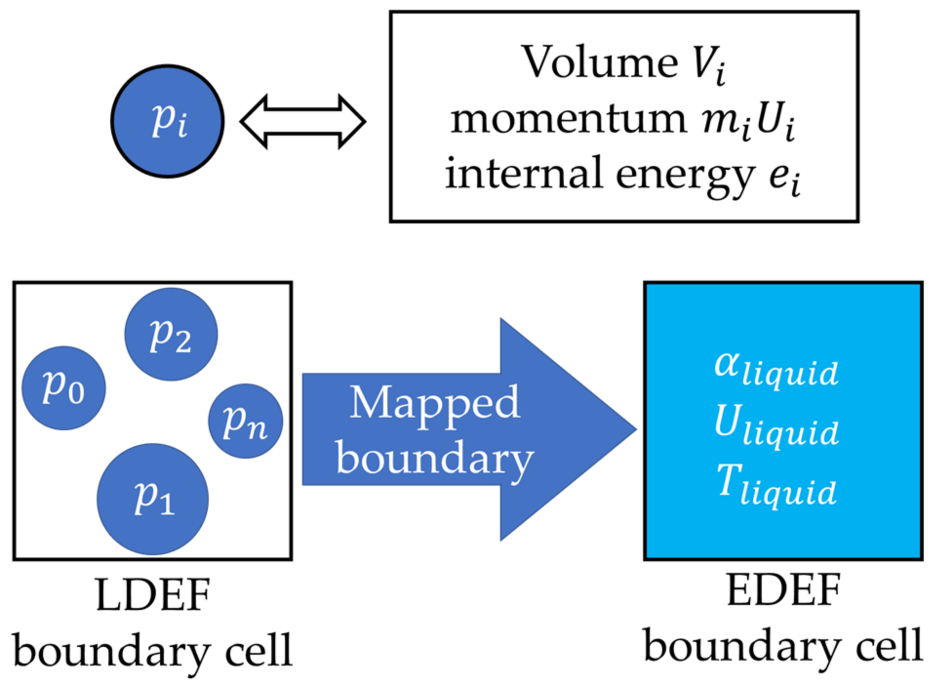
Creating a source file to map the data between the two regions using Equations (1)–(3).

Figure 5 summarizes the inner steps carried out at each time loop. At the beginning of the loop (blue blocks), the time steps for both regions are computed based on the maximum allowed CFL numbers $\left({\mathsf{\Delta }\mathrm{t} \mathsf{\Sigma }\mathrm{u}}_{{\mathrm{x}}_{\mathrm{i}}}/{\mathsf{\Delta }\mathrm{x}}_{\mathrm{i}}\right)$ set at the pre-processing phase.

Figure 5. Global steps carried out at each time loop.

Next, the algorithm sets the smaller time step for both regions. The LDEF step (red blocks) comprises solving Lagrangian and Eulerian equations.

The particle number is updated at each time step $n$, according to Equation (4). The update adds to the old particle number the newly injected particles and subtracts the particles absorbed by the EDEF region and particles which exit the computational domain:

$$P_n=P_{n-1}+P_{inj,n}-P_{abs,n}-P_{esc}$$

(4)

where $P$ refers to the particles’ numbers, the indexes $inj$, $abs$, and $esc$ refer to the injected, absorbed, and escaped particles, respectively.

The number of injected particles is computed following a pre-set flow rate and the particle diameter distribution. OpenFOAM provides several options for those two parameters. However, reference [7] validated the LDEF model for a constant flow-rate with a Rosin–Rammler distribution [16].

The conservation equations are solved using the PIMPLE algorithm of OpenFOAM [17]. Within one time-step, the algorithm searches for a steady-state solution with under-relaxation, then advances in time. The explicit parts of the equations are solved with three outer correction loops. After reaching a defined tolerance criterion of ${10}^{-6}$ within the steady-state calculation, the algorithm leaves the outer correction loop and advances in time.

The Lagrangian equations are analytically solved outside the pimple loop. Particles (or droplets) with identical properties, such as diameter and velocity, are associated in the same numerical parcels. Parcels are treated as point masses with no volume. Positions and velocities are updated at each time step, based on the momentum equation. Refinement is achieved by increasing the spray parcel rates. An increase in spray parcel rate diminishes the particle number represented by a single parcel, and augments the variety of particles. Further information about the Lagrangian equations can be found in [18]. The pimple loop encompasses the Eulerian equations for the LDEF region, the mapping equations, and the EDEF equations for both phases. Finally, the numerical schemes and algorithm controls presented in [7,8] are used.

4. Verifications and Calibration

The LDEF and EDEF equations have been validated in previous works ([7,8]). The verifications and calibration tests of the present article serve to:

i.

Verify the grid- and the parcel-rate-induced errors for the Lagrangian model. This verification serves to set an adequate mesh and parcel rate for the LDEF region and to generate reference data to assess momentum conservation for the multi-region approach.

ii.

Verify the STP predicted using the multi-region approach compared with the STP predicted using the Lagrangian approach. This test aims to verify the momentum transfer between the two regions.

iii.

Calibrate the permeability coefficient of the extended enthalpy–porosity technique according to the methodology suggested in [19].

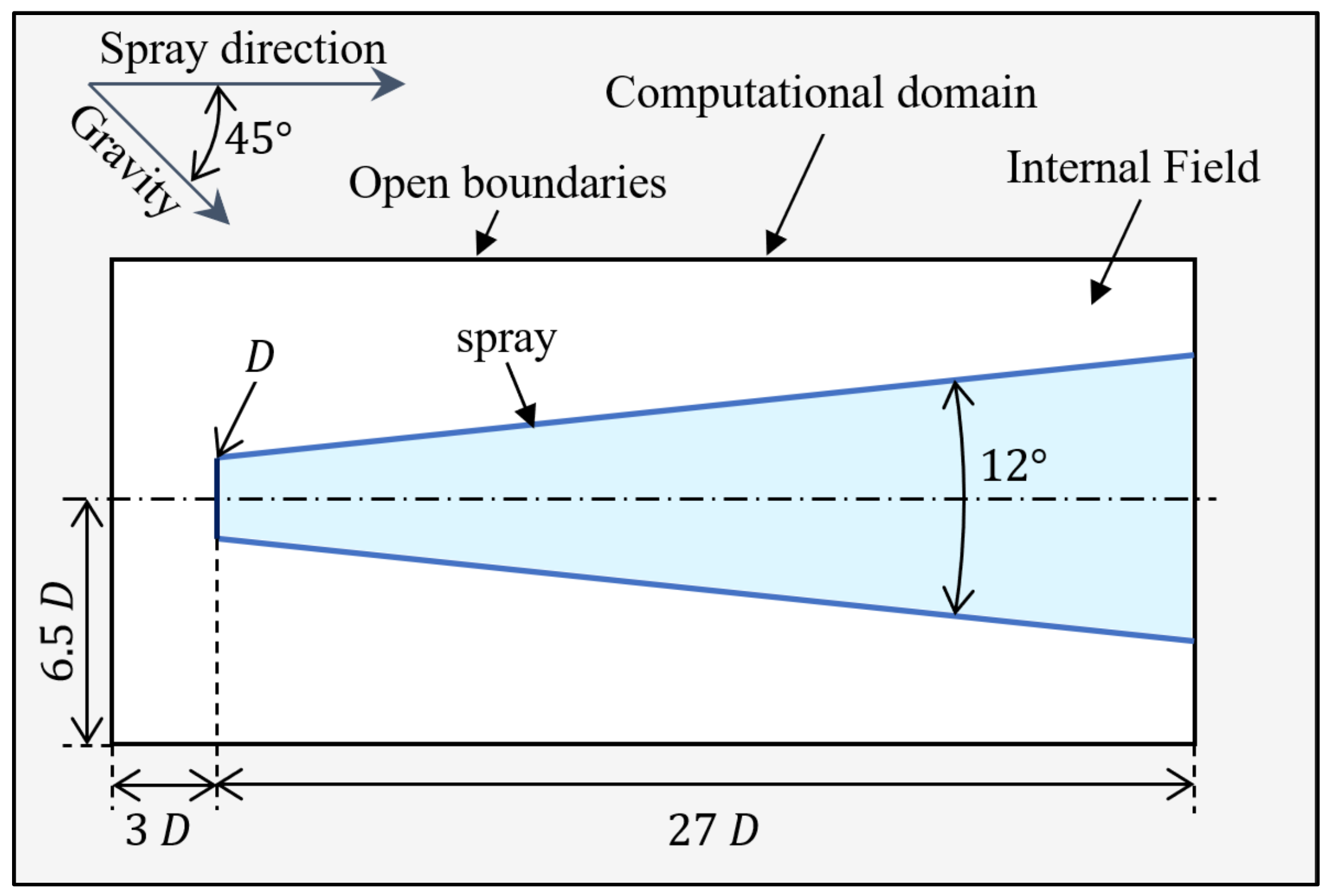
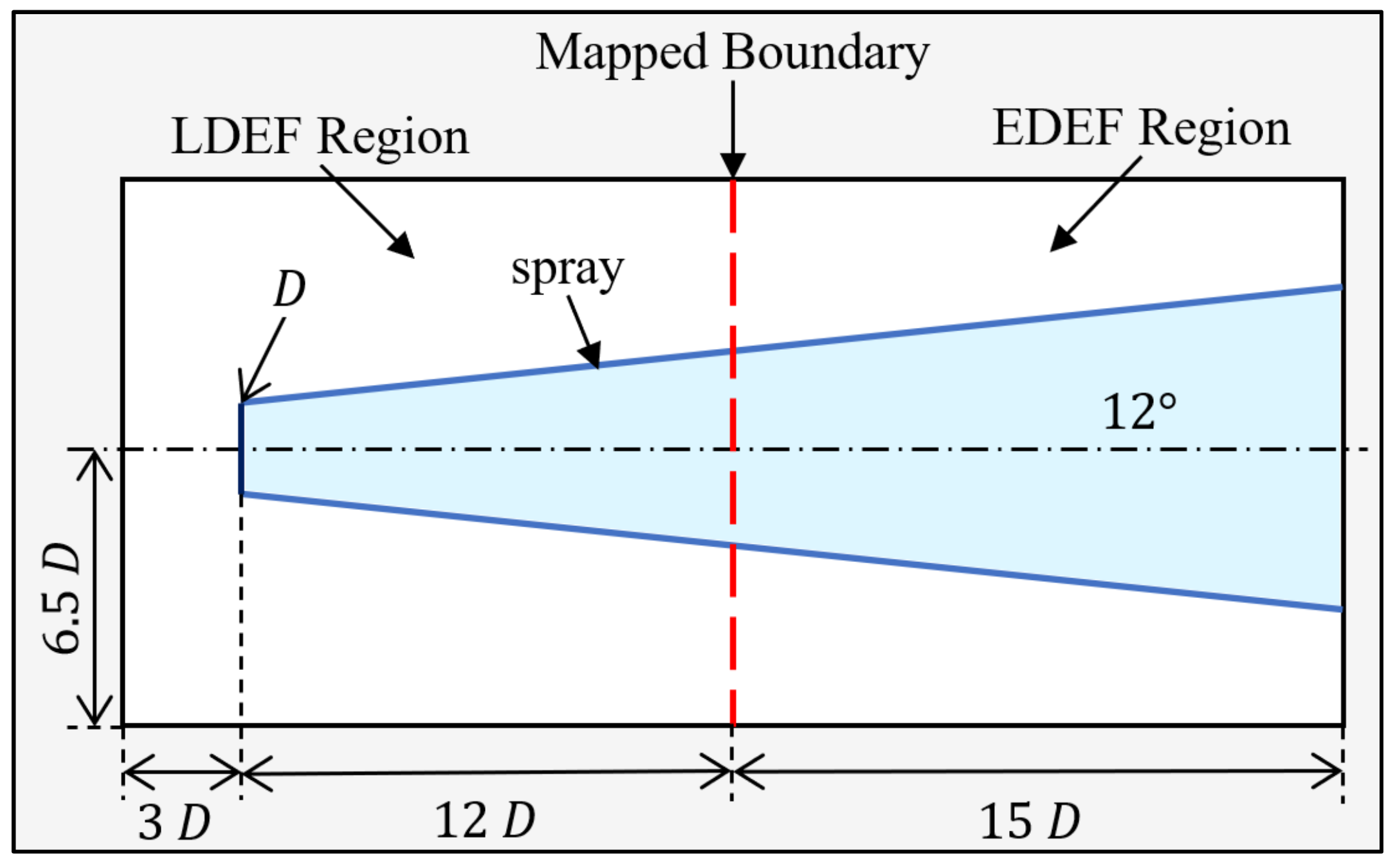
4.1. Spray Tip Penetration (STP) Test Case

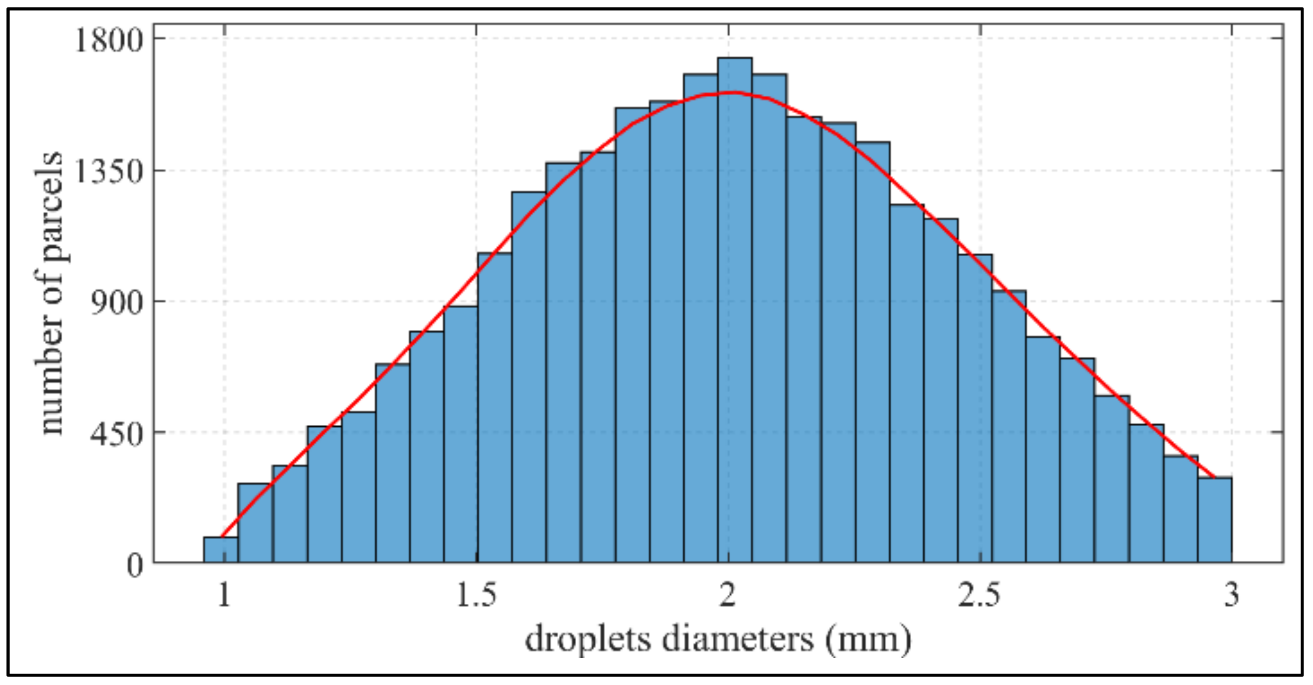
4.1.1. Injection Parameters

OpenFOAM’s Lagrangian framework injects particle spray without solving the flow inside the nozzle. The injected particle spray is characterized by a nozzle diameter, a flow rate, a particle size distribution, a spray pattern, a parcel rate, and an injection pressure. The inlet particle velocity is computed from the injection pressure and the ambient pressure.

Previous work [7] validated spray-tip penetration for a fuel spray against the experimental results of [20]. Unfortunately, ADF sprays have not been experimentally investigated in the literature. Therefore, the validation of the OpenFOAM’s Lagrangian framework in the context of ADF sprays is not yet possible. The main differences between the injection parameters for fuel and ADF sprays are summarized in Table 1.

Table 1. Differences between the injection parameters of fuel and ADF sprays.

Parameters	Fuel Sprays [20]	ADF Sprays
Injection pressure	120–200 bar	6 bar
Chamber pressure	1–12 bar	1 bar
Droplet mean diameter	15–25 μm	1–2 mm
Fluid viscosity	0.78 cSt	1 cSt
Fluid density	692 kg/m3	1113 kg/m3
Surface tension	0.0188 N/m	0.05 N/m

The principal difference comes from the higher injection pressure and the smaller droplets’ diameter in the case of fuel sprays. This leads to greater dispersion of the fuel injection spray.

The momentum conservation for the multi-region model was verified with realistic injection conditions. The SAE AS6285 [21] states that ADF injection pressure varies from one aircraft to another and from one aircraft part to another. However, the standardized international aircraft ground deicing program (SIAGDP) [22] suggests that equipment with $50–275 \mathrm{L}/\min$ flow rate at a pre-nozzle discharge pressure of $650 \mathrm{kPa}$ is suitable for any deicing task.

The nozzle BER-HT150 has a diameter of $38.1 \mathrm{mm}$ [23] and is approved by the SAE G-12 committee. The SAE G-12 committee serves as the focal point for all ground de-icing related activities within SAE. The nozzle’s manufacturer also specializes in designing firefighting nozzles; given the lack of experimental data for ADF spray, it is interesting to build an analogy between ADF sprays and firefighting sprays. Reference [24] validated a Lagrangian model for firefighting sprays. The spray parameters are similar to ADF spray parameters; an injection pressure of $600 \mathrm{kPa}$ with a nozzle diameter of $30 \mathrm{mm}$. However, the flow rate is higher ($1251 \mathrm{L}/\min$). Reference [24] used same size distribution (Rosin–Rammler) with three mean diameters, $0.5 \mathrm{mm}$, $1 \mathrm{mm}$, and $2 \mathrm{mm}$, and a 12-degree spray pattern. The SIAGDP [22] suggest using the largest droplet size to retain maximum heat in the ADF. Hence, the highest mean diameter presented in [24] was used. The computations were made using a Rosin–Rammler distribution of the droplet’s diameter between 1 mm and 3 mm, with a mean value of 2 mm, see Figure 6. Data were acquired by post-processing 29,502 parcels. The imposed probability distribution function (PDF) was scaled and is presented (by a red curve) on the same figure.

Figure 6. Histogram and scaled PDF of the Rosin–Rammler distribution.

Table 2 summarizes the injection parameters used in this test. In the following, the reference data were generated by grid and parcel-rate sensibility tests. Then, the precision of the multi-region approach was assessed through comparison with the reference data.

Table 2. Injection parameters.

Spray Parameters	Values
Nozzle diameter $\left(D\right)$	38.1 mm
Injection pressure	600 kPa
Flow rate	200 L/min
Mean droplet diameter	2.0 mm
Spray pattern	12°
Temperature	333.15 K

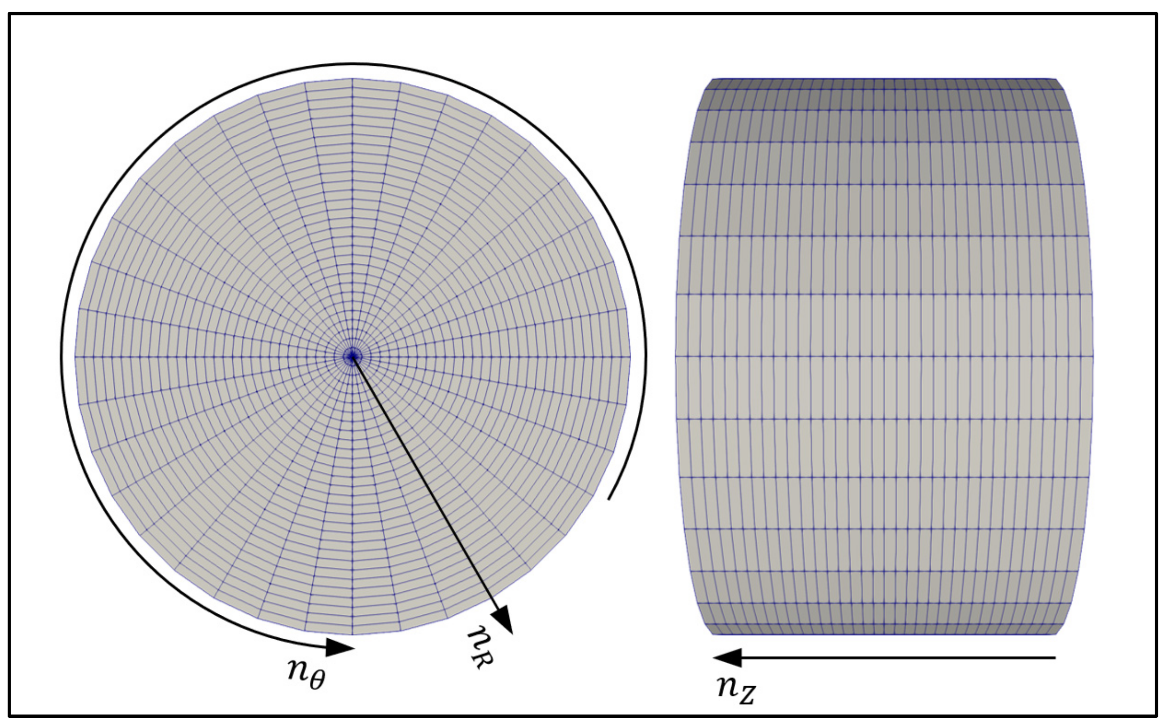
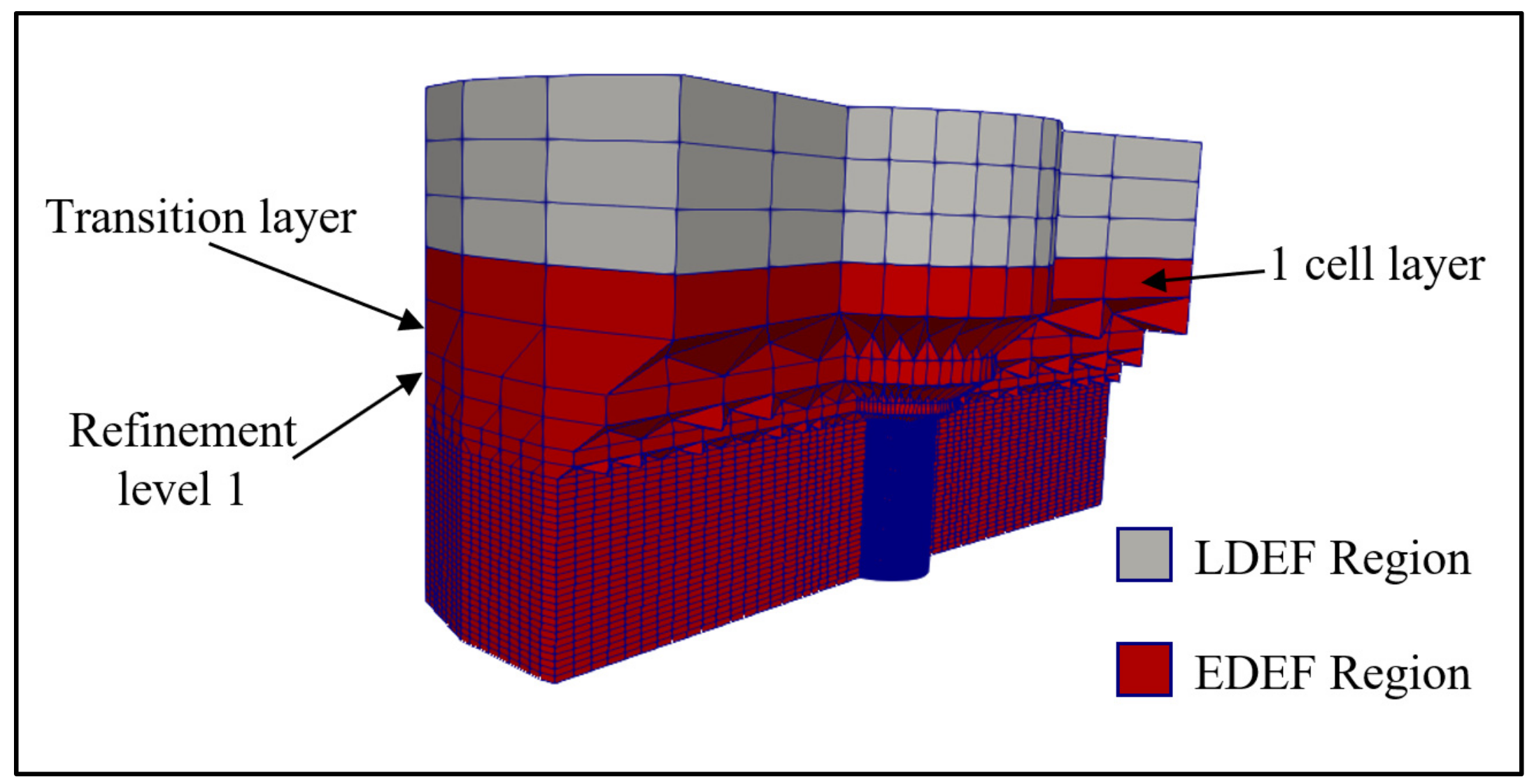
4.1.2. Computational Domain and Mesh

Figure 7 presents the computational domain for the STP test. The domain consisted of a cylinder with a length of $30 D$. The space between the nozzle tip and the boundaries was $3.0 D$ to avoid particle interactions with the boundary conditions at the injection. The spray-tip penetration was tracked along $27 D$, around $1.0 \mathrm{m}$. This spraying distance is typical of the AGD process [21].

Figure 7. Computational domain of the Lagrangian test case.

A domain diameter of 13 D ensured that spray droplets exited the cylindrical domain only through its base. The liquid spray evolved in the air (identified as “internal field” on the figure). The spray direction was at a $45°$ angle with gravity. To generate independent reference data from cell size and parcel size, twenty computations were performed using four meshes (presented in Table 3) and five parcel rates (${10}^3, {10}^4, {10}^5, {10}^6, {10}^7$).

Table 3. Reference Data Grids.

Meshes		${\mathit{n}}_{\mathit{R}}$	${\mathit{n}}_{\mathit{\theta }}$	${\mathit{n}}_{\mathit{Z}}$	Number of Cells
Mesh1	Coarse	13	16	60	12,480
Mesh2	Medium	20	24	90	43,200
Mesh3	Fine	30	36	135	145,800
Mesh4	Extra-Fine	45	60	200	540,000

Figure 8 presents a 25% grid section (axis length of $7.0 D$). The grid was parametrized through three variables: the number of cells in the radius direction $\left(n_R\right)$, the number of cells in the angular direction $\left(n_{\theta }\right)$, and the number of cells in the axis direction $\left(n_Z\right)$.

Figure 8. Typical mesh section.

4.1.3. Thermophysical Model

ADFs are composed mainly of ethylene glycol. They also contain corrosion inhibitors and other fluids to reduce their surface tension and increase their viscosity. Their composition can vary depending on the manufacturer. For simplicity, ADFs in this paper are pure ethylene glycol. The internal field is composed of three species: dioxygen $O_2$, dinitrogen $N_2$, and ethylene glycol vapor $C_2{H}_6{O}_2$. These species are weighted by $Y_{specie}$ and are a function of the temperature. The density is computed using the perfect gas law presented in Equation (5):

$$\rho ={\displaystyle \sum }_{species}{Y}_{specie}\times \frac{M_{species}}{RT}p$$

(5)

where $M_{species}$, $R$, and $p$ refer, respectively, to the species’ molar weight, the fluid constant, and the pressure field.

The specific heat capacity of each species is computed in Equation (6) as a function of the temperature following the NIST-JANAF thermochemical tables [25]:

$$C_p=\sum \left(Y_{specie}\left(a_4{T}^4+a_3{T}^3+a_2{T}^2+a_{1}T+a_0\right)\right)$$

(6)

Finally, the dynamic viscosity follows the Sutherland law presented in Equation (7):

$$\mu =\frac{A_s\sqrt{T}}{1+T_s/T}$$

(7)

The parameter values used in Equations (5)–(7) are presented in Table 4.

Table 4. Internal Field Thermophysical Parameters.

	${\mathit{N}}_2$	${\mathit{O}}_2$	${\mathit{C}}_2{\mathit{H}}_6{\mathit{O}}_2$
$M\left({\mathrm{kg} \mathrm{m}}^{-3} \right)$	$28.01$	$32.00$	$62.07$
$A_s\left({\mathrm{kg} \mathrm{m}}^{-1}{ \mathrm{s}}^{-1}{ \mathrm{K}}^{-1} \right)$	$1.67 \times {10}^{-6}$	$1.67 \times {10}^{-6}$	$1.67 \times {10}^{-6}$
$T_s \left(\mathrm{K}\right)$	$171$	$171$	$171$
$a_0 \left({10}^0\right)$	$3.30$	$3.21$	$1.97$
$a_1 \left({10}^{-3}\right)$	$1.41$	$1.13$	$2.02$
$a_2 \left({10}^{-6}\right)$	$-3.96$	$-5.76$	$-3.70$
$a_3 \left({10}^{-9}\right)$	$5.64$	$1.31$	$4.05$
$a_4 \left({10}^{-12}\right)$	$-2.44$	$-0.88$	$-1.46$

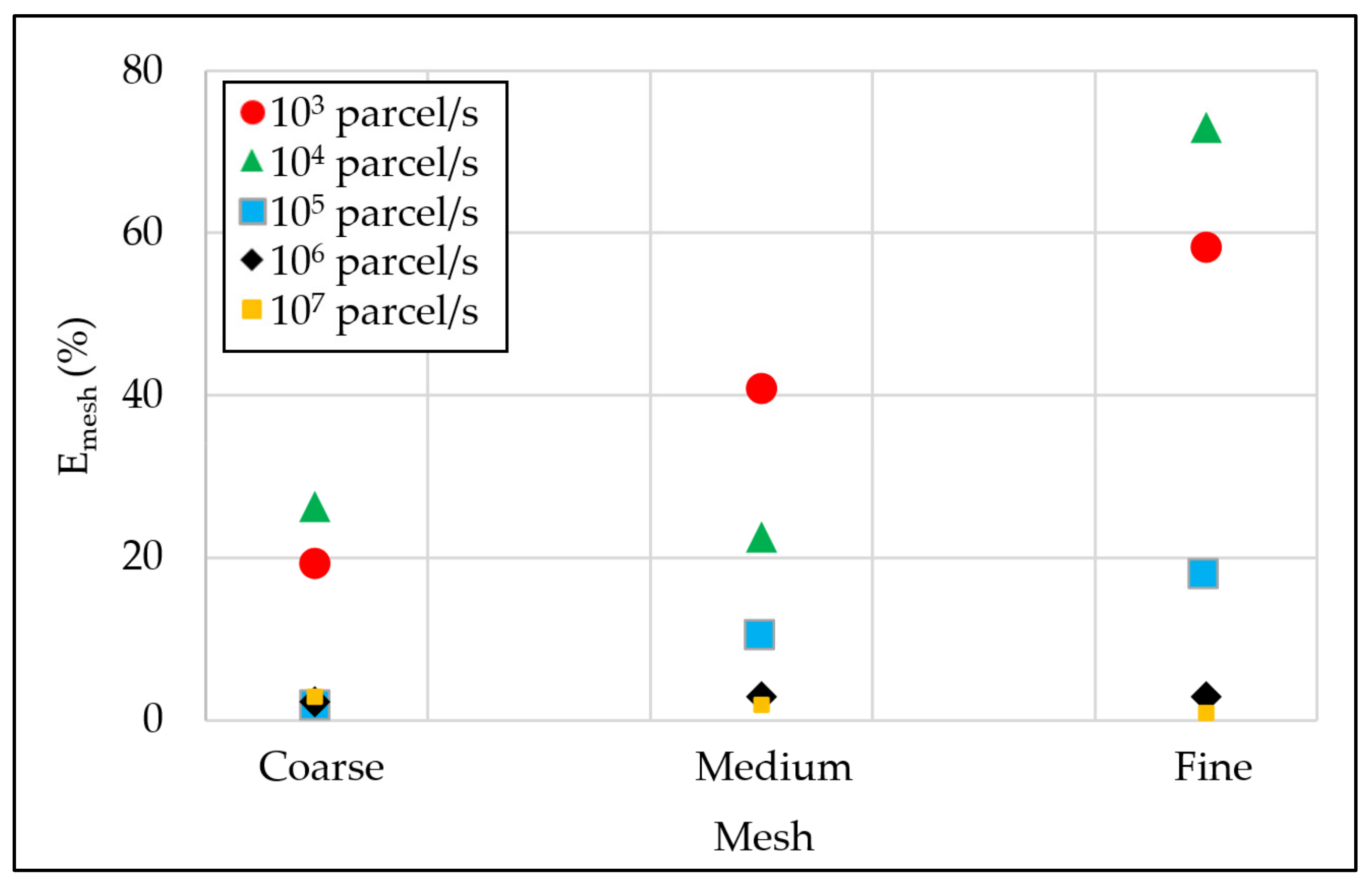
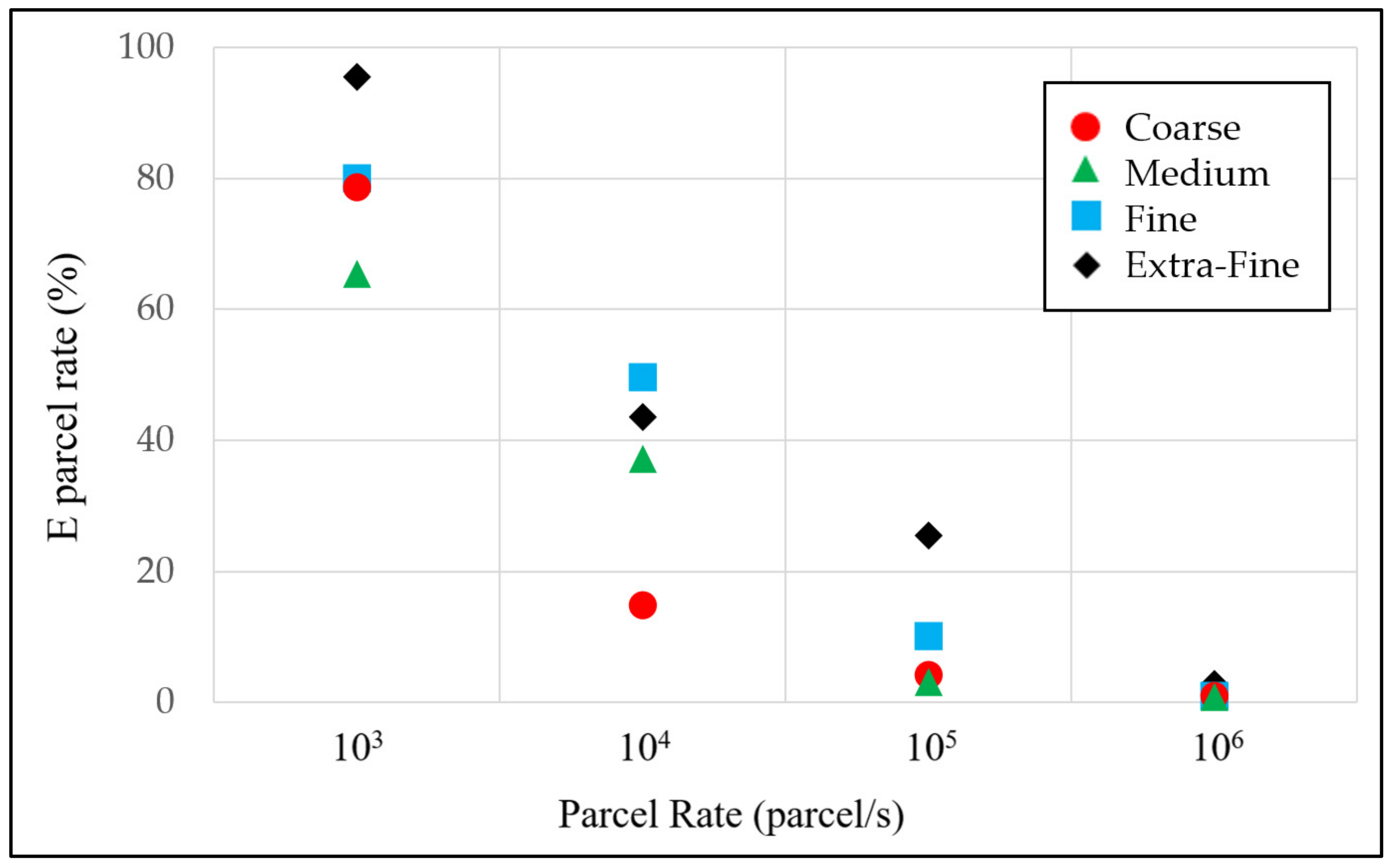
4.1.4. Parcel Rate Sensitivity

The STP is defined as the height of a cylinder coaxial with the spray axis. The cylinder encompassed 95% of the spray’s total mass. To assess STP sensitivity to the spray parcel rate (PR), a parcel-rate-induced error $\left(E_{PR}\right)$ is defined. Equation (8) expresses the PR-induced error for a mesh $“m_i”$and a PR $“P{R}_j”$:

$$E_{PR}\left(m_i, P{R}_j\right)=\frac{1}{M_{ij}}\underset{t_0}{\overset{t_f}{{\displaystyle \int }}}\left|STP\left(m_i, P{R}_{j+1}\right)-STP\left(m_i, P{R}_j\right)\right|$$

(8)

where $M_{ij}=\left(t_f-t_0\right)· \underset{\mathrm{time}}{\max }\left(STP\left(m_i, P{R}_j\right)\right)$ with $t_0$ and $t_f$ respectively the initial and final time of the simulation.

Figure 9 presents the PR-induced error for the four meshes. Increasing the PR decreased the error for the four meshes. The STP sensitivity to the PR increased when the mesh was refined. The coarse mesh presented a sensitivity under 20% for a PR of ${10}^4 \mathrm{parcel}/\mathrm{s}$, whereas the extra-fine mesh continued to present a sensitivity above 20% for a PR 10 times greater. For a PR of ${10}^6 \mathrm{parcel}/\mathrm{s}$, all the four meshes presented almost the same PR-induced errors of $1\%$, except the extra-fine mesh which presented an error of 3%. Therefore, the PR of ${10}^6 \mathrm{parcel}/\mathrm{s}$ was retained for the spray configuration. The next paragraph analyzes the grid induced error for selection of the appropriate mesh.

Figure 9. STP sensitivity to the parcel rate for the four meshes.

4.1.5. Grid Sensitivity

To assess the spray tip penetration (STP) sensitivity to the mesh, a grid-induced error $\left(E_m\right)$ was defined. Equation (9) expresses the grid-induced error for a $\mathrm{PR}$ $“P{R}_i”$, and a mesh $“m_j”$:

$$E_m\left(P{R}_i, m_j\right)=\frac{1}{M_{ij}}\underset{time}{\overset{}{{\displaystyle \int }}}\left|STP\left(P{R}_i, m_{j+1}\right)-STP\left(P{R}_i, m_j\right)\right|$$

(9)

Figure 10 presents the grid-induced error for the five tested PRs. For the “low” PRs of ${10}^3$ and ${10}^4$, the grid-induced errors were higher than for other PRs. The mesh refinement also increased the grid-induced error. The “high” PRs of the ${10}^6$ and ${10}^7$ STP predictions were almost independent of the mesh quality, both presenting a grid-induced error around $2\%$. Using a PR of ${10}^6 \mathrm{parcel}/\mathrm{s}$ allowed use of any of the studied meshes. The medium mesh was retained for the subsequent tests.

Figure 10. STP sensitivity to mesh quality rate for the five spray rates.

In the next paragraph, the multi-region approach is verified against the retained configuration of the Lagrangian approach i.e., a medium mesh with a parcel rate of ${10}^6 \mathrm{parcel}/\mathrm{s}$.

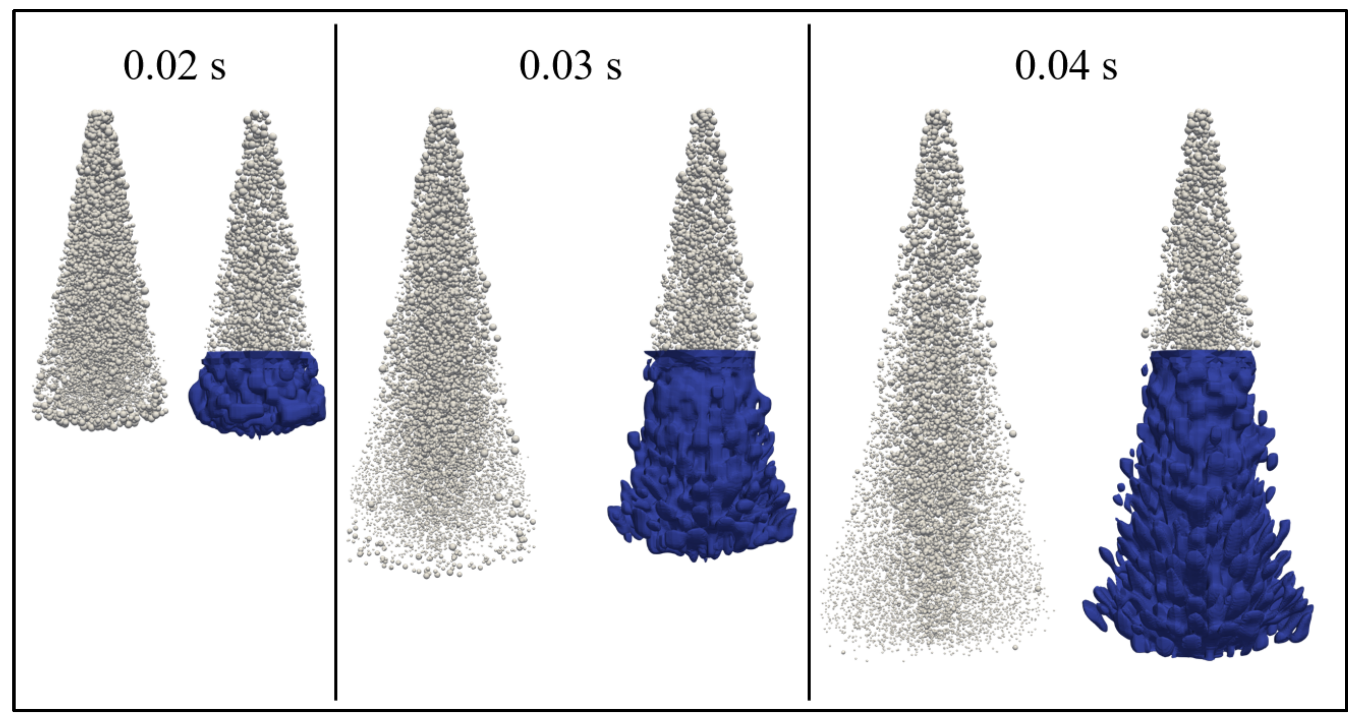
4.1.6. Multi-Region Validation

This paragraph compares the STP predicted using the multi-region approach to the STP predicted using the Lagrangian approach. Figure 11 presents the computational domain for the multi-region test case. The computational domain in Figure 7 is divided into two regions. The mapped boundary is located at the middle of the domain axis. The computation used the same boundary conditions, initial conditions, and injection parameters.

Figure 11. Computational domain of the multi-region test case.

The medium mesh was used first. Then, the EDEF region’s mesh was refined until reaching STP grid insensitivity. Figure 12 presents a crinkle clip of the mesh refinement architecture at three levels of refinement. The LDEF region’s mesh and the first cell layer after the mapped boundary are unedited. The second cell layer of the EDEF region is a transition layer where each cell was divided into four according to the radial and angular directions. In the third layer, each cell was divided into two according to the axis direction. The mesh in this layer kept the topology of the original mesh with eight times more cells. The same refinement strategy was repeated for the second and third meshes. The three meshes presented in Table 5 were used to study STP sensitivity to the meshes in this multi-region approach.

Figure 12. Mesh refinement architecture.

Table 5. Multi-Region Grids.

Mesh Id.	Number of Refinements	Number of Cells
Mesh 1	0 (medium mesh)	43,200
Mesh 2	1	184,320
Mesh 3	2	1,316,640

Equation (10) defines an error function, based on the STP reference values for the pure Lagrangian case $\left(ST{P}_{ref}\right)$:

$$error\left(m_i,t\right)=\frac{1}{\underset{\mathrm{time}}{\max }\left(ST{P}_{ref}\left(t\right)\right)}\left|STP\left(m_i,t\right)-ST{P}_{ref}\left(t\right)\right|$$

(10)

Figure 13 presents the computed error for the three meshes. The error was null until 0.016 s because the spray was evolving only in the LDEF region.

Figure 13. Muti-region model STP prediction error for the three meshes.

After the spray reached the mapped boundary, the error function increased. For the mesh without refinement (Mesh 1), the error was remarkably higher than that for the other meshes. The maximal errors for the three meshes were 10.4%, 1.50%, and 1.10%. The EDEF approach was more sensitive to the mesh than the LDEF approach.

Figure 14 presents three snapshots of the computed spray at three different times: 0.02 s, 0.03 s, and 0.04 s. The multi-region-computed spray (with two levels of refinement) is presented versus the Lagrangian spray (with a medium mesh and ${10}^6 \mathrm{parcel}/\mathrm{s}$). The blue cells are in the EDEF region; the grey spheres are parcels in the LDEF region. The figure illustrates the agreement between the two computations for both the STP and the spreading angle.

Figure 14. Spray evolution (Lagrangian versus multi-region).

4.2. Permeability Coefficient Calibration

The extended enthalpy–porosity technique was used to model the ice melting [8]. The Darcy law defines a permeability coefficient to approximate the velocity damping in the mushy region. The predicted thermal field depends on the permeability coefficient values [26].

The permeability coefficient $\left(Cu\right)$ appears in the momentum equation as a source term $\left(\mathit{S}=-Cu·\frac{{\delta }^2}{{\left(1-\delta \right)}^3+q} \mathit{u}\right)$, where $\delta$ is the solid fraction. If $\delta =0$, the source term vanishes. If $\delta =1$, the source term is equal to $\left(\frac{-Cu}{q}u\right)$, where $q={10}^{-3}$ is a model coefficient to avoid division by 0, but small enough for the source term to dominate other terms in the momentum equation, giving ($\mathit{u}=\mathbf{0})$. In the mushy region ($0<\delta <1$), the permeability coefficient directly affects the velocity’s predicted value.

The methodology suggested in [19] for the original enthalpy–porosity technique was used to calibrate the permeability coefficient, requiring adjustment of the permeability coefficient for every set of boundary conditions. This methodology had been used to calibrate the permeability coefficient of the extended enthalpy–porosity technique in 2D [8]. Because the present paper deals with 3D computations and a new set of boundary conditions, a recalibration was needed.

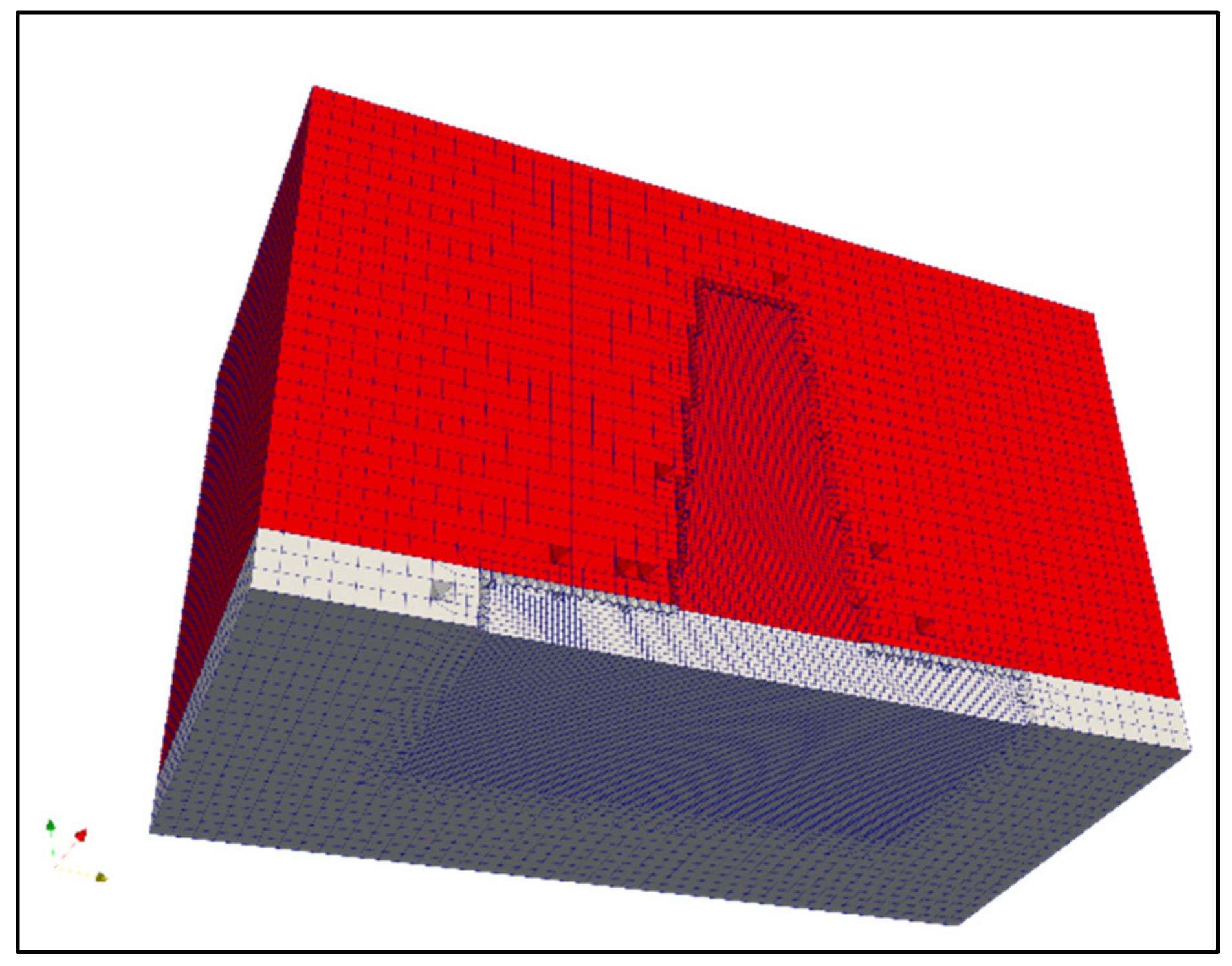
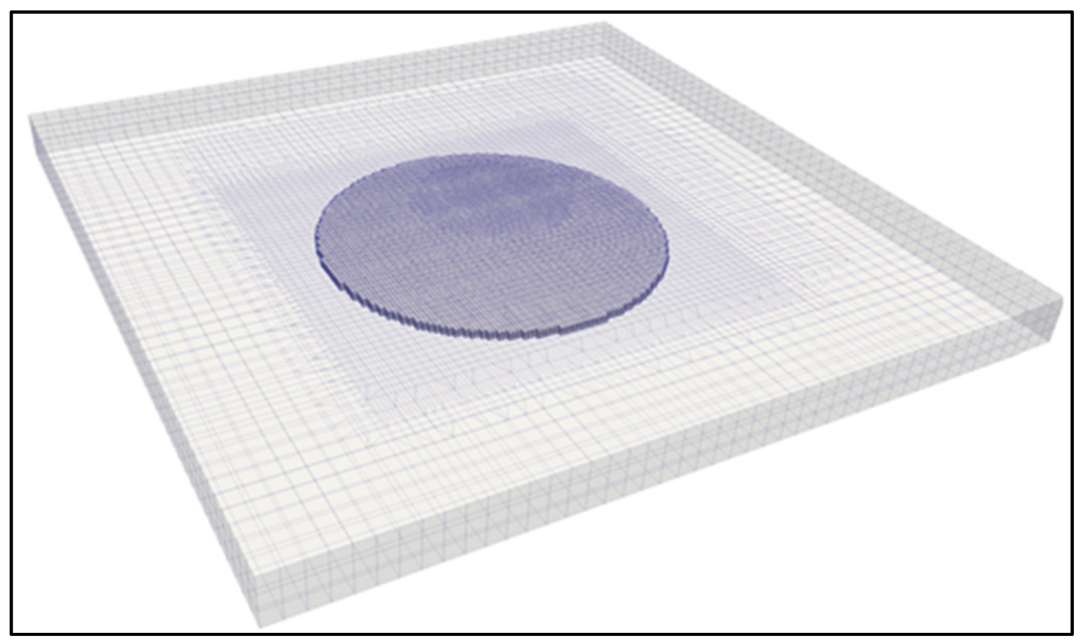
4.2.1. Test Case Setup and Meshes

The test case was a flat plate decontamination based on the spray parameters presented in Section 4.1.1. The computational domain consisted of a square cuboid ($45\mathrm{D}\times 45\mathrm{D}\times 38\mathrm{D}$). The upper and lateral patches were set to be atmospheric outlets, and the lower patch was a wall. The nozzle outlet was placed at $27\mathrm{D}$ (approximately 1 m) from the wall. Figure 15 presents a crinkle clip of the coarse mesh. The domain was meshed using cubic cells of $4/3\mathrm{D}$ edges. The mesh was then refined twice to obtain a cell size of $\mathrm{D}/3$ surrounding the liquid flow. The lateral boundaries were located at 8.5D, far enough from the contaminated area to avoid the reflective effects of boundary conditions. The mapped boundary was set at 4D from the wall. The LDEF cells are shown in red and the EDEF cells in grey. An ice cylinder, with a diameter of $28\mathrm{D}$ and a height (thickness) of $2/3\mathrm{D}$ (Figure 16), was located at the wall center at the start of the calculations.

Figure 15. Coarse mesh clip for the flat plate decontamination test case.

Figure 16. Ice zone in the EDEF region.

From the calibration, the result of interest is the ice volume’s change over time. Four meshes and four permeability coefficient values were tested for the calibration. The different meshes were obtained by refinement around the icy zone cells. The cell edges were divided by two, such that the cell edges were D/3, D/6, D/12, and D/24 for the coarse, medium, fine, and extra-fine meshes, respectively.

For the permeability coefficient, values in the literature range between ${10}^3$ and ${10}^{15}{ \mathrm{kg} \mathrm{s}}^{-1}{ \mathrm{m}}^{-3}$. However, values between ${10}^4$ and ${10}^8$ are often applied [19]. In this study, four values (${10}^4, {10}^5, {10}^6, \mathrm{and} {10}^7$) were tested.

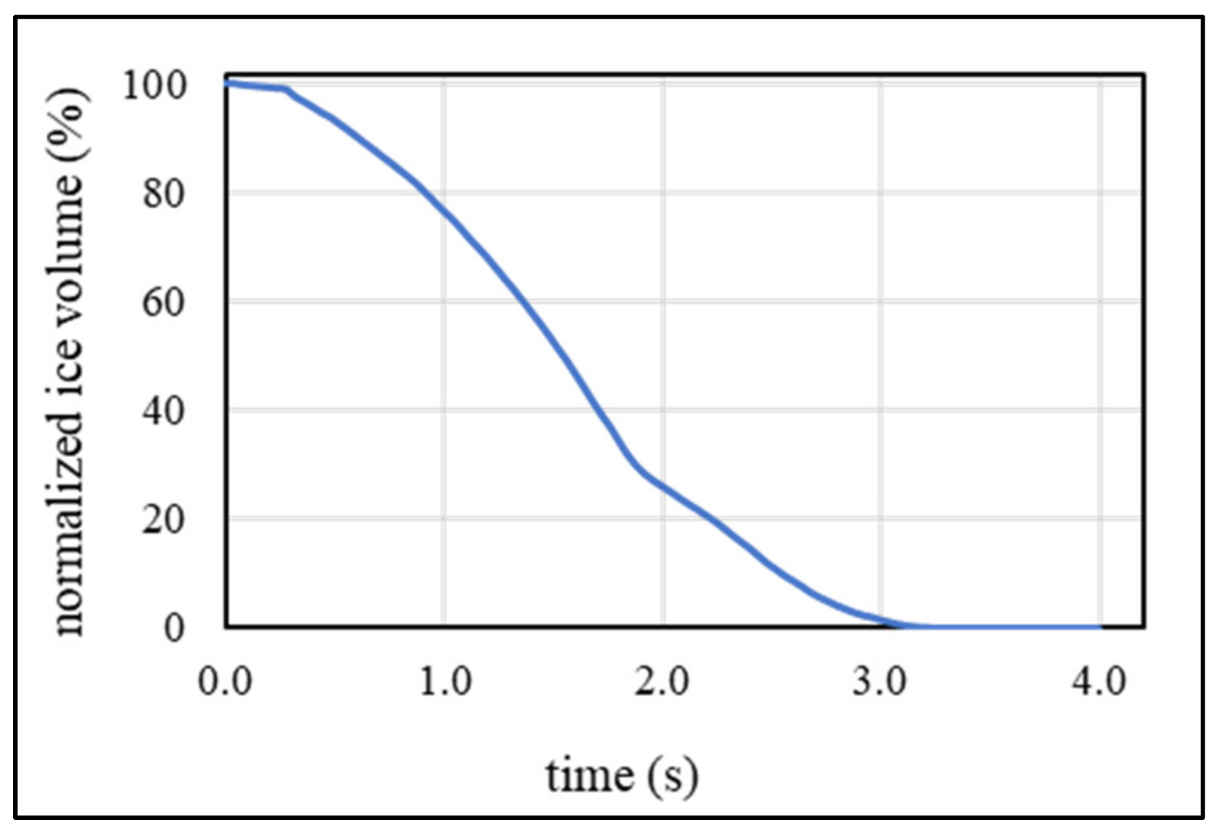
4.2.2. Results and Analysis

The effects of the mesh and the permeability coefficient on the ice volume evolution are presented. The ice volume $V_{ice}\left(t\right)$ is defined in Equation (11) as the summation of the ice volume over the computational domain:

$$V_{ice}\left(t\right)={\displaystyle \sum }_{cells}{V}_{cell}·{\delta }_{cell}\left(t\right)$$

(11)

where $V_{cell}$ is the cell volume and ${\delta }_{cell}\left(t\right)$ is the ice volume fraction in a cell at time $t$.

The normalized ice volume is computed with Equation (12):

$${\overline{V}}_{ice}\left(t\right)=100·\frac{V_{ice}\left(t\right)}{V_{ice}\left(0\right)}$$

(12)

All the computations were performed for 4 s (physical time). This duration is fixed based on the computations on the coarse mesh and a permeability coefficient of ${10}^6{ \mathrm{kg} \mathrm{s}}^{-1}{ \mathrm{m}}^{-3}$, which is the calibrated value for the 2D computations [8]. Figure 17 presents the ice volume evolution for the reference case. The flat plate was fully decontaminated after $3.32 \mathrm{s}$ of injection time.

Figure 17. Ice volume evolution (reference case).

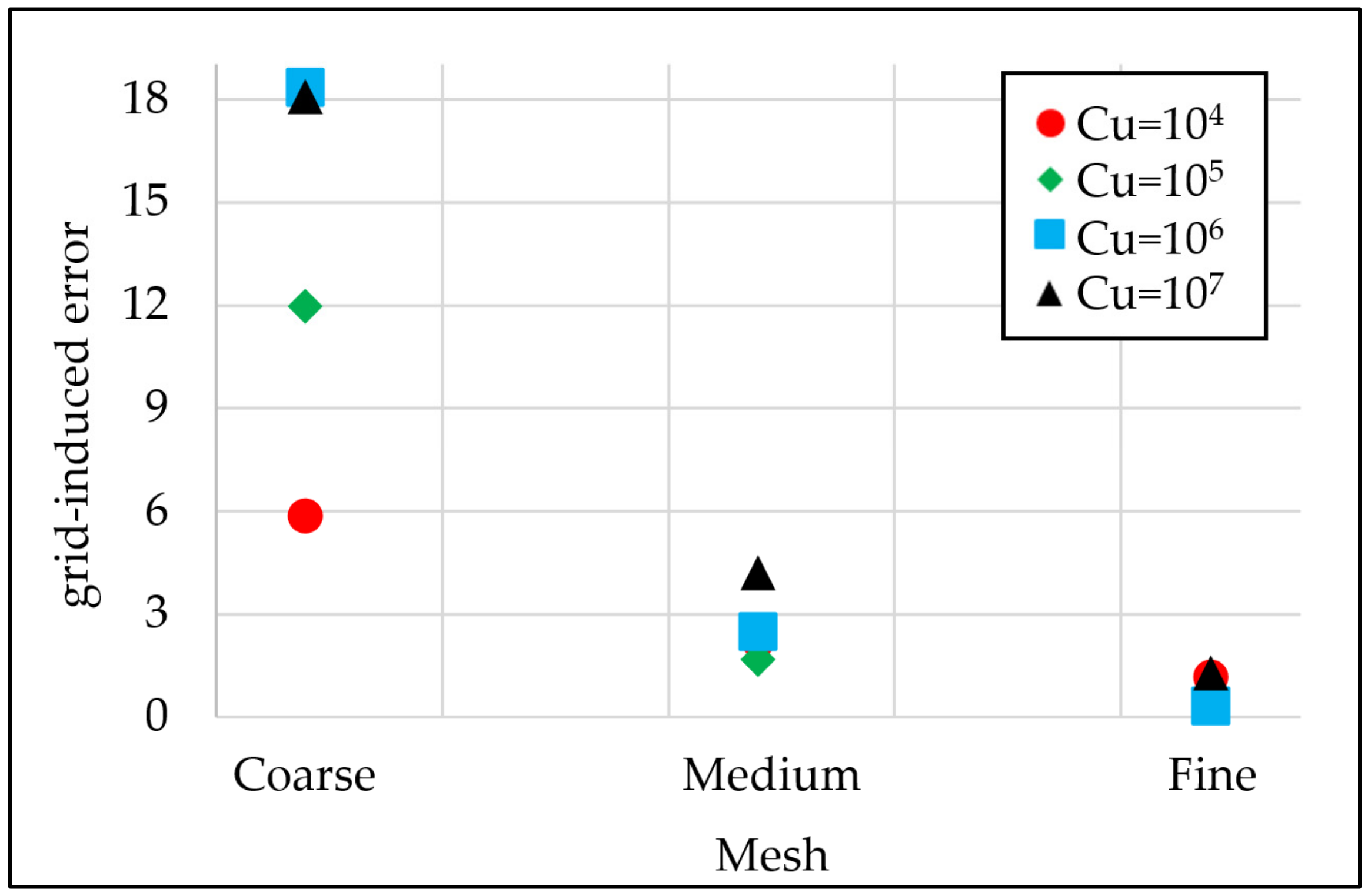
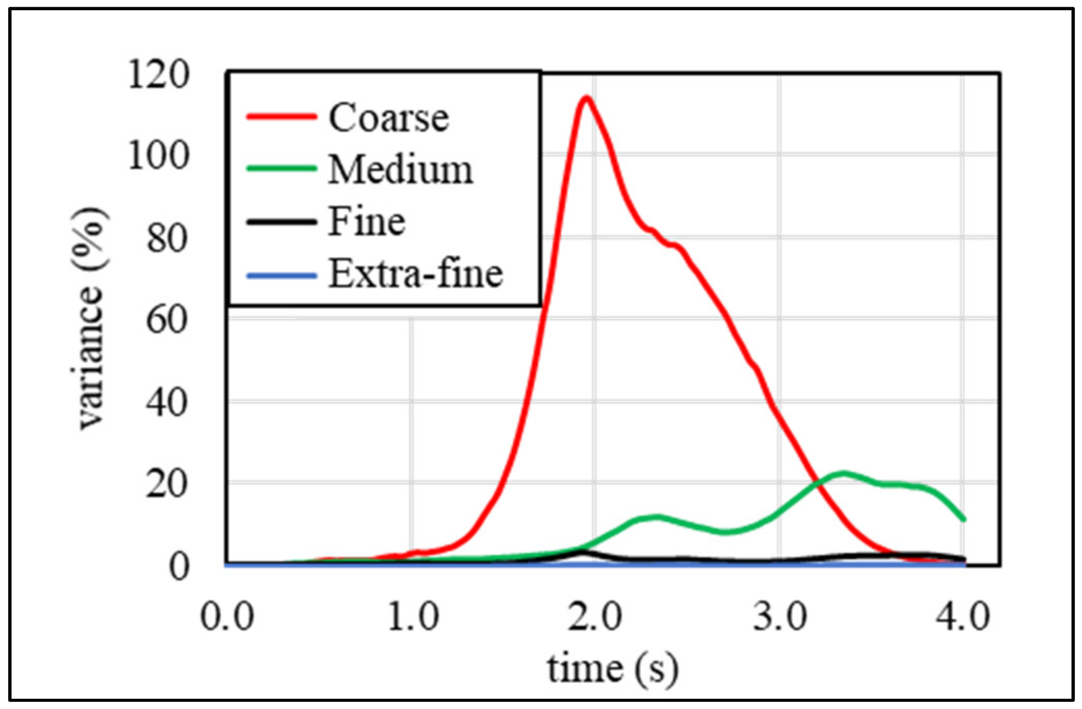
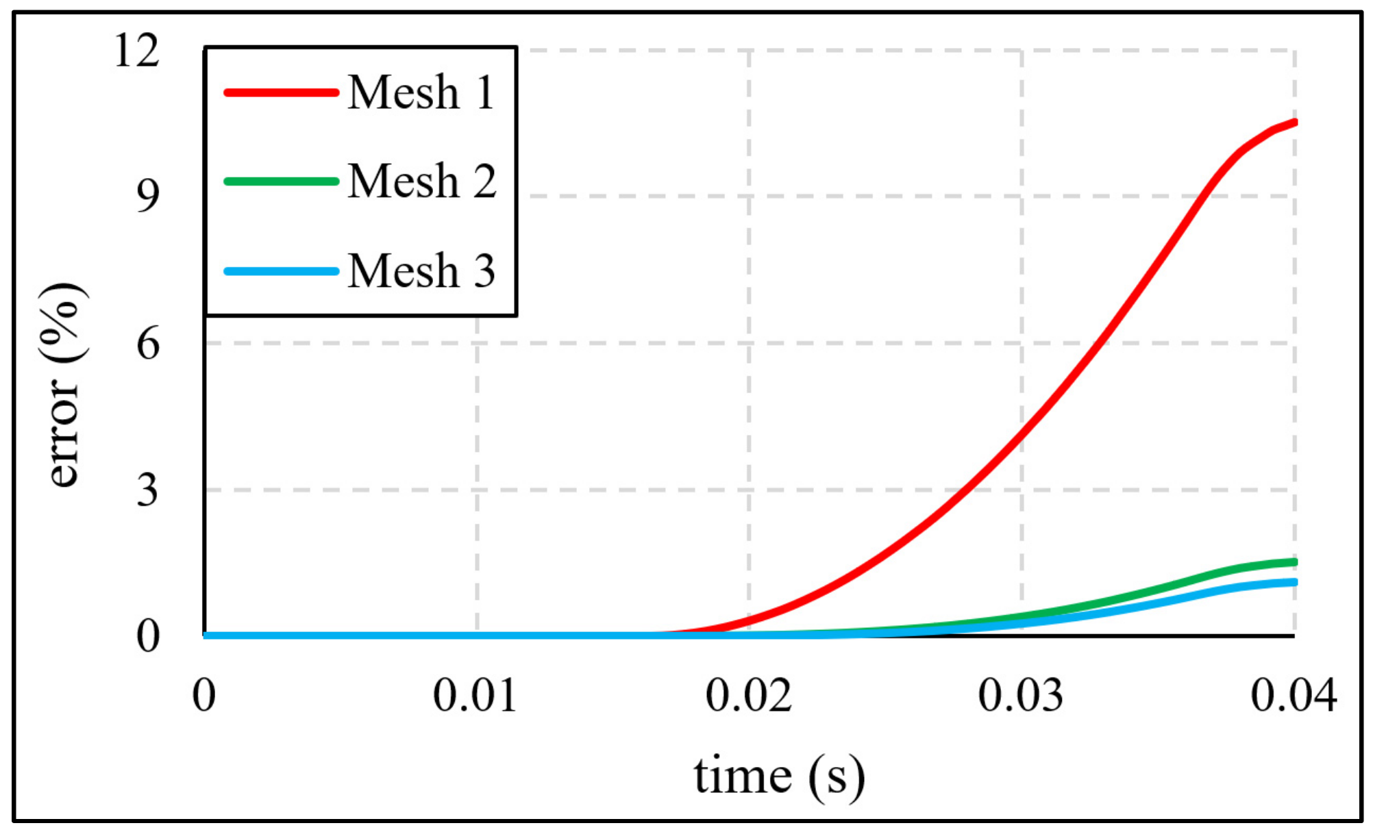
4.2.3. Grid Sensitivity

For the grid sensitivity study, a grid-induced error $\left(E_m\right)$ is defined as a function of the permeability coefficient $\left(C{u}_i\right)$ and the mesh $(m_j)$ in Equation (13):

$$E_m\left(C{u}_i, m_j\right)=\frac{1}{\mathrm{total} \mathrm{time}}\underset{time}{\overset{}{{\displaystyle \int }}}\left|{\overline{V}}_{ice}\left(C{u}_i, m_{j+1}\right)-{\overline{V}}_{ice}\left(C{u}_i, m_j\right)\right|$$

(13)

Figure 18 presents the grid-induced error for the four tested permeability coefficients. The computation results were more sensitive to the mesh for the higher permeability coefficients. Except for the permeability coefficient of ${10}^7$, the grid-induced error was lower than 3% for the medium mesh. For the fine mesh, the permeability coefficients of ${10}^5$ and ${10}^6$ gave errors of 0.26% and 0.34%, respectively. The permeability coefficients of ${10}^4$ and ${10}^7$ generated errors of 1.23% and 1.29%, respectively.

Figure 18. Ice volume evolution sensitivity to mesh quality for the four tested permeability coefficients.

In the engineering context, a grid-induced error of 3% is acceptable. For the fine mesh, the grid induced error for the four tested permeability coefficients was acceptable. The fine mesh is mandatory to ensure a grid-induced error below 3% for a permeability coefficient of ${10}^7$. The best compromise between accuracy and computation cost could be found in the medium mesh and a permeability coefficient of ${10}^5$. This setup had a grid-induced error of only 1.66%. Furthermore, for faster computations and model simplicity, the evaporation in the LDEF region could be neglected since only 0.27% of the injected mass evaporated.

4.2.4. Permeability Coefficient Sensitivity

The instantaneous variance of the normalized ice volume, computed with Equation (14), assesses the permeability coefficient sensitivity. The distance to the mean value, $d\left(C{u}_i,m_j,t\right),$is computed with Equation (15):

$${\sigma }^2\left(m_j,t\right)=\frac{{{\displaystyle \sum }}_{i=1}^4{d}^2\left(C{u}_i,m_j,t\right)}{3}$$

(14)

$$d\left(C{u}_i,m_j,t\right)={\overline{V}}_{ice}\left(C{u}_i,m_j,t\right)-{\displaystyle \sum }_{k=1}^4\left(\frac{{\overline{V}}_{ice}\left(C{u}_k,m_j,t\right)}{4}\right)$$

(15)

Figure 19 presents the normalized ice volume variance for the four meshes. The overall variance $\left({{\displaystyle \int }}_t^{}{\sigma }^2\left(m_j,t\right)dt\right)$decreased with mesh refinement. The ice volume was less sensitive to the permeability coefficient for the finer meshes, as presented in [19]. The maximum variances for the fine and extra-fine meshes were 3.32% and 0.02%, respectively. Results for the extra-fine mesh were almost insensitive to the permeability coefficient.

Figure 19. Normalized ice volume variance for different meshes.

Table 6 indicates the average distance to the mean value and the results helped to select a case setup. This average distance is the temporal average of the distance defined by Equation (15).

Table 6. Average distance to the mean values for different meshes.

	$\mathit{C}\mathit{u}={10}^4$	$\mathit{C}\mathit{u}={10}^5$	$\mathit{C}\mathit{u}={10}^6$	$\mathit{C}\mathit{u}={10}^7$
Coarse	12.68	3.23	5.73	29.69
Medium	5.27	0.10	1.52	7.60
Fine	0.40	0.14	0.41	1.13
Extra-fine	0.08	0.11	0.40	0.76

For all meshes, a permeability coefficient of ${10}^5$ represented the smallest distance. For a medium mesh with a permeability coefficient of ${10}^5$, the grid-induced error was 1.66%. A suitable compromise between computer time and accuracy was reached with a permeability coefficient of ${10}^5$ using a medium mesh.

5. Conclusions

A new OpenFOAM-V6 based solver $\left(AGDFoam\right)$ has been developed and verified to simulate the AGD process. The new solver is a combination of the native solver $\left(sprayFoam\right)$ and the $\left(AGDEulerFoam\right)$ solver developed in [8]. The new solver has been designed for simulating the AGD process in 3D. In this paper, a set of injection parameters is proposed on the basis of a technical review. A computational domain divided into two regions enabled the simulations. The first region was designed for the spray evolution far from the wall, and the spray evolution was solved using a Lagrangian approach. The flow in the second region was modelled with the Eulerian approach. The second region was designed to model the ice decontamination. For the multi-region approach, the momentum conservation was verified through a spray-tip penetration (STP) test case. The STP sensitivity to the PR and the mesh was studied. The permeability coefficient of the extended enthalpy–porosity technique was then calibrated. For the proposed injection parameters, it was concluded that:

• Using a PR superior to ${10}^6 \mathrm{parcel}/\mathrm{s}$ brings the computations to independency from the mesh density in the Lagrangian region.
• Computations in the Eulerian region are more sensitive to the mesh density. The grid is acceptable for a mesh eight times finer than the medium mesh.
• A permeability coefficient of ${10}^5$ ${\mathrm{kg} \mathrm{s}}^{-1} {\mathrm{m}}^{-3}$ gives a good prediction (2%) using a medium mesh. For enhanced accuracy, it is advised to multiply the number of mesh elements by eight to reach results that are almost insensitive to the permeability coefficient.

This paper is part of a research effort to design a CFD test bench for the AGD process. For the first time, this study used realistic injection parameters for the AGD spray. The multi-region approach conserved the STP evolution profile predicted using the Lagrangian solver, which verified the momentum transfer methodology applied between the two regions. Future works will focus on studying the influence of the spray parameters on the ice decontamination rate.

Appendix A.1. LDEF Region Governing Equations

The mass conservation equation of the LDEF region is given by the following equation:

$$\frac{\partial \rho }{\partial t}+\nabla .\left(\rho \mathit{u}\right)=\frac{{\dot{m}}_{p,evap}}{V_{Cell}}$$

(A1)

where ${\dot{m}}_{p,evap}$ is a mass source term generated by the evaporation of spray particles.

The momentum conservation in the LDEF region is given by the following equation:

$$\frac{\partial \rho \mathit{u}}{\partial t}+\mathbf{\nabla }.\left(\rho \mathit{u}\mathit{u}\right)=-\mathbf{\nabla }p+\rho \mathit{g}+\mathbf{\nabla }.\left(2{\mu }_{eff}D\left(\mathit{u}\right)\right)-\mathbf{\nabla }\left(\frac{2}{3}{\mu }_{eff}\nabla \left(\mathit{u}\right)\right)+{\dot{S}}_{u,I\leftrightarrow P}$$

(A2)

where the effective viscosity ${\mu }_{eff}$ is the sum of the molecular and turbulent viscosity and the rate of strain (deformation) tensor $D\left(\mathit{u}\right)$ is defined as $D\left(\mathit{u}\right)=\frac{1}{2}\left(\nabla \mathit{u}+{\left(\nabla \mathit{u}\right)}^T\right).$ The pressure gradient and gravity force terms are rearranged numerically in the following form: $-\mathbf{\nabla }p+\rho \mathit{g}=-\mathbf{\nabla }{p}_{rgh}-\left(\mathit{g}.\mathit{r}\right)\mathbf{\nabla }\rho$, where $p_{rgh}=p-\rho \mathit{g}\cdot \mathit{r}$ and r is the position vector from the wall. ${\dot{S}}_{u,I\leftrightarrow P}$ is a momentum source term due to the drag force exerted by the fluid (ambient air) on liquid particles.

The internal field is designed to have an initial chemical composition similar to the atmosphere. The evaporation of spray particles introduces a third gaseous species. These three gaseous entities are modelled by their mass fraction $Y_k$ (gaseous), and are calculated from the equation of species in the internal field:

$$\frac{\partial \rho Y_k}{\partial t}+\nabla .\left(\rho Y_k{\mathit{u}}_{\mathit{F}}\right)=\nabla .\left(\rho D_k\mathbf{\nabla }{Y}_k\right)+{\dot{\omega }}_k$$

(A3)

with $D_k$ being a diffusion coefficient of the k species and ${\dot{\omega }}_k$ a source term describing the generation of a species. The spray and the liquid film contain only the $X$ species, so ${\dot{\omega }}_{N_2}={\dot{\omega }}_{O_2}=0$ and ${\dot{\omega }}_{H_{2}O}=\frac{V_{evap}}{V_{cell}}.$

Energy conservation is ensured by solving the following enthalpy equation:

$$\frac{\partial \rho h}{\partial t}+\nabla .\left(\rho h\mathit{u}\right)+\frac{\partial \rho K}{\partial t}+\nabla .\left(\rho K\mathit{u}\right)-\frac{\partial p}{\partial t}=\nabla .\left({\alpha }_{eff}\mathbf{\nabla }h\right)+\rho \mathit{u}\cdot \mathit{g}+{\dot{S}}_{h,I\leftrightarrow P}$$

(A4)

where $K\equiv {\mathit{u}}^2/2$is the kinetic energy per unit mass, $h$ the enthalpy per unit mass, and ${\alpha }_{eff}$ is the effective thermal diffusivity, which is the sum of laminar and turbulent thermal diffusivities:

$$h=h_s+{\displaystyle \sum }_i{c}_i\Delta h_f^k$$

(A5)

$${\alpha }_{eff}=\frac{\mu }{Pr}+\frac{\rho {\nu }_t}{P{r}_t}=\frac{{\kappa }_p}{\rho c_p}+\frac{\rho {\nu }_t}{P{r}_t}$$

(A6)

where $h_s=c_p$T is the sensible enthalpy,$c_k$ and $\Delta h_f^k$ are the molar fraction and the standard enthalpy of formation of the k species, respectively. ${\kappa }_p$ is the thermal conductivity, $c_p$ is the specific heat at constant pressure, $\mu$ is the dynamic viscosity, ${\nu }_t$ is the turbulent (kinematic) viscosity, $Pr$ is the Prandtl number, and $P{r}_t$ is the turbulent Prandtl number. ${\dot{S}}_{h,I\leftrightarrow P}$ models the particle evaporation and heat convection.

Appendix A.2. EDEF Region Governing Equations

The mass conservation equation of the EDEF region is analogue to the VOF method:

$$\frac{\partial {\alpha }_i{\rho }_i}{\partial t}+\nabla ·\left({\mathit{u}}_{\mathit{i}} {\alpha }_i{\rho }_i\right)=0$$

(A7)

where ${\alpha }_i$, ${\rho }_i$, $u_i$ are the volume fraction, density, and velocity, respectively, of entity $i$. Then, the specie transport [27] equation is solved to update concentrations and the liquid thermophysical properties:

$$\frac{\partial {\alpha }_l {\rho }_{l }{Y}_{s1}}{\partial t}+\nabla ·\left({\alpha }_l {\rho }_l u_l Y_{s1}\right)-\nabla ·\left({\alpha }_l {\rho }_l{D}_l·\nabla Y_{s1}\right)=0$$

(A8)

where $D_l$ is the mutual diffusion coefficients of species 1 and 2 defined as: $D_l={\nu }_l/S{c}_l$with ${\nu }_l$ the kinematic viscosity and $S{c}_l$ the Schmidt number of the liquid phase. Immediately after solving equation (A8) the liquid phase thermophysical properties are updated using the mixture rules.

After resolving the mass conservation equations, the phases are considered (in each cell) as continuous and dispersed following two threshold values: (i) $A_F$ the minimum volume fraction of a phase to be considered fully continuous, and by default the other phase will become a dispersed phase. The dispersed phase is modelled as a set of droplets characterized by a diameter and a shape. For the sake of simplicity, the shape of the droplets is considered as a perfect sphere. (ii) $A_P$ the minimum volume fraction of a phase for which it can be treated as partly continuous, i.e., the cell is part of an interface ($A_F>A_p$).

Two momentum equations of the same form are solved for each phase (gaseous and liquid) [28]:

$$\frac{\partial {\alpha }_i {\rho }_i u_i}{\partial t}+\nabla .\left({\alpha }_i {\rho }_i {\mathit{u}}_{\mathit{i}} {\mathit{u}}_{\mathit{i}}\right)=-{\alpha }_i\nabla p+{\alpha }_i {\rho }_i \mathit{g}+\nabla ·\left({\alpha }_i \left({\mu }_{i}D\left({\mathit{u}}_{\mathit{i}}\right)-\frac{2}{3}{\mu }_i\nabla ·{\mathit{u}}_{\mathit{i}}I\right)\right)+{\mathit{S}}_{u_i}+{\mathit{S}}_{sms,u_i}$$

(A9)

where ${\mu }_I$ is the viscosity of phase $i$ and the rate of strain (deformation) tensor $D\left({\mathit{u}}_{\mathit{i}}\right)$ is defined as $D\left({\mathit{u}}_{\mathit{i}}\right)=\frac{1}{2}\left(\nabla {\mathit{u}}_{\mathit{i}}+{\left(\nabla {\mathit{u}}_{\mathit{i}}\right)}^T\right)$. ${\mathit{S}}_{sms,{\mathit{u}}_{\mathit{i}}}$ is an added source term modeling the melting or solidification of phase $i$, as discussed in [8]. $S_{{\mathrm{u}}_{\mathrm{i}}}$ is the inter-phase momentum transfer with the convention of $\left({\mathit{S}}_{u_g}+{\mathit{S}}_{u_l}=0\right).$ The two phases exchange momentum in the form of drag and virtual mass $\left({\mathit{S}}_{u,i}={\mathit{S}}_{drag,i}+{\mathit{S}}_{vm,i}\right)$. The drag and virtual mass forces are due, respectively, to the velocity and acceleration differences between the two phases. In the following equations, quantity differences presented by the symbol $\Delta$ are defined as: $\Delta \chi ={\chi }_{other phase}-{\chi }_{phase}{}_i$.

For cells with dispersed phase [29]:

$${\mathit{S}}_{drag,i}=\frac{3}{4}{\alpha }_{disp}·\frac{{\rho }_{cont}{\nu }_{cont}}{D_{disp}^2}·C_{drag}·Re·\Delta \mathit{u}$$

(A10)

$${\mathit{S}}_{vm,i}=C_{vm}·{\alpha }_{disp}·{\rho }_{cont}·\frac{D}{Dt}\left(\Delta \mathit{u}\right)$$

(A11)

For interface [30]:

$${\mathit{S}}_{drag,i}=K_{drag}·\Delta \mathit{u}$$

(A12)

$${\mathit{S}}_{vm}=0$$

(A13)

where ${\mathrm{C}}_{\mathrm{drag}}$ and ${\mathrm{K}}_{\mathrm{drag}}$ are the drag coefficients and $A_{disp}$ the dispersed phase surface. The drag coefficient models implemented in OpenFOAM are presented in [8]. Since droplets are supposed to have a spherical shape, the virtual mass coefficient was fixed to $0.5$ [29].

Two energy equations are solved for gaseous and liquid phases:

$$\frac{\partial {\alpha }_i {\rho }_i \left(h_i+k_i\right)}{\partial t}+\nabla .\left({\alpha }_i {\rho }_i \left(h_i+k_i\right){\mathit{u}}_{\mathit{i}}\right)={\alpha }_i\frac{\partial p}{\partial t}+{\alpha }_i {\rho }_i \mathit{g}·{\mathit{u}}_i+\nabla ·\left({\alpha }_i {\alpha }_{eff} \nabla h_i\right)+K_{ht}·\Delta T+S_{sms,h_i}$$

(A14)

where $h$, $k$, and ${\alpha }_{eff}$ are the enthalpy, kinetic energy, and effective thermal diffusivity, respectively. $S_{sms,h}$ is a sink term modeling phase change, $K_{ht}$ is the heat transfer coefficient between the two phases. Two models have already been implemented in OpenFOAM; the first is an analytical model for a perfect sphere and the second is a correlation for turbulent heat transfer, also for a sphere. The heat transfer coefficients are presented in [8].

The source terms ${\mathit{S}}_{sms,u_i}$ and $S_{sms,h_i}$ are the solid phase presence effect, calculated following the enthalpy–porosity technique. In this technique, the solid–liquid free boundary is not tracked explicitly. Instead, a phase fraction indicator field $\delta$ (0 for solid and 1 for liquid) is updated at each iteration based on an enthalpy balance. The enthalpy–porosity technique was originally developed and used for single-phase flows, in this paper a modified version of the technique is proposed.

The momentum sink ${\mathit{S}}_{sms,u_i}$, introduced in Equation (3), classically models the buoyancy effect ${\mathit{S}}_{buoy}$ due to the thermal expansion of ice and the drag force ${\mathit{S}}_{sd}$ exerted by ice on the liquid. However, for the gas phase the buoyancy term should be removed since the implicit solid phase belongs to the liquid phase. Additionally, in the proposed problem, the buoyancy effect for the liquid phase can be neglected since the flow is under forced convection (impinging spray):

$${\mathit{S}}_{sms,u}={\mathit{S}}_{buoy}+{\mathit{S}}_{sd}={\mathit{S}}_{sd}$$

(A15)

In the original version of the enthalpy–porosity technique [31], the solid phase was not designed to move. The present work focusses on the decontamination of a surface, and since no ice breakup was modelled, this characteristic is preserved:

$${\mathit{S}}_{sms,u_i}={\mathit{S}}_{sd,i}=S_{sd}·\left({\mathit{u}}_{solid}-{\mathit{u}}_i\right)=-S_{sd}·{\mathit{u}}_i$$

(A16)

The Darcy law for flow through porous media is used. For isothermal solidification/melting, permeability has no physical significance; however, it is used classically as a numerical technique to estimate the velocity at the mushy region [31]:

$$S_{sd}=Cu·\frac{{\left(1-\delta \right)}^2}{{\delta }^3+q}$$

(A17)

where $q$ and $Cu$ are model coefficients, as discussed in the numerical method paragraph.

$$\frac{D}{Dt}\left({\alpha }_l {\rho }_l \left(h_l+k_l\right)\right)=\frac{D}{Dt}\left({\alpha }_l {\rho }_l \left(h_{l,s}+k_l\right)\right)+\frac{D}{Dt}\left({\alpha }_l {\rho }_l h_{l,L}\right) ={\alpha }_i\frac{\partial p}{\partial t}+{\alpha }_i {\rho }_i \mathit{g}·{\mathit{u}}_l+\nabla ·\left({\alpha }_i {\alpha }_{eff} \mathbf{\nabla }{h}_i\right)+K_{ht}·\Delta T$$

(A18)

where $h_l=h_{l,s}+h_{l,L}$, with $h_{l,s}=c_{p,l}·T_l$ is the sensible enthalpy and $h_{l,L}=\delta L$ is the enthalpy of fusion (or latent heat of fusion).

Moving the $\frac{D}{Dt}\left({\mathsf{\alpha }}_l {\mathsf{\rho }}_l h_{l,L}\right)$ on the right side of the energy equation and developing it gives:

$$\frac{D}{Dt}\left({\alpha }_l {\rho }_l \left(h_{l,s}+k_l\right)\right)={\alpha }_i\frac{\partial p}{\partial t}+{\alpha }_i {\rho }_i \mathit{g}·{\mathit{u}}_l+\nabla ·\left({\alpha }_i {\alpha }_{eff} \nabla h_i\right)+K_{ht}·\Delta T-L\frac{D}{Dt}\left({\alpha }_l {\rho }_l \delta \right)$$

(A19)

which by identification with Equation (6) gives:

$$S_{sms,h_l}=-L\frac{D}{Dt}\left({\mathsf{\alpha }}_l {\mathsf{\rho }}_l \delta \right)$$

(A20)

where $S_{sms,h_l}$ is the energy sink term due to phase change of the liquid phase (solid–liquid). It represents also the latent heat released during solidification. The gaseous phase does not undergo a phase change (the deposition–sublimation phenomenon is not modelled), thus the term $S_{sms,h_g}$ is null.

References

- ICAO. International Standards and Recommended Practices: Annex 6—Operation of Aircraft—Part 1—International Commercial Air Transport—Aeroplanes: Paragraph 4.3.5.4; ICAO: Montreal, QC, Canada, 2018. [Google Scholar]
- ACRP Fact Sheets, ‘De/Anti-Icing Optimization’, Transportation Research Board of the National Academies, sponsored by the FAA. 2016. Available online: http://onlinepubs.trb.org/onlinepubs/acrp/acrp_rpt_045factsheets.pdf (accessed on 28 June 2022).
- ICAO. Manual of Aircraft Ground De-Icing/Anti-Icing Operations; ICAO: Montreal, QC, Canada, 2018. [Google Scholar]
- Chen, B.; Wang, L.; Gong, R.; Wang, S. Numerical simulation and experimental validation of aircraft ground deicing model. Adv. Mech. Eng. 2016, 8, 1687814016646976. [Google Scholar] [CrossRef]
- Chen, B.; Yang, Y.; Liu, J. Performance optimization of aircraft deicing equipment based on genetic algorithm. Sci. Prog. 2020, 103, 0036850419877735. [Google Scholar] [CrossRef] [PubMed]
- Yakhya, S.; Ernez, S.; Morency, F. Computational Fluid Dynamics Investigation of Transient Effects of Aircraft Ground Deicing Jets. J. Thermophys. Heat Transf. 2019, 33, 117–127. [Google Scholar] [CrossRef]
- Ernez, S.; Morency, F. Eulerian-Lagrangian CFD Model for Prediction of Heat Transfer Between Aircraft Deicing Liquid Sprays and a Surface. Int. J. Numer. Methods Heat Fluid Flow 2019, 29, 2450–2475. [Google Scholar]
- Ernez, S.; Morency, F. CFD Model for Aircraft Ground Deicing: Verification and Validation of an Extended Enthalpy-Porosity Technique in Particulate Two Phase Flows. Fluids 2021, 6, 210. [Google Scholar] [CrossRef]
- Durst, F.; Milojevic, D.; Schönung, B. Eulerian and Lagrangian predictions of particulate two- phase flows: A numerical study. Appl. Math. Model. 1984, 8, 101–115. [Google Scholar] [CrossRef]
- Gouesbet, G.; Berlemont, A. Eulerian and Lagrangian approaches for predicting the behaviour of discrete particles in turbulent flows. Prog. Energy Combust. Sci. 1999, 25, 133–159. [Google Scholar] [CrossRef]
- Nijdam, J.J.; Guo, B.; Fletcher, D.F.; Langrish, T.A.G. Lagrangian and Eulerian models for simulating turbulent dispersion and coalescence of droplets within a spray. Appl. Math. Model. 2006, 30, 1196–1211. [Google Scholar] [CrossRef]
- Subramaniam, S. Lagrangian–Eulerian methods for multiphase flows. Prog. Energy Combust. Sci. 2013, 39, 215–245. [Google Scholar] [CrossRef]
- Saidi, M.S.; Rismanian, M.; Monjezi, M.; Zendehbad, M.; Fatehiboroujeni, S. Comparison between Lagrangian and Eulerian approaches in predicting motion of micron-sized particles in laminar flows. Atmos. Environ. 2014, 89, 199–206. [Google Scholar] [CrossRef]
- Xu, Z.; Han, Z.; Qu, H. Comparison between Lagrangian and Eulerian approaches for prediction of particle deposition in turbulent flows. Powder Technol. 2020, 360, 141–150. [Google Scholar] [CrossRef]
- Li, Y. Implementation of Multiple Time Steps for the Multi-Physics Solver Based on chtMultiRegionFoam. In CFD with OpenSource Software; Nilsson, H., Ed.; 2017; Available online: http://www.tfd.chalmers.se/~hani/kurser/OS_CFD_2016/YuzhuPearlLi/final_report_Jan2017.pdf (accessed on 28 June 2022).
- Nasr, G.G.; Yule, A.J.; Bendig, L. Industrial Sprays and Atomization; Springer: London, UK, 2002. [Google Scholar]
- Holzmann, T. Mathematics, Numerics, Derivations and OpenFOAM®; Holzmann CFD: Loeben, Germany, 2016. [Google Scholar]
- Nobile, M. Improvement of Lagrangian Approach for Multiphase Flow. Göteborg, Sweden. 2015. Available online: http://www.tfd.chalmers.se/~hani/kurser/OS_CFD_2014/Matteo%20Nobile/RevisedReport_MatteoNobile.pdf (accessed on 28 June 2022).
- Ebrahimi, A.; Kleijn, C.R.; Richardson, I.M. Sensitivity of numerical predictions to the permeability coefficient in simulations of melting and solidification using the enthalpy-porosity method. Energies 2019, 12, 4360. [Google Scholar] [CrossRef]
- Mitroglou, N.; Nouri, J.M.; Gavaises, M.; Arcoumanis, C. Spray characteristics of a multi-hole injector for direct-injection gasoline engines. Int. J. Engine Res. 2006, 7, 255–270. [Google Scholar] [CrossRef]
- SAE. Aircraft Ground Deicing/Anti-Icing Processes AS6285D. Aerospace Standard. 2021. Available online: https://saemobilus.sae.org/content/as6285d (accessed on 28 June 2022).
- FAA. Standardized International Aircraft Ground Deice Program (SIAGDP); FAA: Washington, DC, USA, 2010. [Google Scholar]
- Task Force Tips Manual: Ice-Control Anti-Icing & Deicing Nozzles. Valparaiso, IN, USA. 2010. Available online: https://legacy.tft.com/literature/library/files/LIB-205_rev08.pdf (accessed on 28 June 2022).
- Ponziani, F.A.; Tinaburri, A. Water jet streams modeling for firefighting activities with the aid of CDF. Saf. Secur. Eng. VI 2015, 1, 323–334. [Google Scholar]
- NIST. JANAF Thermochemical Tables. NIST Standard Reference Database 13; 1998. Available online: https://janaf.nist.gov/ (accessed on 28 June 2022).
- Prakash, C.; Voller, V. On the Numerical Solution of Continuum Mixture Model Equations Describing Binary Solid-Liquid Phase Change. Numer. Heat Transf. Part B Fundam. Int. J. Comput. Methodol. 1989, 15, 171–189. [Google Scholar] [CrossRef]
- Ferziger, J.H.; Perić, M.; Street, R.L. Computational Methods for Fluid Dynamics, 4th ed.; Gewerbestrasse: Cham, Switzerland; Springer: Cham, Switzerland, 2020. [Google Scholar]
- Rusche, H. Computational Fluid Dynamics of Dispersed Two-Phase Flows at High Phase Fractions. Ph.D. Thesis, Imperial College of Science, Technology & Medicine, London, UK, 2002. [Google Scholar]
- Kolev, N.I. Multiphase Flow Dynamics 2, 4th ed.; Springer: Berlin/Heidelberg, Germany, 2012. [Google Scholar]
- Marschall, H. Towards the Numerical Simulation of Multi-Scale Two-Phase Flows. Ph.D. Thesis, Technische Universität München, Munich, Germany, 2011. [Google Scholar]
- Voller, V.R.; Prakash, C. A fixed grid numerical modelling methodology for convection-diffusion mushy region phase-change problems. Int. J. Heat Mass Transf. 1987, 30, 1709–1719. [Google Scholar] [CrossRef]
Publisher’s Note: MDPI stays neutral with regard to jurisdictional claims in published maps and institutional affiliations. |
© 2022 by the authors. Licensee MDPI, Basel, Switzerland. This article is an open access article distributed under the terms and conditions of the Creative Commons Attribution (CC BY) license (https://creativecommons.org/licenses/by/4.0/).