Abstract
This paper presents a strategy for a thermal-structural test with quartz lamp heaters (TSTQLH), combined with an ultra-local model, a closed-loop controller, a linear extended state observer (LESO), and an auxiliary controller. The TSTQLH is a real time ground simulation of aerodynamic heating for hypersonic vehicles to optimize their thermal protection systems (TPS). However, lack of a system dynamic model for the TSTQLH results in inaccurate tracking of aerodynamic heating. In addition, during the control process, the TSTQLH has internal uncertainties of resistance and external disturbances. Therefore, it is necessary to establish a mathematical model between controllable and measurable . An ultra-local model of model-free control plays a crucial role in simplifying system complexity and reducing high-order terms due to high nonlinearities and strong couplings in the system dynamic model, and a global nonsingular fast terminal sliding mode control (GNFTSMC) is added to an ultra-local model, which is used to guarantee great tracking performance in the sliding phase and fast convergence to the equilibrium state in finite time. Moreover, the LESO is used mainly to estimate all disturbances in real time, and an adaptive neural network (ANN) shows a good approximation property in compensation for estimation errors by using a cubic B-spline function. The fitted curve of the wall temperature in the time sequence represents a reference temperature trajectory from the surface contour of an X-43A’s wing. The comparative results validate that the proposed control strategy possesses strong robustness to track the reference temperature trajectory.
1. Introduction
Hypersonic vehicles [1,2] are a new generation of the national defense strategic development direction due to their high penetration probability, super speed and high accuracy. Hypersonic vehicles [3,4,5] have many varieties from ballistic reentry to hypersonic cruise vehicles, including single-stage to orbit (SSTO), two-stage to orbit (TSTO), and space vehicles. As is known, when a hypersonic vehicle’s speed reaches more than Mach 5.0, aerothermoelastic problems can result [6,7,8], including transient aerodynamic heating causing structural deformation of leading edges and the control surface, internal thermal gradients leading to the cumulative effects of residual stresses, creep, and degradation. The above-mentioned problems pose a threat to fabrication and environmental durability for hypersonic vehicles. Therefore, it is necessary to reproduce a real thermal environment for thermal protection systems (TPS) and hot structure examination [9,10,11] of hypersonic vehicles in a time sequence.
The development of a thermal-structural test [12,13] for hypersonic vehicles establishes a real time ground simulation system of aerodynamic heating. So far, there are three main ways of heat transfer during the thermal-structural test: conduction, convection, and radiation. Among them, the wind-tunnel test [14] is a typical forced convection heat transfer for TPS optimization design. A hypersonic wind tunnel is limited by shape and dimension of the part and can only test reduced-scale hypersonic models of a large size hypersonic vehicle. By contrast, a quartz lamp heater (QLH) [15,16] as an infrared radiation heating element is more widely applied in thermal-structural tests because of its small thermal inertia, compact structure and high efficiency. In [17], quartz lamps were analyzed by the Monte Carlo method to demonstrate QLH with high heat flow. In [15], the heat flux distribution of QLH and its array were studied, and the heat flux of the QLH array increased, corresponding to an increased load power for aerodynamic heating flux simulation.
We established a thermal-structural test with quartz lamp heaters (TSTQLH), including aerothermal data processing, a thermal-structural control system, and experimental feedback. As shown in Figure 1, aerothermal data, called transient aerodynamic heating, is assessed by finite element analyses. There is also a link between aerothermal data and temperature trajectory, the temperature trajectory being a control system tracking target. The TSTQLH control system combined data acquisition with algorithm implementation, and acted on the QLH. Once the TSTQLH control system was obtained with effective dynamic performance when tracking the temperature trajectory, this indicates success in reproducing the real thermal environment for hypersonic vehicles, and the control system can be used to validate the TPS optimization. How to effectively design the control system is essential.
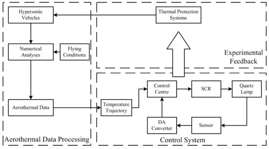
Figure 1.
Flow chart of the TSTQLH system.
In recent years, some control methods have been developed for the TSTQLH, such as fuzzy logic control [18,19] and proportional-integral-derivative (PID) control [20,21,22]. In [18], the transient aerodynamic heating flow of a flying missile body was assessed using a QLH by the fuzzy control method with a complex membership function. In [23], an aerodynamic heating transient test system with a QLH was designed to track real-time heat flux and temperature from a hypersonic vehicle’s trajectory. During the entire control process, fuzzy PID was adopted in a vacuum chamber as the test environment for the TPS. However, fuzzy logic control [24] is mostly based on empirical formulae without a system dynamic model, and its controller cannot achieve a balance between control precision and decision-making effectively. In addition, PID control depends on simply linear superposition of tracking errors and has some errors related to rapidity and overshoot [25]. At the same time, the TSTQLH is process monitoring and some parts of its control system may be out of control due resistance [26], leading to an adverse effect on control capability. Moreover, the TSTQLH control system contains internal uncertainties and external disturbances, causing indeterminacy.
To solve the above-mentioned problems, model-free control (MFC) [27,28,29] is required. For a single input single output (SISO) system, MFC primarily depends on the linear relationship between input and output, along with an ultra-local model. MFC does not rely on the system dynamic model heavily, reducing system complexity and compensating for dynamic disturbances. In general, MFC has four parts: an ultra-local model, a closed-loop controller, an observer, and an auxiliary controller. In [26], an intelligent proportional-integral sliding mode control (iPISMC) was used to track the direct power of the doubly fed induction generator (DFIG). The proposed iPISMC consisted of an iPI (a closed-loop controller) and SMC (an auxiliary controller) in terms of an ultra-local model, along with an extended state observer (ESO, an observer). Under stochastic wind turbulences and parametric uncertainties, the proposed iPISMC was more robust than other classical PIs and iPIs. However, because of the linear superposition of tracking errors, there were some problems related to rapidity and overshoot. In [30], a model-free fractional-order nonsingular fast terminal sliding mode control (MFF-TSMC) was proposed to track the robotic trajectory of a lower-limb robotic exoskeleton. Due to the proposed MFF-TSMC, high precision tracking, fast finite-time convergence, singularity-free and chattering-free operation could be simultaneously ensured in the whole control process. At the same time, because of lack of an auxiliary controller, some errors from the time delay observer and measurement noise still occurred.
Sliding mode control (SMC) [31], as a variable structure control, is robust for system uncertainties and unknown disturbances because of its two distinct states: the switching phase and sliding phase. Before the system state is constrained to lie in a prescribed sliding mode surface, the system state is driven toward the sliding mode surface by the reaching law. During the reaching phase, the system dynamic performance is sensitive to system uncertainties and unknown disturbances resulting from high-frequency switching motions. Moreover, in traditional SMC, the convergence of the system state is asymptotic rather than in finite time. Therefore, some scholars have proposed a terminal SMC, a global SMC, a fractional-order SMC and other SMCs. In [31], a nonsingular terminal SMC was applied for rigid manipulators and the time from any initial state to the equilibrium state was guaranteed to be in finite time. However, some uncertainties sometimes occur in the high frequent switching phase. In [32], a global nonlinear integral SMC associated with a decay function was designed for chaotic synchronization systems to achieve non-integral saturation, fast response and insensitivity to uncertain parameters and disturbances; however, the tracking errors could not converge to zero in finite time.
Neural network control (NNC), as a branch of intelligent control, has the ability of proximation, as in a Hermite neural network (HNN) [33], a layer recurrent neural network (LRNN) [34], an extreme learning machine (ELM) [35], and a radial basis function neural network (RBFNN) [36]. The authors of [33], compared a conventional super-twisting algorithm-based second-order sliding-mode control strategy (STA-SOSM) with a novel HNN-based SOSM control strategy that was found to be more feasible and superior for a synchronous reluctance motor (SynRM) drive system. In [34], the authors used a super-twisting method with artificial neural networks (STA-ANN) for piezoelectric actuators (PEA) to solve nonlinear hysteresis positioning problem. In [35], a fast nonsingular terminal SMC (FNTSMC) combined with an ELM was used with permanent-magnet linear motor systems. Because of FNTSMC and ELM, finite-time convergence, strong control robustness and system dynamics information independence are guaranteed. In [36], a model-free and an NNC based on a time-delay estimator (TDE-MFNNC) was presented for five DOFs in a lower extremity exoskeleton. Compared to a PD controller, NNC and model-free iPD controller, the TDE-MFNNC is more stable and more effective. The RBFNN has a simple structure, faster convergence and better approximation properties, which can be considered as compensators.
This paper proposes a dynamic model of a TSTQLH based on energy conservation and a strategy for an adaptive neural network global nonsingular fast terminal sliding mode model-free control based on a linear extended state observer (ANN-GNFTSMMFC-LESO). The TSTQLH is based on infrared radiation heating of quartz lamp heaters and provides a heating environment by thermal radiation. In terms of the nonlinearity of the control process, the control loop is closed by a global nonsingular fast terminal sliding mode controller (GNFTSMC) instead of an intelligent proportional-integral-derivative (iPID) [26,28] controller because of problems related to rapidity and overshoot. On the basis of the traditional integral sliding mode control, the GNFTSMC eliminates the high-frequency switching phase [32,37] to suppress chattering phenomena and anchors the initial state on the sliding phase to enhance insensitive dynamic performance for internal uncertainties and external disturbances. Moreover, the GNFTSMC introduces a linear term and a nonsingular exponential term into the traditional integral sliding mode control to avoid the singular problem and improves the convergence rate to the equilibrium state in finite time rather than asymptotic convergence [30,31,38]. The LESO is chosen as an observer of the GNFTSMC to estimate internal uncertainties and external disturbances. In addition, an ANN [33,34,35,36] shows good approximation properties in compensation for estimation errors by using a cubic B-spline function [36,39,40]. In the NNC, the cubic B-spline function, as a basis function, has a similar shape to a Gaussian function with the same center positions, and has less inverse multiquadratic functions in terms of computational load. Moreover, the cubic B-spline function, as a piecewise cubic polynomial nonlinear function, has second-order smoothness, which is enough for continuous modeling.
In summary, this paper makes the following contributions:
- (1)
- For hypersonic vehicles, real time ground simulation of aerodynamic heating is established and a thermal-structural test is devised based on an infrared radiation heating platform usinf quartz lamp heaters.
- (2)
- By energy conservation, we establish a dynamic model of TSTQLH. In terms of TSTQLH system dynamic information, the control process of radiation heating, including internal uncertainties and external disturbances, is analyzed.
- (3)
- ANN-GNFTSMMFC-LESO can provide an ultra-local model which can alleviate the dependence of system dynamics. Instead of an iPID controller, the GNFTSMC eliminates the high-frequency switching phase to suppress chattering phenomena, and combines a inear term with a nonsingular exponential term to avoid slow convergence rate and singularity.
- (4)
- We chose a LESO for estimation of lumped disturbances and used a cubic B-spline function in the ANN for observation error compensation with low computational load and second-order smoothness.
- (5)
- The fitting curve wall temperature expression (tracking reference temperature trajectory) of the surface contour from an X-43A wing in a time sequence was obtained by the finite element simulation. The superiority of our proposed control method is validated through comparative simulation results.
2. TSTQLH Control System Modeling
In this section, the mathematical model of the TSTQLH control system is introduced. The TSTQLH control system mainly consists of three parts: a power regulator, QLH, and a temperature sensor. A shown in Figure 2, the power regulator achieves different power values by changing the conduction angle in the AC voltage regulating circuit. Because the power supply is a sinusoidal alternating current; the input electrical energy is converted into thermal energy in the QLH and the QLH provides the thermal environment for untested hypersonic vehicles. The thermocouple acquires temperature data from the QLH and these data are sent to the central controller. As a whole, the controller provides control input of the conduction angle through tracking error to achieve temperature feedback control.
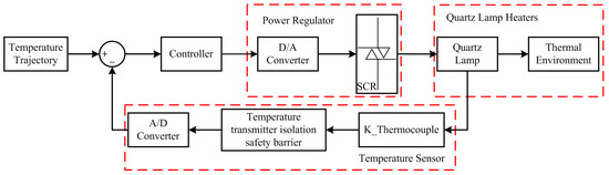
Figure 2.
Flow chart of the TSTQLH control system.
2.1. Electrical Energy
In the power regulator part, the AC voltage regulating circuit can adjust its output power by changing the conduction angle. The expression of the output voltage in the AC voltage regulating circuit is calculated by:
where is the output voltage (V), which is also the input voltage of QLH; is the input supply voltage (V), and is the conduction angle of bidirectional thyristor (rad).
According to Ohm’s law, the input current of QLH can be calculated by:
where is the input current of QLH (A), and is the total resistance of QLH ().
According to the electric power equation, (1) times (2), can be obtained by:
where is the input electric power of QLH (W).
According to Joule’s law, electrical energy absorbed by QLH is expressed as:
where is electric energy acted on QLH () and is the heating time of QLH (s). As a consequence, we establish a mathematical relationship between the conduction angle () of the bidirectional thyristor and electrical energy () absorbed by QLH.
2.2. Thermal Energy
Electric heating energy produced by QLH [41] is deduced by:
where is the electric heating energy (J) produced by the quartz lamp filament, and the first term on the right of (5) represents internal energy consumed by itself. and are the specific heat capacity () and the mass () of the quartz lamp filament, respectively. and are the current temperature (K) and the previous temperature of the time interval (K), respectively. The second term refers to heat transfer in the process of heat convection, heat conduction, and heat radiation. is the surface area () of the QLH tube. is the heat convection coefficient () and is the heat conduction coefficient (). is the blackness coefficient of the quartz lamp filament and is Stephen Boltzmann’s constant (). is the angle coefficient.
2.3. Energy Conservation
According to the law of energy conservation, the energy conservation equation can be defined as:
Substituting (4) and (5) to (6), the equation can be written as:
Then, both sides of (7) are divided by , and the mathematical model of the TSTQLH control system can be given as:
where is the time derivative of . Eventually, a mathematical model between input and output is attained that comprises controllable , a single input variable and measurable , and a single output variable in the TSTQLH control system. Some details are explained in Appendix A.
3. Control Strategy of TSTQLH
The mathematical model of the TSTQLH is a nonlinear and strong coupling system. To ensure great dynamic performances, an ANN-GNFTSMMFC-LESO was developed, as illustrated in Figure 3.
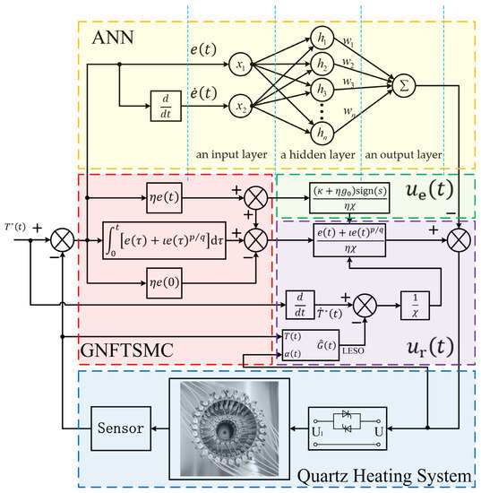
Figure 3.
Schematic illustration for the ANN-GNFTSMMFC-LESO.
In the ANN-GNFTSMMFC-LESO, MFC, GNFTSMC, LESO, and ANN are combined to form a closed loop. MFC uses an ultra-local model to linearize the TSTQLH control system mathematical model. The GNFTSMC anchors the initial system state on the sliding phase and is insensitive to internal uncertainties and external disturbances, suppressing chattering phenomena caused by the high-frequency switching phase. In addition, the LESO and the ANN are the disturbances observer and the observation error compensator, respectively. The ANN has an effective approximation property with low computational load and second-order smoothness attained by using a cubic B-spline function.
3.1. Model-Free Control
For the SISO system, the basic principle of MFC [28] is an ultra-local model, which primarily depends on the input-output behavior.
Equation (8) can be rewritten as:
The mathematical model of the TSTQLH is transformed into an ultra-local model, defined as:
where is the sum of unknown terms including internal uncertainties and external disturbances from local periodic oscillation () and high-order nonlinear output (), is a non-physical constant parameter which is achieved by experiments, and is the input variable.
3.2. LESO
The most vital point of the MFC is to gain the value of the unknown terms exactly and timely. Considering that there are some internal uncertainties and external disturbances existed in the TSTQLH control system, LESO is chosen as an observer:
where , is the observation value of , is the observation value of ; ; and are the gain parameters.
The observation error is defined as:
where is the observation error and satisfies the condition . is an upper bound value, and is the observation value and is equal to ;
3.3. GNFTSMMFC-LESO
Define:
where is the tracking error, and is reference temperature trajectory.
Then, both sides of (14) are divided by :
Substituting (10) and (13) to (15), can be written as:
In order to establish the closed-loop controller, the GNFTSMC is defined as:
where . These are the coefficients of the fast term and the nonsingular term, respectively, and ensures second-order nonsingularity and are positive odd integers. is the initial state of the tracking error. It is obvious that the GNFTSMC anchors the initial system state on the sliding phase and its system state is trapped on the sliding phase without disturbances interference, i.e., .
The derivative of (17) is:
Then, via (18), the finite time of convergence to equilibrium state is calculated:
Calculation of (19) is given in Appendix B in detail.
Define:
where is the input of GNFTSMC, and and are equivalent control law and reaching control law, respectively.
Substituting (16) and to (18), is calculated as:
Sometimes, and may occur leading to convergence stagnation, and the reaching control law is necessary.
The accessibility condition of GNFTSMC is:
where is a positive integer.
Substituting (18) to (22), Equation (22) can be written:
Substituting (16) to (23), Equation (23) can be written:
During the GNFTSMMFC-LESO controller, is equal to to obtain the reaching control law . Substituting (20) to (24), Equation (24) can be written:
Substituting (21) to (25), Equation (25) can be written:
Let be equal to its maximum value , , then:
Then, is:
3.4. ANN-GNFTSMMFC-LESO
In GNFTSMMFC-LESO, substituting (28) to (10), the error function is calculated:
Let , then Equation (29) is rewritten:
In practical applications, Equation (30) reveals that the measurement noise and the inadequate GNFTSMMFC-LESO are inevitable. Therefore, the lumped unknown disturbances need some online improvements by adding an auxiliary controller.
In this part, a neural network controller, as an auxiliary controller, is an online compensator for the lumped unknown disturbances . In general, a neural network controller consists of three parts: an input layer, a hidden layer and an output layer.
Define:
where is the optimal weight and satisfies , is a hidden layer function, which is a piecewise form, and is the approximate error.
By contrast with two main hidden layer functions [36,40]: Gaussian function () and Inverse multiquadratic function (), the cubic B-spline function is defined thus:
where is the Euclidean norm and is the basis function center positions, is the input of the ANN controller, and is the width. In neural network control, the cubic B-spline function [42], as basis function, has a similar shape to the Gaussian function with the same center positions, and is less than the inverse multiquadratic functions in terms of computational load. Moreover, the cubic B-spline function, as a piecewise cubic polynomial nonlinear function, has second-order smoothness, which is enough for continuous modeling. This satisfies these conditions:
where , are positive integers, respectively, and, in this paper, .
Define the ANN-GNFTSMMFC-LESO controller:
where is the input of the ANN controller.
Substituting (36) to (10), then (36) is calculated:
Substituting (28) to (37), then (37) is calculated:
Substituting (31) to (38), then (38) is calculated:
where the ANN controller is an online compensator for the , along with . satisfies the condition:
where is the estimation value of , is the adaptive law of , and is the gain parameter of the adaptive law.
Eventually, the ANN-GNFTSMMFC-LESO controller is obtained:
3.5. Stability Analysis
Proof.
Stability of LESO is proven. □
Theorem 1.
For a linear system, which;;;; if it satisfies that the eigenvalues of a matrixare less than zero, this linear system is stable.
Proof of Theorem 1.
Equation (12) is rewritten:
where , , . By calculation, the eigenvalues of a matrix ( and ) satisfy these conditions:
where the eigenvalues of a matrix ( and ) are less than zero and the LESO is stable. □
Proof.
The stability of the ANN-GNFTSMMFC-LESO controller is proven. □
Define the Lyapunov function:
where is the weight error and ; .
The derivative of (45) is:
Then, substituting (18) to (46), (46) is calculated:
Then, substituting (16) to (47), (47) is calculated:
Then, substituting (42) to (48), (48) is calculated:
Then, substituting (31) to (49), (49) is calculated:
where, if (50) satisfies , , then the . The ANN-GNFTSMMFC-LESO controller is stable.
Proof.
Proof of the ANN-GNFTSMMFC-LESO controller is bounded in finite time:
When (50) satisfies, (50) is calculated:
Then, (51) is calculated:
□
Theorem 2 [43,44].
The inequality satisfies:
where,,andis a positive integer.
Theorem 3.
Consider the system. Define:
where,,and.
Then, the trajectory of the closed-loop system is bounded in finite time:
where. The finite time which is needed to reach the (51) is bounded:
whereis the initial value of.
According to Theorem 2, (53) is calculated:
According to Theorem 3 and (59), the finite time is calculated:
where the system state converges to (60) in the finite time (61).
4. Aerothermal Data Processing
In this section, the temperature trajectory, a tracking goal of the TSTQLH control system, is confirmed by finite element simulation using ANSYS Workbench 2020 R2. Therefore, the type of a hypersonic vehicle and its flight parameters, such as flight trajectory and the corresponding atmospheric environment, are necessary.
4.1. Flight Trajectory of Hypersonic Vehicles and the Corresponding Atmospheric Envirooment
Figure 4 shows the flight trajectory of X-43A. The flight process consists of about three stacks of a B-52B aircraft, a booster rocket and X-43A. At the beginning, a booster rocket and X-43A are carried by a B-52B aircraft to the Pacific at 40,000 feet altitude. A booster rocket and the X-43A are separated from the B-52B aircraft and a booster rocket lifts X-43A. Finally, at about 9500 feet, a scramjet engine starts to operate and the X-43A continues to fly for about ten seconds. As a result, the type of a hypersonic vehicle and its fight trajectory are identifies as the finite element simulation’s object. In addition, the flight trajectory of the X-43A is divided into 31 different groups, including subsonic velocity, transonic velocity, supersonic velocity and hypersonic velocity, and the corresponding atmospheric environment is calculated via the ATMOSCOESA (H) function in Table 1. The committee on extension to the Standard Atmosphere has the acronym COESA. The ATMOSCOESA (H) function implements a mathematical representation of the 1976 COESA United States standard lower atmospheric values. H, T, a, P and R are the altitude (m), the temperature (K), the sound velocity (m/s), the pressure (Pa) and the density (kg/m3) of the corresponding atmospheric environment, and M is the X-43A flight speed (Mach number). For example, if we calculate the COESA model at 12,192 m in MATLAB with ATMOSCOESA input (12,192), results are obtained.
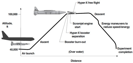
Figure 4.
Flight trajectory of the X-43A [45].

Table 1.
The corresponding atmospheric environment.
4.2. Finite Element Simulation Results
According to Table 1, the surface contour of an X-43A wing is chosen as the wall in the external flow field (Figure 4 red line), and the 31 different groups with four types of wedged angles (45°, 30°, 15°, 20°) are calculated in the finite element simulation, in which 45° connects to group a, 30° connects to groups b~k, 15° connects to groups l~A, and 20° connects to groups B~E. As is shown in Figure 5, the left, right and top of each of two-dimension external flow fields are the set inlet, outlet, and pressure-far-field, respectively, with different boundary conditions, corresponding to the Table 1.
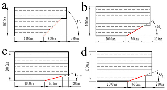
Figure 5.
The external flow field with four types of wedged angles (a) 45°, (b) 30°, (c) 15°, (d) 20°. The red line is the wall of the surface contour from a X-43A wing.
Each two-dimension external flow field uses the triangles method to generate Mesh with different element qualities of the Mesh Metric in Table 2.
Table 2.
Different element quality of the Mesh Metric.
These 31 groups of 45°, 30°, 15°, 20° wedged angles are associated with different solutions of the calculation in Table 3 and Table 4. The initialization method takes hybrid initialization with 15 iterations in the calculation. Based on the above-mentioned setting parameters, the finite element simulation results are shown in Figure 6.
Table 3.
Different solutions in detail.
Table 4.
Different solution controls in detail.
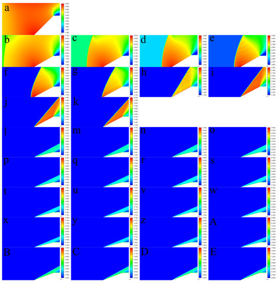
Figure 6.
Finite element simulation results and the 31 different figures with four types of wedged angles (45°, 30°, 15°, 20°) are calculated in the finite element simulation, in which 45° connects to (a), 30° connects to (b–k), 15° connects to (l–A), and 20° connects to (B–E).
Based on the finite element simulation results, the wall temperature values of the surface contour of a X-43A wing (the red line in Figure 5) are chosen to plot scatter graphs concerning position and temperature relationships, as shown in Figure 7. From Figure 7, it is obvious that the link between the rising temperature and the X-43A flight speed is a positive correlation. Each group is an independent time interval, and the maximum wall values from each scatter graph of different positions are plotted as a scatter graph in Figure 7e. In Figure 7e, the fitting curve wall temperature expression of the surface contour from a X-43A wing in a time sequence is as follows:
where is the temperature trajectory of the TSTQLH control system, is the flight time, and SSE, R-square, Adjusted R-square and RMSE are equal to 4444, 0.9988, 0.9984 and 14.21, respectively.
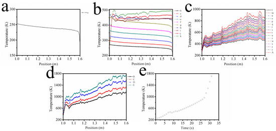
Figure 7.
(a–d) Scatter graphs showing position and temperature relationships, and (e) the temperature trajectory curve.
Remark.
The QLH is a kind of tungsten filament quartz lamp. To obtain proper parameters of the ANN-GNFTSMMFC-LESO controller, some steps are applied. The sampling period of the simulation test is 31 s in MATLAB 2014b.
- Step 1:
- Tuneby increasing its values from negative to positive until the control trend declines, when other parameters are equal to 0.
- Step 2:
- If step 1 is unsuccessful, tuneandfrom small to large by satisfying,until the control trend declines, when other parameters still maintain 0.
- Step 3:
- Maintain the values of,,, tune,, andby satisfying, , andwhile checking the tracking error and chattering.
- Step 4:
- Maintain the values of,,,,, and, tuneandby satisfyingand positive odd integers while checking the tracking error and chattering.
- Step 5:
- Finally, tuneandcorresponding to the tracking error while checking the tracking error and chattering. In addition, during other controllers, the same parameters are the same as in the proposed controller (ANN-GNFTSMMFC-LESO controller). Other parameters are set by the above-mentioned tuning procedures.
5. Simulation Results
Under optimized conditions, the ANN-GNFTSMMFC-LESO controller was further studied based on the TSTQLH. The parameters of QLH are listed as: ; ;; ; ; ; ; ; ; . The parameters of the ANN-GNFTSMMFC-LESO controller are listed as: ; ; ; ;; ; ;; ; ; ;
, ; ; . Other parameters are the same. All parameters are shown in Table 5, Table 6, Table 7, Table 8, Table 9 and Table 10.
Table 5.
Some parameters of the QLH.
Table 6.
Parameters of the ANN-GNFTSMMFC-LESO controller.
Table 7.
Parameters of the GNFTSMMFC-LESO controller.
Table 8.
Parameters of the TSMFC-LESO controller.
Table 9.
Parameters of the iPIDMFC controller.
Table 10.
Parameters of the PID controller.
As is shown in Figure 8 and Figure 9, there are other four comparative control strategies, including the GNFTSMMFC-LESO controller, the TSMFC-LESO controller, iPIDMFC controller, and the PID controller. The GNFTSMMFC-LESO controller has the same sliding mode surface and LESO as the proposed scheme (ANN-GNFTSMMFC-LESO controller) with the auxiliary controller ANN. The TSMFC-LESO controller has a traditional TSM surface (). The iPIDMFC controller combines the PID controller with the MFC, which is defined as:
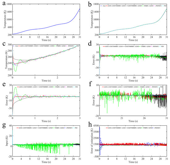
Figure 8.
Simulation results without extra disturbances. (a) Fitting curve temperature trajectory. (b) Tracking temperature trajectory, and (c) partially enlarged figure details. (d) Tracking error and (e,f) partially enlarged figure details. (g) Input of some controllers. (h) Estimation error of some controllers.
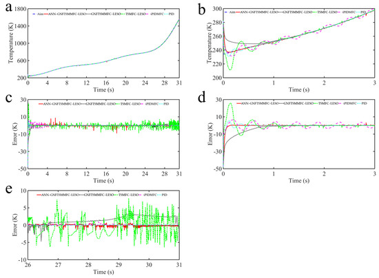
Figure 9.
Simulation results with extra disturbances. (a) Tracking temperature trajectory and (b) partially enlarged figure details. (c) Tracking error and (d,e) partially enlarged figure details.
As shown in Figure 8a (the reference temperature trajectory of Equation (62)) and Figure 8, the fitting curve wall temperature of the surface contour from an X-43A wing in time sequence is chosen as a reference trajectory, which is from 234.2 k in 0 s to 1711.79 k in 31 s. From Figure 8b,c, these controllers have a silimar trend about the tracking dynamic performances. At the beginning, from 1.0 s to 3.0 s, the ANN-GNFTSMMFC-LESO controller has the shortest response time and other cotrollers have overshoot phenomena with different levels. From Figure 8d,e, chattering phenomena occur in the TSMFC-LESO controller because of the traditional TSM surface with a high-frequency switching phase during the whole process. In Figure 8f, chattering phenomena occur in the GNFTSMMFC-LESO controller at a later time from 24 s to 31 s, due to the lack of the auxiliary controller ANN, leading to estimation error accumulation. In Figure 8g,h, it is apparent that the ANN-GNFTSMMFC-LESO controller has the smallest input and estimation error due to the combined effects of MFC, GNFTSMC and ANN.
Considering the QLH as an infrared radiation heating element, its resistance is sensitive to its temperature. The time-varying resistance of the quartz lamp filament is selected as a disturbance and its equation is:
Figure 9 reveals that the time-varying resistance has an adverse impact on performances which enlarges the fluctuation range and prolongs stabilization time. By contrast, the ANN-GNFTSMMFC-LESO controller has robustness to some disturbances. According to Figure 9c,d, the tracking error of the ANN-GNFTSMMFC-LESO controller decreases dramatically at the beginning, then remains stable until 31 s. By contrast, the largest fluctuation occurred in the tracking error of the TSMFC-LESO controller at around 30 k at 0.2 s and reached a relative steady state at 3.0 s. However, at the later stage of the control process, the TSMMFC-LESO controller had more chattering as shown in Figure 9e. The GNFTSMMFC-LESO controller had a steady state error because of the lack of the auxiliary controller ANN. If the time-varying resistance occurred, there were some tracking fluctuations for iPIDMFC controller and PID controller. In fact, the PID is based on output error feedback to eliminate error and its final state may be stable. However, the real output is an inertial variable without any sudden changes. Some nonlinear, unknown features and external uncertainties are involved in this control system, which cause sudden changes in the control process. This means that the non-jumping variable is used to control the jumping variable, leading to a conflict between rapidity and overshoot.
To make quantitative comparisons, calculations of simulation results from 10 s to 20 s are given in Table 11, including the root mean square error , the Maximum error .
Table 11.
Calculations of RMSe and Max.
The above results show that the ANN-GNFTSMMFC-LESO controller possesses strong robustness in tracking temperature trajectory and its tracking error can rapidly converge to zero. Internal system parameters make no significant difference on its tracking precision over the period from 0 s to 31 s. Compared with GNFTSMMFC-LESO controller, TSMFC-LESO controller, iPIDMFC controller, and PID controller, the ANN-GNFTSMMFC-LESO control strategy has great application in real time ground simulation of aerodynamic heating produced by hypersonic vehicles.
6. Conclusions
In summary, the TSTQLH was established as a real time ground simulation system of aerodynamic heating for the examination of the hypersonic vehicle TPS, along with control system analyses. Due to a lack of system dynamic information, previous control methods such as fuzzy control and PID control have some deficiencies, which are sensitive to system parameter uncertainties and external disturbances. This paper proposes an ANN-GNFTSMMFC-LESO controller that contains three parts: an MFC with LESO, a GNFTSMMFC controller, and an auxiliary controller ANN. The MFC improves performance of the controlled object with nonlinearity, high-order terms and dynamic disturbances to alleviate the dependence of system dynamics. The GNFTSMMFC controller has a new sliding mode surface without a high-frequency switching phase to suppress chattering phenomena, and the initial system state is trapped on the sliding mode being insensitive to lumped disturbances. Therefore, fast response, strong robustness, and finite-time convergence are simultaneously guaranteed. The ANN, as an estimation error compensator, uses a cubic B-spline function with low computational load and second-order smoothness, and has the ability of eliminating extra disturbances for system dynamic performance. The temperature trajectory of the surface contour from an X-43A wing in a time sequence was calculated by finite element simulation (ANSYS Workbench 2020 R2) with 31 different groups and its fitting curve was chosen as a tracking target. Under optimized conditions, the proposed ANN-GNFTSMMFC-LESO controller was validated to successfully track temperature trajectory during simulation demonstrations (MATLAB 2014b).
Author Contributions
Conceptualization, X.L.; methodology, X.L.; software, M.Z.; validation, M.Z., Z.S. and Z.B.; formal analysis, X.L.; data curation, X.L.; writing—original draft preparation, X.L.; writing—review and editing, H.O.; visualization, H.O.; supervision, I.V.A.; project administration, G.Z.; funding acquisition, G.Z. All authors have read and agreed to the published version of the manuscript.
Funding
This research was funded by China Scholarship Council (No. 202108670007).
Institutional Review Board Statement
Not applicable.
Informed Consent Statement
Not applicable.
Data Availability Statement
Not applicable.
Acknowledgments
The authors would like to express their gratitude to all those who helped them during the writing of this paper.
Conflicts of Interest
The authors declare no conflict of interest.
Appendix A
Theorem A1.
In mathematics, a real variable is differentiable at a pointof its domain. If the limitexists, it is:
So, this limit is called the derivative of a real variableat a point, denotedor.
According to Theorem 4, the calculation process of (8) is:
Based on (7), both sides are divided by and further calculated by:
where the control process of TSTQLH always tracks the reference temperature trajectory. In particular, is the current temperature (K) and is the previous temperature of the time interval (K).
Then, the derivative of is calculated by:
where the limit exists and , is equal to the limit.
Then, (8) is obtained by:
Appendix B
The calculation process of (19) is:
Let :, then (A5) is rewritten as:
Because of a first order differential equation, (A7) is calculated as:
where, is an arbitrarily constant.
Then, substituting to (A8), (A8) is calculated:
Therefore, the finite time of convergence to equilibrium state is:
where are steady-state errors.
References
- Urzay, J. Supersonic Combustion in Air-Breathing Propulsion Systems for Hypersonic Flight. In Annual Review of Fluid Mechanics; Davis, S.H., Moin, P., Eds.; Annual Reviews: Palo Alto, CA, USA, 2018; Volume 50, pp. 593–627. [Google Scholar]
- Sun, X.; Huang, W.; Ou, M.; Zhang, R.; Li, S. A survey on numerical simulations of drag and heat reduction mechanism in supersonic/hypersonic flows. Chin. J. Aeronaut. 2019, 32, 771–784. [Google Scholar] [CrossRef]
- Zhang, T.-T.; Wang, Z.-G.; Huang, W.; Chen, J.; Sun, M.-B. The overall layout of rocket-based combined-cycle engines: A review. J. Zhejiang Univ. Sci. A 2019, 20, 163–183. [Google Scholar] [CrossRef]
- Han, C.; Bai, S.; Sun, X.; Rao, Y. Hovering Formation Control Based on Two-Stage Constant Thrust. J. Guid. Control. Dyn. 2020, 43, 504–517. [Google Scholar] [CrossRef]
- Levchenko, I.; Xu, S.; Teel, G.; Mariotti, D.; Walker, M.L.R.; Keidar, M. Recent progress and perspectives of space electric propulsion systems based on smart nanomaterials. Nat. Commun. 2018, 9, 879. [Google Scholar] [CrossRef]
- Yang, C.; Zhao, H.; Wu, Z. Research progress of aerothermoelasticity of air-breathing hypersonic vehicles. J. Beijing Univ. Aeronaut. Astronaut. 2019, 45, 1911–1923. [Google Scholar]
- Huang, D.; Friedmann, P.P.; Rokita, T. Aerothermoelastic Scaling Laws for Hypersonic Skin Panel Configurations with Arbitrary Flow Orientation. AIAA J. 2019, 57, 4377–4392. [Google Scholar] [CrossRef]
- Jiang, G.; Li, F. Aerothermoelastic analysis of composite laminated trapezoidal panels in supersonic airflow. Compos. Struct. 2018, 200, 313–327. [Google Scholar] [CrossRef]
- Kumar, S.; Mahulikar, S.P. Aero-thermal analysis of lifting body configurations in hypersonic flow. Acta Astronaut. 2016, 126, 382–394. [Google Scholar] [CrossRef]
- Gong, C.-L.; Gou, J.-J.; Hu, J.-X.; Gao, F. A novel TE-material based thermal protection structure and its performance evaluation for hypersonic flight vehicles. Aerosp. Sci. Technol. 2018, 77, 458–470. [Google Scholar] [CrossRef]
- Wang, J.-F.; Li, J.-W.; Zhao, F.-M.; Fan, X.-F. Numerical method of carbon-based material ablation effects on aero-heating for half-sphere. Mod. Phys. Lett. B 2018, 32, 1840011. [Google Scholar] [CrossRef]
- Sivamurugan, T.; Anoop, P.; Desikan, S.L.N. Aerothermal design, qualification and flight performance. Curr. Sci. 2018, 114, 64–67. [Google Scholar] [CrossRef]
- Meng, S.; Yang, Q.; Xie, W.; Xu, C.; Jin, H. Comparative Study of Structural Efficiencies of Typical Thermal Protection Concepts. AIAA J. 2017, 55, 2476–2480. [Google Scholar] [CrossRef]
- Yu, K.; Xu, J.; Liu, S.; Zhang, X. Starting characteristics and phenomenon of a supersonic wind tunnel coupled with inlet model. Aerosp. Sci. Technol. 2018, 77, 626–637. [Google Scholar] [CrossRef]
- Zhu, Y.; Zeng, L.; Dong, W.; Du, Y.; Gui, Y. Computational and Experimental Study on Quartz Lamp Array Heat Flux Distribution. J. Astronaut. 2017, 38, 1131–1138. [Google Scholar]
- Zhu, Y.; Wei, D.; Liu, S.; Zeng, L.; Gui, Y. Power optimization of non-uniform aerodynamic heating simulated by quartz lamp array. Acta Aeronaut. Et Astronaut. Sin. 2019, 40, 122761. [Google Scholar]
- Zhu, Y.; Liu, X.; Zeng, L.; Gui, Y. Comparison Research of Methods for Quartz Lamp Heat Flux Simulation. J. Eng. Thermophys. 2019, 40, 1397–1402. [Google Scholar]
- Wu, D.; Gao, Z.; Wang, Y. Experimental Study on Fuzzy Control of Transient Aerodynamic Heat Flow of Missile. J. Beijing Univ. Aeronaut. Astronaut. 2002, 28, 682–684. [Google Scholar]
- Shen, Q.; Shi, Y.; Jia, R.; Shi, P. Design on Type-2 Fuzzy-Based Distributed Supervisory Control With Backlash-Like Hysteresis. IEEE Trans. Fuzzy Syst. 2021, 29, 252–261. [Google Scholar] [CrossRef]
- Gao, P.; Zhang, G.; Ouyang, H.; Mei, L. An Adaptive Super Twisting Nonlinear Fractional Order PID Sliding Mode Control of Permanent Magnet Synchronous Motor Speed Regulation System Based on Extended State Observer. IEEE Access 2020, 8, 53498–53510. [Google Scholar] [CrossRef]
- Luo, W.; Khoo, Y.S.; Hacke, P.; Naumann, V.; Lausch, D.; Harvey, S.P.; Singh, J.P.; Chai, J.; Wang, Y.; Aberle, A.G.; et al. Potential-induced degradation in photovoltaic modules: A critical review. Energy Environ. Sci. 2017, 10, 43–68. [Google Scholar] [CrossRef] [Green Version]
- Zhao, D.; Wang, Z.; Ding, D.; Wei, G. H-infinity PID Control With Fading Measurements: The Output-Feedback Case. IEEE Trans. Syst. Man Cybern. Syst. 2020, 50, 2170–2180. [Google Scholar] [CrossRef]
- Yu-zhu, H.O.U.; Jing-liang, Z.; Wei, D. Transient test of aerodynamic heating for hypersonic vehicle. J. Aerosp. Power 2010, 25, 343–347. [Google Scholar]
- Castillo, O.; Amador-Angulo, L.; Castro, J.R.; Garcia-Valdez, M. A comparative study of type-1 fuzzy logic systems, interval type-2 fuzzy logic systems and generalized type-2 fuzzy logic systems in control problems. Inf. Sci. 2016, 354, 257–274. [Google Scholar] [CrossRef]
- Song, J.; Wang, L.; Cai, C.; Qi, X. Nonlinear fractional order proportion-integral-derivative active disturbance rejection control method design for hypersonic vehicle attitude control. Acta Astronaut. 2015, 111, 160–169. [Google Scholar] [CrossRef]
- Li, S.; Wang, H.; Tian, Y.; Aitouch, A.; Klein, J. Direct power control of DFIG wind turbine systems based on an intelligent proportional-integral sliding mode control. Isa Trans. 2016, 64, 431–439. [Google Scholar] [CrossRef] [PubMed]
- Lee, S.W.; Shimojo, S.; O’Doherty, J.P. Neural Computations Underlying Arbitration between Model-Based and Model-free Learning. Neuron 2014, 81, 687–699. [Google Scholar] [CrossRef] [Green Version]
- Fliess, M.; Join, C. Model-free control. Int. J. Control. 2013, 86, 2228–2252. [Google Scholar] [CrossRef] [Green Version]
- Hou, Z.; Jin, S. Data-Driven Model-Free Adaptive Control for a Class of MIMO Nonlinear Discrete-Time Systems. IEEE Trans. Neural Netw. 2011, 22, 2173–2188. [Google Scholar] [CrossRef]
- Ahmed, S.; Wang, H.; Tian, Y. Model-free control using time delay estimation and fractional-order nonsingular fast terminal sliding mode for uncertain lower-limb exoskeleton. J. Vib. Control. 2018, 24, 5273–5290. [Google Scholar] [CrossRef]
- Feng, Y.; Yu, X.H.; Man, Z.H. Non-singular terminal sliding mode control of rigid manipulators. Automatica 2002, 38, 2159–2167. [Google Scholar] [CrossRef]
- Xu, G.W.; Zhao, S.D.; Cheng, Y. Chaotic synchronization based on improved global nonlinear integral sliding mode control**. Comput. Electr. Eng. 2021, 96, 107497. [Google Scholar] [CrossRef]
- Liu, Y.-C.; Laghrouche, S.; N’Diaye, A.; Cirrincione, M. Hermite neural network-based second-order sliding-mode control of synchronous reluctance motor drive systems. J. Frankl. Inst. Eng. Appl. Math. 2021, 358, 400–427. [Google Scholar] [CrossRef]
- Napole, C.; Barambones, O.; Derbeli, M.; Calvo, I.; Silaa, M.Y.; Velasco, J. High-Performance Tracking for Piezoelectric Actuators Using Super-Twisting Algorithm Based on Artificial Neural Networks. Mathematics 2021, 9, 244. [Google Scholar] [CrossRef]
- Zhang, J.; Wang, H.; Cao, Z.; Zheng, J.; Yu, M.; Yazdani, A.; Shahnia, F. Fast nonsingular terminal sliding mode control for permanent-magnet linear motor via ELM. Neural Comput. Appl. 2020, 32, 14447–14457. [Google Scholar] [CrossRef]
- Zhang, X.; Wang, H.; Tian, Y.; Peyrodie, L.; Wang, X. Model-free based neural network control with time-delay estimation for lower extremity exoskeleton. Neurocomputing 2018, 272, 178–188. [Google Scholar] [CrossRef]
- Chu, Y.; Fei, J.; Hou, S. Dynamic global proportional integral derivative sliding mode control using radial basis function neural compensator for three-phase active power filter. Trans. Inst. Meas. Control. 2018, 40, 3549–3559. [Google Scholar] [CrossRef]
- Hou, H.; Yu, X.; Xu, L.; Rsetam, K.; Cao, Z. Finite-Time Continuous Terminal Sliding Mode Control of Servo Motor Systems. IEEE Trans. Ind. Electron. 2020, 67, 5647–5656. [Google Scholar] [CrossRef]
- Jiwari, R.; Pandit, S.; Koksal, M.E. A class of numerical algorithms based on cubic trigonometric B-spline functions for numerical simulation of nonlinear parabolic problems. Comput. Appl. Math. 2019, 38. [Google Scholar] [CrossRef]
- Kamath, A.; Manzhos, S. Inverse Multiquadratic Functions as the Basis for the Rectangular Collocation Method to Solve the Vibrational Schrodinger Equation. Mathematics 2018, 6, 253. [Google Scholar] [CrossRef] [Green Version]
- Xia, L.S.; Bin, Q.I.; Tian, N.; Cao, Y.Q.; Hong-Liang, L.I.J.I.T. Study on Modeling Analysis and Testing Method of Electro-thermal Properties of Quartz Lamp. Infrared Technol. 2015, 37, 877–882. [Google Scholar]
- Saranli, A.; Baykal, B. Complexity reduction in radial basis function (RBF) networks by using radial B-spline functions. Neurocomputing 1998, 18, 183–194. [Google Scholar] [CrossRef]
- Zhu, Z.; Xia, Y.; Fu, M. Attitude stabilization of rigid spacecraft with finite-time convergence. Int. J. Robust Nonlinear Control. 2011, 21, 686–702. [Google Scholar] [CrossRef]
- Wang, Y.; Gu, L.; Gao, M.; Zhu, K. Multivariable Output Feedback Adaptive Terminal Sliding Mode Control for Underwater Vehicles. Asian J. Control. 2016, 18, 247–265. [Google Scholar] [CrossRef]
- Zhang, Y.; Chen, L.; Yang, R.; Tu, J. Development and Aero-Heating Tests of Sharp Leading Edge in Hypersonic Vehicles. Aerosp. Mater. Technol. 2012, 42, 1–4. [Google Scholar]
Publisher’s Note: MDPI stays neutral with regard to jurisdictional claims in published maps and institutional affiliations. |
© 2022 by the authors. Licensee MDPI, Basel, Switzerland. This article is an open access article distributed under the terms and conditions of the Creative Commons Attribution (CC BY) license (https://creativecommons.org/licenses/by/4.0/).