Numerical Simulation of Oil Shale Pyrolysis under Microwave Irradiation Based on a Three-Dimensional Porous Medium Multiphysics Field Model

Abstract

The pyrolysis characteristics of oil shale during heat treatment dominate the oil production of kerogen. In this study, the pyrolysis characteristics of oil shale in a laboratory microwave apparatus were investigated based on a novel fully coupled three-dimensional electromagnetic-thermal-chemical-hydraulic model according to the experimental microwave apparatus. By simulating the electric field, temperature distribution, and kerogen decomposition within oil shale subjected to microwave irradiation, several parameters, including waveguide, position, and power, were successfully optimized. The results indicated that the non-uniform temperature distribution was consistent with the distribution of the electric field. Double microwave ports were more effective than single ports in terms of heating rate and temperature uniformity. There was an optimal location where the highest heating efficiency was obtained, which was on the left of the cavity center. When irradiation was conducted over a range of microwave powers, a higher power was suitable for achieving a rapid temperature increase, whereas a lower power was suitable to gain a high efficiency of the pyrolysis rate. Therefore, a variable power heating mode was introduced to decrease the heating time and improve the heat uniformity simultaneously during oil shale pyrolysis. Specifically, the secondary reactions of oil products should be maximally avoided by controlling the microwave power.

1. Introduction

As society and technology develop by leaps and bounds, large amounts of oil and gas are consumed worldwide, and these resources are projected to satisfy up to 55% of the world’s energy demand in 2040 [1,2]. With the decline in light oil reserves, attention has shifted toward unconventional energy sources, such as shale oil and gas, which can contribute to future demands. Oil shale, as an important fossil fuel, is a vital energy replacement for conventional hydrocarbon resources [3,4]. Oil shale is a promising unconventional resource because it can provide almost 400 billion tons of shale oil, which can be extracted from oil shale resources all over the world [5,6,7]. To obtain oil and gas, oil shale needs to be pyrolyzed via heating in order to transform its organic matter—called kerogen—into hydrocarbons [8,9,10].

A variety of experimental research shows the great potential of microwave heating in oil engineering [11,12,13]. Taheri-Shakib et al. [12] conducted an experiment comparing heavy crude oil heated by a microwave heating technique versus the conventional heating technique. The results showed that the microwave heating technique was beneficial in increasing light carbonic components and decreasing the sulfur content in heavy oil. Conventional heating, including electrical heating and steam heating, has been comprehensively investigated for the pyrolysis of oil shale; however, its low heating rate, low transformation efficiency, and high energy consumption cannot be avoided [14,15]. Considering that it has many unique advantages in comparison with conventional heating [16,17,18,19], microwave heating has been proposed for oil shale pyrolysis [20,21,22]. Samer et al. [23] introduced a novel technique to extract shale oil from oil shale and tested several solvents for extractive capacity at different temperatures during the microwave irradiation of oil shale. Ana et al. [24] studied the transformation of an oil shale sample using two different heating strategies: microwave irradiation and conventional heating. They found that the two strategies afforded similar yields of liquid products; however, the overall energy requirements were considerably lower when microwave irradiation was conducted. El Harfi et al. [25] designed a special microwave cavity and reactor to study the pyrolysis of oil shale and concluded that the oil obtained by microwave heating was more maltenic, less polar, and contained lower amounts of sulfur and nitrogen than the oil obtained using conventional technology. Therefore, the microwave heating of oil shale in domestic experiments has tremendous advantages, including low energy consumption and the generation of high-quality oil products.

Laboratory experiments are a direct and credible approach to research microwave heating; however, they cannot accurately reveal the pyrolysis process under microwave heating and thus cannot optimize the heating parameters. Some meaningful data cannot be obtained through physical experiments, including the electromagnetic distribution of the microwave oven and the internal thermal evolution of sample [26,27]. Numerical simulations have increasingly become an auspicious way to visualize and quantify the microwave heating process because of the availability of higher computational power and the development of efficient numerical methods [28,29]. For oil shale pyrolysis, there is a lack of numerical simulations of the microwave heating method. Zhao et al. [30] investigated the promotion of oil shale pyrolysis using heat-carrying supercritical carbon dioxide (SC-CO₂) in laboratory experiments and numerical simulations and obtained the diffusion and velocity distributions of SC-CO₂. Wang et al. [31] identified and investigated the chemical structural parameters of kerogen from Yaojie oil shale and determined a reasonable three-dimensional model of Yaojie kerogen via molecular simulation methods, anneal dynamics simulations, and geometry optimization calculations. Zhu et al. [32] established a mathematical model to investigate the in situ upgrading of oil shale reservoirs and analyzed the effects of microwave power and the thermal conductivity of oil shale. They found that higher power was associated with higher oil and gas production. Furthermore, if the power was too high and the reservoir’s thermal conductivity too low, an underground overheating phenomenon near the wellbore was observed. When applying electromagnetics, the waveguide number and sample position are also important for the heating efficiency. However, few reports are available in the literature that present the effects of the heating parameters on oil shale pyrolysis through microwave heating.

The microwave pyrolysis of oil shale involves the complex coupling of electromagnetics, heat transfer, chemical reactions, and mass transport. To better understand the pyrolysis process, a fundamental model is required to provide quantitative information regarding the most important physical changes and chemical reactions that occur during oil shale pyrolysis. In this study, the simulation results were verified using temperature data obtained from laboratory experiments. In summary, the objectives of this research were to (1) establish and resolve a coupled electromagnetic-thermal-chemical-hydraulic model to investigate the mechanism of oil shale pyrolysis; (2) validate the model by grid-independent tests and laboratory experiments; (3) optimize the heating parameters, including waveguide, sample position, and microwave power; and (4) analyze the mass transfer of oil and gas products within oil shale based on the optimal parameters for microwave irradiation.

2. Governing Equations

The pyrolysis of oil shale under microwave irradiation involves electromagnetic wave excitation, heat transfer in porous media, chemical reactions, mass transfer, and product flow; thus, the governing equations include Maxwell’s equations, the energy conservation equation, the chemical reaction rate equation, the mass conservation equation, and the Brinkman equations. The coupling relationship among these equations is shown in Figure 1.

2.1. Electromagnetic Wave Excitation

Electromagnetic analysis at a macroscopic level involves solving Maxwell’s equations, which are subject to certain boundary conditions. For general time-varying fields, Maxwell’s equations can be written as follows:

$$\nabla \times {\mu }_r^{-1}(\nabla \times \mathit{E})-{\mathrm{k}}_0^2({\epsilon }_r-\frac{j\sigma }{\omega {\epsilon }_0})\mathit{E}=0$$

(1)

where µ_r represents the relative permeability, E denotes the electric field intensity (V/m), k₀ denotes the wave number, σ denotes the electrical conductivity (S/m), ω denotes the angular frequency (rad/s), ε₀ denotes the vacuum permittivity(F/m), and ε_r denotes the relative permittivity, which can be expressed as follows:

$${\epsilon }_r={\epsilon }^{\prime }+j{\epsilon }^{″}$$

(2)

where ε′ denotes the dielectric constant and ε″ denotes the loss factor. Given the coupling of electromagnetics and heat transfer, it is utmost importance to the dielectric constant and the loss factor changing with an increase in temperature.

During microwave heating, the electromagnetic losses Q_e (W/m³) can be regarded as a heat source in the heat transfer part of the model, and are given by the following equation:

$$Q_e=Q_{rh}+Q_{ml}=\frac{1}{2}Re(\mathit{J}\cdot {\mathit{E}}^{*})+\frac{1}{2}Re(i\omega \mathit{B}\cdot {\mathit{H}}^{*})$$

(3)

where Q_rh represents the resistive losses (W/m³), Q_ml represents the magnetic losses (W/m³), J denotes the current density (A/m²), B denotes the magnetic flux density (Wb/m²), and H denotes the magnetic field intensity (A/m).

The boundary of the waveguide and cavity can be considered as impedance boundary conditions, which are calculated by:

$$\sqrt{\frac{{\mu }_0{\mu }_r}{{\epsilon }_0{\epsilon }_r-j\frac{\sigma }{\omega }}}\mathrm{n}\times \mathit{H}+\mathit{E}-(\mathbf{n}\cdot \mathit{E})\mathbf{n}=0$$

(4)

2.2. Heat Transfer in Porous Media

Based on the conservation of energy, heat transfer in the oil shale sample can be acquired as follows:

$${\left(\mathsf{\rho }{C}_P\right)}_{\mathrm{eff}}\frac{\partial T}{\partial t}+\mathsf{\rho }{C}_P\mathbf{u}\cdot \nabla T+\nabla \cdot \mathbf{q}=Q$$

(5)

$$\mathbf{q}=-k_{\mathrm{eff}}\nabla T$$

(6)

where T denotes the absolute temperature (K), ρ denotes the density of the fluid, C_p denotes the heat capacity of the fluid at a constant pressure (J/(kg⋅K)), (ρC_p)_eff denotes the effective volumetric heat capacity, k_eff denotes the effective thermal conductivity (W/(m⋅K)), q denotes the conductive heat flux (W/m²), u denotes the velocity field (m/s), θ_p denotes the solid volume fraction, and Q is the heat source (W/m³), which includes the electromagnetic losses Q_e and the heat generated from complex chemical reactions Q_c.

The effective thermal conductivity of the solid-fluid system (W/(m·K)), k_eff, is related to the thermal conductivity of the solid, k_p, and to the thermal conductivity of the fluid, k_f, and is calculated by the following equations:

$$k_{\mathrm{eff}}={\mathsf{\theta }}_{\mathrm{p}}{k}_{\mathrm{p}}+\left(1-{\mathsf{\theta }}_{\mathrm{p}}\right)k_f$$

(7)

For the thermal field, the boundary of the domain is defined as the thermal insulation boundary condition, which is written as:

$$\mathbf{n}\cdot (-k\nabla T)=0$$

(8)

2.3. Chemical Reactions

Chemical reactions occur based on the reaction rate. We compute the reaction rates of the thermal decomposition of kerogen in oil shale samples by using the first-order rate law because all the chemical reactions that we consider are first-order rate reactions. The reaction rate equation is as follows:

$$r_k=K_k{C}_k$$

(9)

Here, r_k and K_k denote the reaction rate (mol/(m³·s)) and the reaction rate constant of the k-th reaction (mol/(m³·s)), respectively, and C_k denotes the concentration of reactant k (mol/m³). K_k is defined as follows:

$$K_k=A_k\exp \left(-\frac{E_k}{R_{g}T}\right)$$

(10)

Here, A_k and E_k denote the frequency factor (1/s) and activation energy (J/mol) of the k-th reaction, respectively, and R_g is the gas constant (8.314 J/(mol·K)). The frequency factors and activation energies of the kerogen pyrolysis reactions are listed in

Table 1. Kinetic reactions of kerogen decomposition [33].

Decomposition Reaction	Frequency Factor (1/s)	Activation Energy (kJ/mol)	$\Delta$H (J/mol)
Kerogen $\to$ 0.279HO + 0.143LO + 0.018Gas + 0.005Methane + 0.555Coke1	1.0 $\times$ 1013	213.4	−46,500
Heavy oil (HO) → 0.373LO + 0.156Gas + 0.03Methane + 0.441Coke2	5.0 $\times$ 1011	225.9	−46,500
Light oil (LO) → 0.595Gas + 0.115Methane + 0.290Coke3	3.0 $\times$ 1013	225.9	−335,000
Coke1 → 0.031Gas + 0.033Methane + 0.936Coke2	1.0 $\times$ 1013	225.9	−46,500
Coke2 → 0.003Gas + 0.033Methane + 0.964Coke3	5.0 $\times$ 1011	225.9	−46,500

.

The heat Q_c generated from complex chemical reactions (W/m³) is defined as follows:

$$Q_c=-\sum _k{k}_k{H}_k$$

(11)

where H_k denotes the enthalpy of reaction k (J/mol).

2.4. Mass Transfer

The products of the chemical reactions from oil shale degradation are transported via diffusion and convection. The mass conservation equation is applied to resolve the products distribution as follows:

$$\frac{\partial ({\epsilon }_p{c}_i)}{\partial t}+\nabla \cdot {\mathit{J}}_i+{\mathbf{u}}_c\cdot \nabla c_i=R_i$$

(12)

where ε_p denotes the porosity of oil shale, R_i represents the mass source (mol/(m³·s)), u_c denotes the mass average velocity vector (m/s), and J_i denotes the mass flux relative to the mass-averaged velocity (mol/(m²·s)), which is defined as:

$${\mathit{J}}_i=-D_{e,i}\nabla c_i$$

(13)

where D_e,i denotes the effective diffusion coefficient of component i (m²/s).

$$D_{e,i}=\frac{{\epsilon }_p}{{\tau }_{F,i}}{D}_{F,i}$$

(14)

In Equation (14), D_F,i denotes the single-phase coefficient for component i (m²/s) and τ_F,i is the tortuosity of the porous media based on the Millington and Quirk model:

$${\tau }_{F,i}={\epsilon }_p^{-1/3}$$

(15)

The bottom of the sample and the inner wall of the cavity are defined as a no-flux boundary condition, which is expressed as:

$$\mathbf{n}·\left(-D_{e,i}\nabla \mathrm{c}\right)=0$$

(16)

2.5. Products Flow

The Brinkman equations are applied to describe the product flow in oil shale samples, which is governed by a combination of the continuity and momentum equations as follows:

$$\frac{\partial }{\partial t}\left({\epsilon }_{\mathrm{p}}\mathsf{\rho }\right)+\nabla \cdot \left(\mathsf{\rho }u\right)=Q_{\mathrm{m}}$$

(17)

$$\frac{\mathsf{\rho }}{{\epsilon }_{\mathrm{p}}}\left(\frac{\partial u}{\partial t}+\left(u\cdot \nabla \right)\frac{u}{{\epsilon }_{\mathrm{p}}}\right)=-\nabla p+\nabla \cdot \left[\frac{1}{{\epsilon }_{\mathrm{p}}}\left\{\mathsf{\mu }\left(\nabla u+{\left(\nabla u\right)}^T\right)-\frac{2}{3}\mathsf{\mu }\left(\nabla \cdot u\right)\mathrm{I}\right\}\right]-\left({\kappa }^{-1}\mathsf{\mu }+\frac{Q_{\mathrm{m}}}{{\epsilon }_p^2}\right)u$$

(18)

where μ denotes the fluid’s dynamic viscosity (Pa·s), u denotes the velocity vector (m/s), ρ denotes the density of the fluid (kg/m³), p denotes the absolute pressure (Pa), ε_p denotes the porosity, κ denotes the permeability of the matrix (m²), and Q_m denotes the mass source (kg/(m³·s)), which is given by:

$$Q_m={\displaystyle \sum {\mathrm{c}}_i}{M}_i$$

(19)

where M_i denotes the molar mass of the species i (g/mol).

3. Simulation Model

3.1. Model Assumptions

The following assumptions were made to simplify the model and improve its computational efficiency:

Assumption 1.

The oil shale sample is homogeneous and isotropic.

Assumption 2.

The walls of the waveguide and cavity are made of copper.

Assumption 3.

The simulation is performed by considering a single 2.45 GHz magnetron frequency.

Assumption 4.

The rectangular port is excited by a transverse electric wave.

Assumption 5.

The mass and momentum transfer of moisture is negligible.

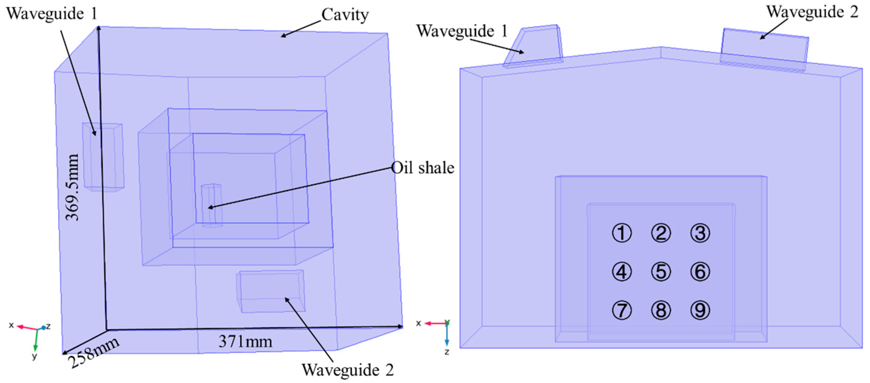
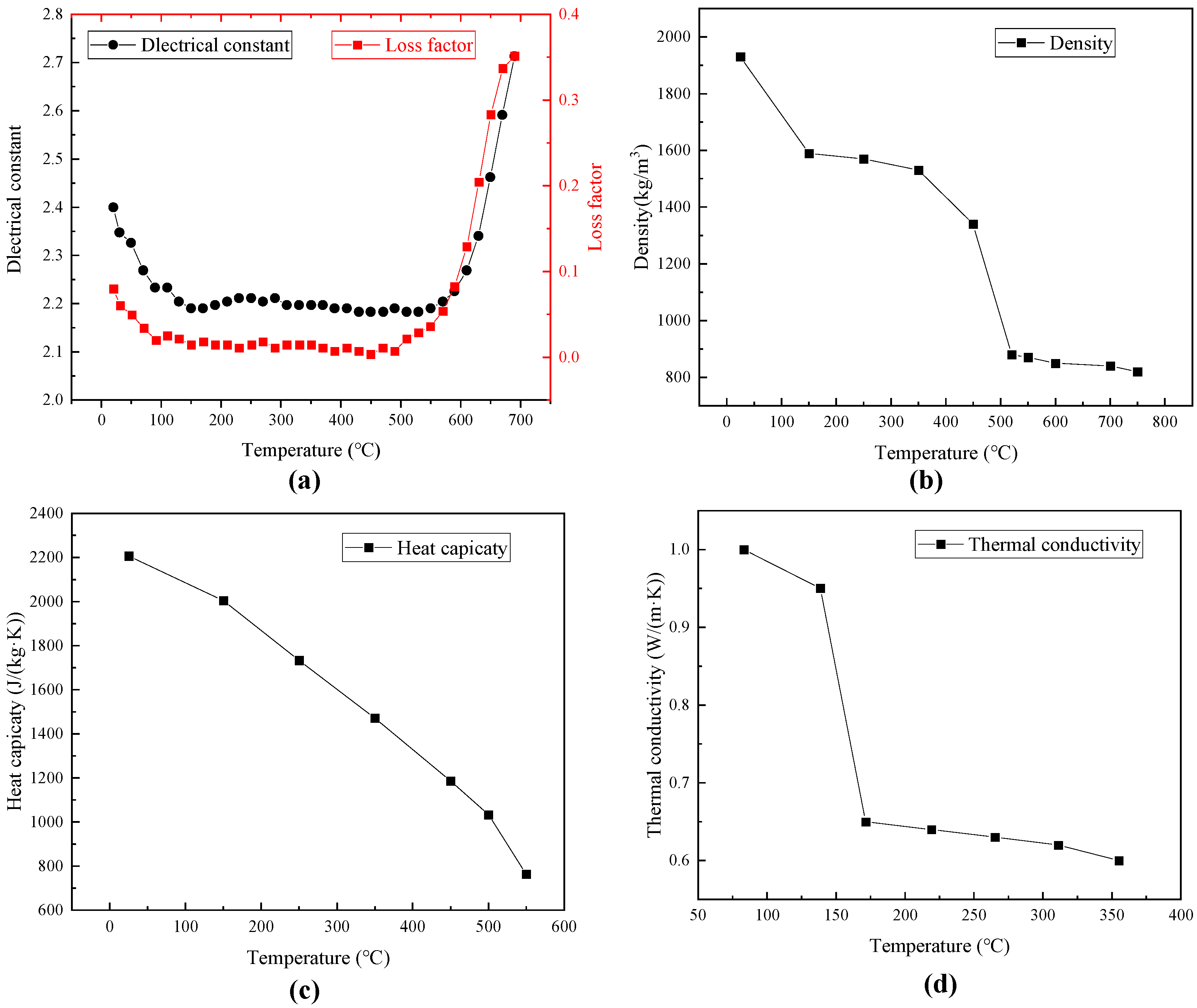
3.2. Geometry Model and Input Parameters

A cylindrical oil shale sample, with a diameter of 25 mm and length of 50 mm, was placed at the bottom of the oven, as shown in Figure 2. It is necessary to illustrate that sample positions 1–9 correspond to top central coordinates (220, −185, 165), (185, −185, 165), (150, −185, 165), (220, −185, 200), (185, −185, 200), (150, −185, 200), (220, −185, 235), (185, −185, 235), and (150, −185, 235), respectively.

The input parameters are listed in Table 2. Some temperature-dependent properties of oil shale, including the dielectric constant, loss factor, density, heat capacity, and thermal conductivity, were cited in this study as interpolation functions. Figure 3 shows the specific changes in the four parameters with increasing sample temperature. The thermodynamic properties of the mixture fluid were calculated based on the Peng–Robinson gas phase model established by the thermodynamic system in COMSOL Multiphysics.

Table 2. Parameters in this model.

Parameter	Symbol	Value	Source
Oil shale sample initial temperature	T0	20 °C	Given
Microwave frequency	f’	2.45 GHz	Given
Microwave power	P	1000 W	Given
Concentration of kerogen	c_ker	370 mol/m3	Ref. [33]
Molecular weight of kerogen	M_ker	647 g/mol	Ref. [34]
Molecular weight of heavy oil (C25H50)	M_ho	352 g/mol	Ref. [34]
Molecular weight of light oil (C9H20)	M_lo	128 g/mol	Ref. [34]
Molecular weight of non-hydrocarbon gas (CO2)	M_gas	44 g/mol	Ref. [34]
Molecular weight of methane (CH4)	M_ch	16 g/mol	Ref. [34]
Molecular weight of coke	M_coke	13 g/mol	Ref. [34]
Porosity of oil shale	ϕ	0.1	Measured
Permeability of oil shale	k	0.11 mD	Measured

Table 2. Parameters in this model.

Parameter	Symbol	Value	Source
Oil shale sample initial temperature	T0	20 °C	Given
Microwave frequency	f’	2.45 GHz	Given
Microwave power	P	1000 W	Given
Concentration of kerogen	c_ker	370 mol/m3	Ref. [33]
Molecular weight of kerogen	M_ker	647 g/mol	Ref. [34]
Molecular weight of heavy oil (C25H50)	M_ho	352 g/mol	Ref. [34]
Molecular weight of light oil (C9H20)	M_lo	128 g/mol	Ref. [34]
Molecular weight of non-hydrocarbon gas (CO2)	M_gas	44 g/mol	Ref. [34]
Molecular weight of methane (CH4)	M_ch	16 g/mol	Ref. [34]
Molecular weight of coke	M_coke	13 g/mol	Ref. [34]
Porosity of oil shale	ϕ	0.1	Measured
Permeability of oil shale	k	0.11 mD	Measured

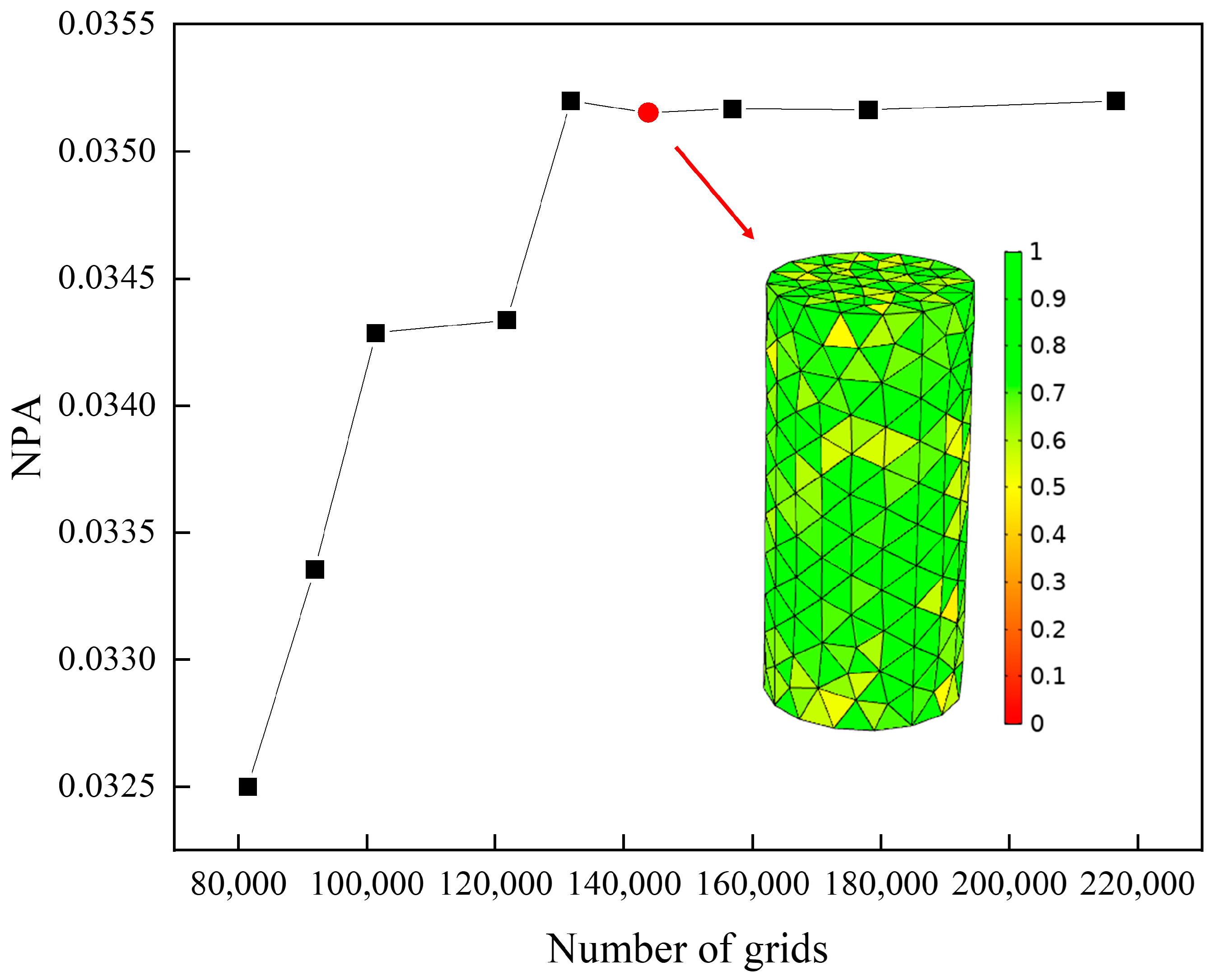
3.3. Grid-Independent Validation

To obtain accurate results, it is necessary to carry out grid-independent validation on account of the significant influence of mesh on finite element analysis results [38]. In this study, a variety of variable-size meshes were used to define the different domains; however, for all mesh sizes, the maximum element size was refined to below 1/6th of the microwave wavelength to carry out an accurate investigation of the pyrolysis characteristics. Tetrahedral elements were used for all the domains. The normalized absorbed power (NPA) is often used in mesh-independent studies [39,40]. When the value does not change with the increase in element number, the simulated results are independent from the mesh. The NPA of geometry under various element numbers is shown in Figure 4. When the grid number exceeded 143,820, the relative difference of NPA value did not exceed 0.04% of that of the finer grid. Therefore, a grid number of 143,820 was finally chosen during the whole numerical simulation.

The numerical models based on the finite element method (FEM) in this research were resolved by the COMSOL Multiphysics software [41]. The simulation was conducted on a workstation computer with an Intel Xeon CPU E5-2643 v4@ 3.40 GHz processor with 128 GB RAM memory and a 64-bit Windows 7 enterprise operating system.

3.4. Experimental Verifications

Three oil shale samples were collected from an open-pit mine in Maoming, Guadong province; their basic properties are presented in

Table 3. Analysis of three oil shale samples.

Item	Proximate Analysis (wt%)				Ultimate Analysis (wt%)					Porous Features
	Moisture	Volatiles	Ash	Fixed Carbon	H	O	N	S	C	Porosity	Permeability mD
S1	0.64	18.66	75.5	5.2	2.7	5.38	0.44	1.01	15.96	0.09	0.098
S2	0.98	17.32	75	6.7	2.88	5.98	0.66	1.11	17.32	0.08	0.087
S3	0.74	18.66	72.5	8.1	2.74	6.11	0.59	1.09	16.36	0.1	0.11

. For model verification, microwave experiments were conducted after oil shale dewatering. As shown in Figure 2, the structure of the microwave cavity was similar to the actual microwave apparatus, which helped to verify the correctness of the simulation model. The self-made microwave heating apparatus with a frequency of 2.45 GHz was used to irradiate the three oil shale samples. During irradiation, an armored thermocouple was used to test the surface temperature of the sample. The oil shale was heated at three power levels in the experiment and simulation under the same conditions, including 600 W, 800 W, and 1000 W. Figure 5 shows the temperature changes on the sample surface over time at the three different power levels. When the microwave power was 600 W, the experimental and numerical temperature curves were in good agreement. When the microwave power was increased, the experimental temperature was slightly lower than the numerical result. A fast heating rate easily leads to an excessive temperature region within the material, which causes intense heat and mass transfer from inside to outside. This result would decrease the temperature, especially for the surface temperature contacting the outside gas. Based on the above analysis, the numerical model established in our study is reliable and will be analyzed in the further discussion.

4. Results and Discussion

As a kind of electromagnetic wave, microwave frequency is typically 2.45 GHz or 0.915 GHz. Therefore, it is necessary to determine the appropriate frequency applied in the microwave apparatus. To be transported into the cavity, the microwave frequency must be larger than the cutoff frequency of the waveguide. For a rectangular waveguide, the propagation constant β is given by [42]:

$$\beta =\frac{2\pi }{c}\sqrt{f^2-f_c^2}$$

(20)

where f denotes the frequency of microwaves (Hz), f_c denotes the cutoff frequency (Hz), and c denotes the light velocity (m/s).

The cutoff frequency depends on the shape and size of the waveguide cross-section. The formula for the cutoff frequency of a rectangular cross-sectioned waveguide is given by [43]:

$$f_c=\frac{c}{2}\sqrt{{(\frac{m}{a})}^2+{(\frac{n}{b})}^2}$$

(21)

For the TE10 mode, the values of the mode numbers are m = 1 and n = 0, where a and b are the dimensions of the cross-section of the rectangular waveguides (cm). Therefore, the cutoff frequency in our model is defined as:

$$f_c=\frac{c}{2a}$$

(22)

Below this frequency, the waveguide attenuates or blocks the power. Based on Equation (22), the cutoff frequency in our model was 1.9 GHz. Therefore, other frequencies below 1.9 GHz, such as 0.915 GHz, could barely be transported into the cavity and could not be utilized in this study. Therefore, a frequency of 2.45 GHz was considered suitable for this simulation.

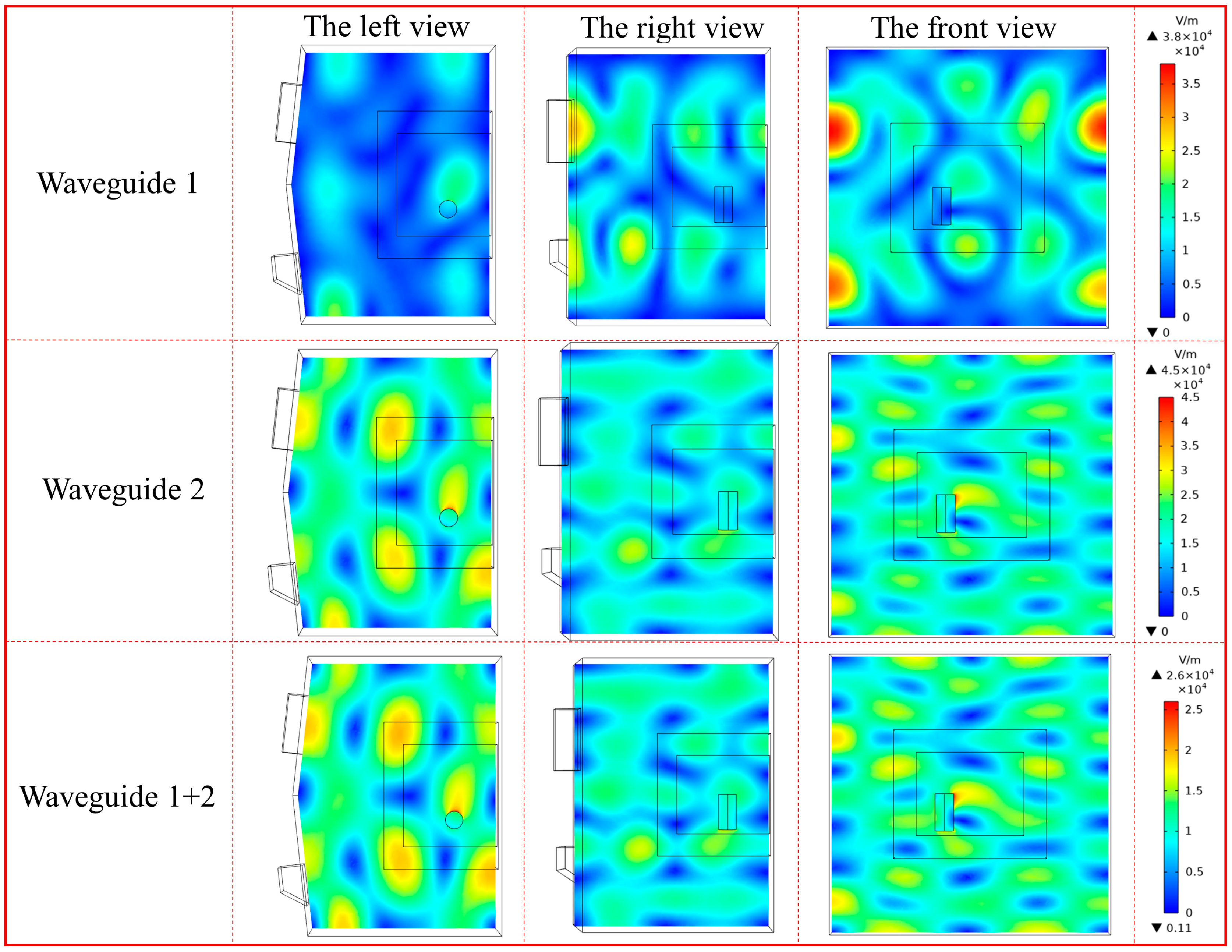
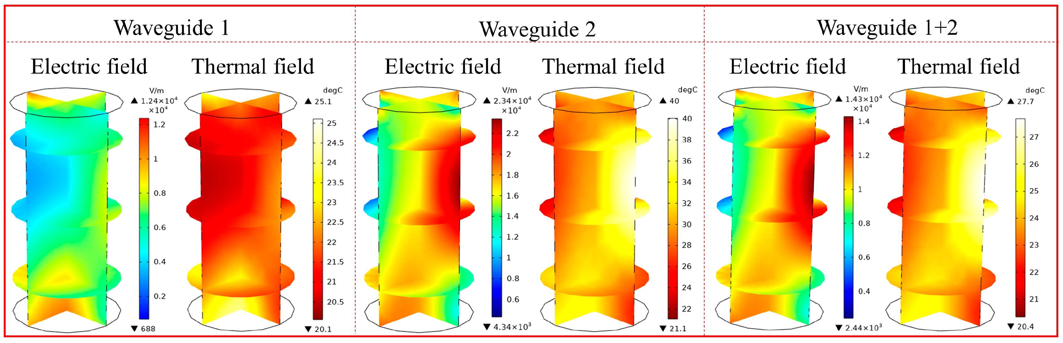
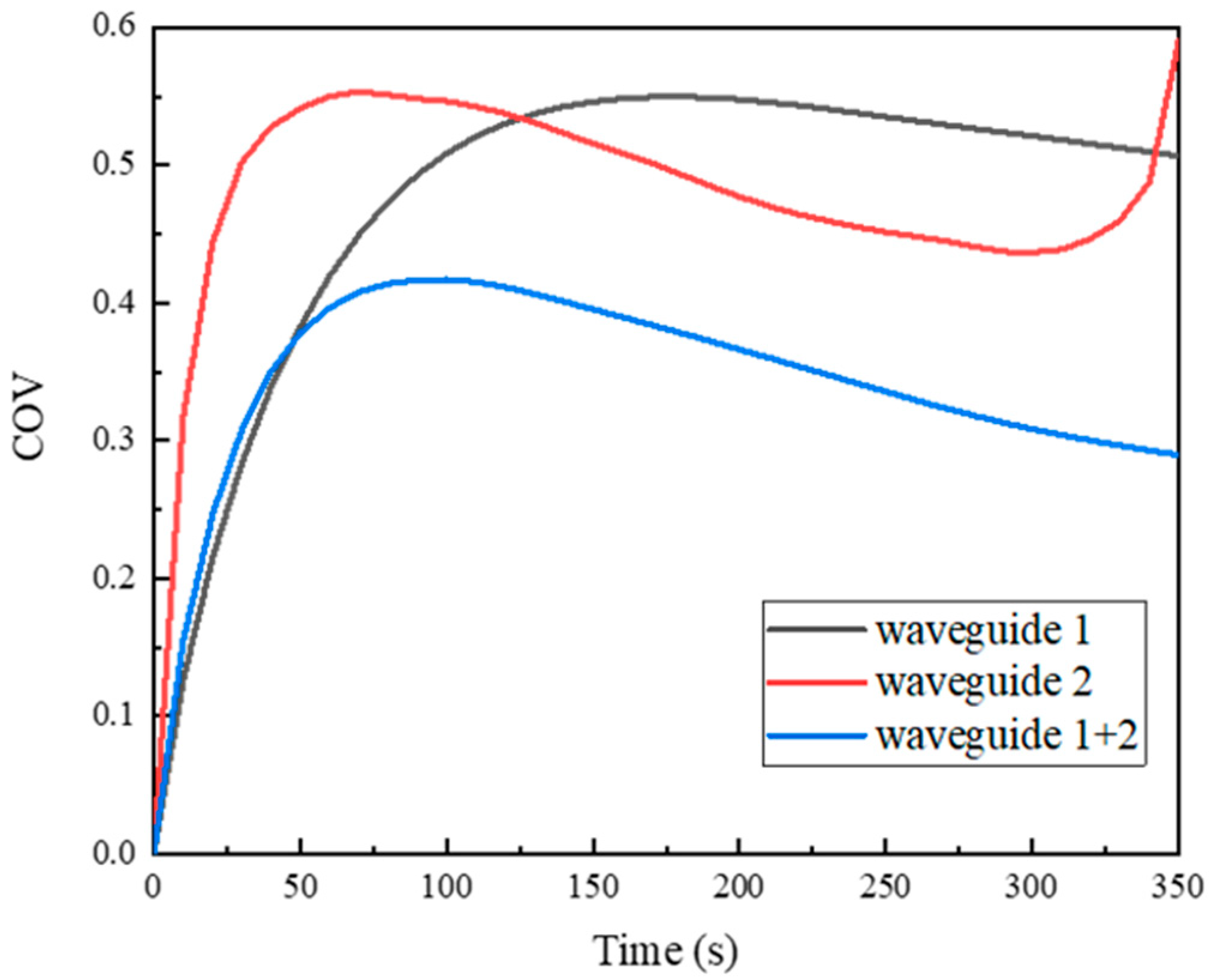
4.1. Effect of Microwave Waveguide

Although microwave irradiation has the advantage of a fast heating rate, there are also some defects associated with microwave heating, such as uneven temperature distribution. For oil shale pyrolysis, investigations have demonstrated that the secondary cracking of oil shale products occurs more easily at high temperatures [44]. To avoid excessive temperatures, changing the number and location of the waveguide may be a solution. The effect of the waveguide on the electric field of the oil shale is shown in Figure 6. In Figure 6, a three-view drawing including the left view, right view, and front view of the cavity is shown to reflect the electric distribution, which directly determines the temperature outcomes. For waveguide 1, the electric field distribution of the cavity was highly uneven, and its minimum and maximum electric field strengths were 0 V/m and 3.8 × 10⁴ V/m, respectively. For waveguide 2, the distribution was uneven, and its minimum and maximum electric field strengths were 0 V/m and 4.5 × 10⁴ V/m, respectively. For the double waveguide, the distribution seemed to be similar to that of waveguide 2; however, its minimum and maximum electric field strengths were 0.11 V/m and 2.6 × 10⁴ V/m, respectively, indicating that the electric field distribution under the double waveguide was more homogeneous than under the single waveguide. These phenomena indicate that the waveguide has a significant influence on the electric field of the microwave cavity, and the utilization of a double waveguide is helpful in obtaining a more uniform electric field.

Figure 7 shows the electric field and temperature distributions within oil shale. The electric field strength scope of waveguide 1, waveguide 2, and the double waveguide were 688–1.24 × 10⁴ V/m, 4.34 × 10³–2.34 × 10⁴ V/m, and 2.44 × 10³–1.43 × 10⁴ V/m, respectively. In addition, Figure 7 shows that the thermal field temperature distribution was similar to the electric field of the oil shale sample. To better evaluate the thermal uniformity within oil shale, the coefficient of variance was introduced, as shown in Equation (23).

$$\mathrm{COV}=\frac{1}{\overline{T}}\sqrt{\frac{1}{n}{\displaystyle \sum _{i=1}^n{\left(T_i-\overline{T}\right)}^2}}$$

(23)

Here, T_i and $\overline{T}$ denote the individual and average temperatures, respectively. The COV of the temperature indicates the deviation degree between the point temperature and the average value; a larger COV value represents a greater thermal heterogeneity. As shown in Figure 8, the COV curve of waveguide 1 first increased from 0 to 0.55 during 180 s and then gradually decreased to 0.507 at 350 s. The COV curve of waveguide 2 increased to 0.553 at 70 s, then decreased to 0.437 at 300 s, and finally increased sharply. When a double waveguide was used in microwave heating, its COV increased to 0.417 until 100 s and then gradually fell to 0.290. The peak of the COV under the double waveguide was less than the majority of the COV values under a single waveguide. Therefore, the operating condition of the double waveguide gained better temperature conformity than that of a single waveguide.

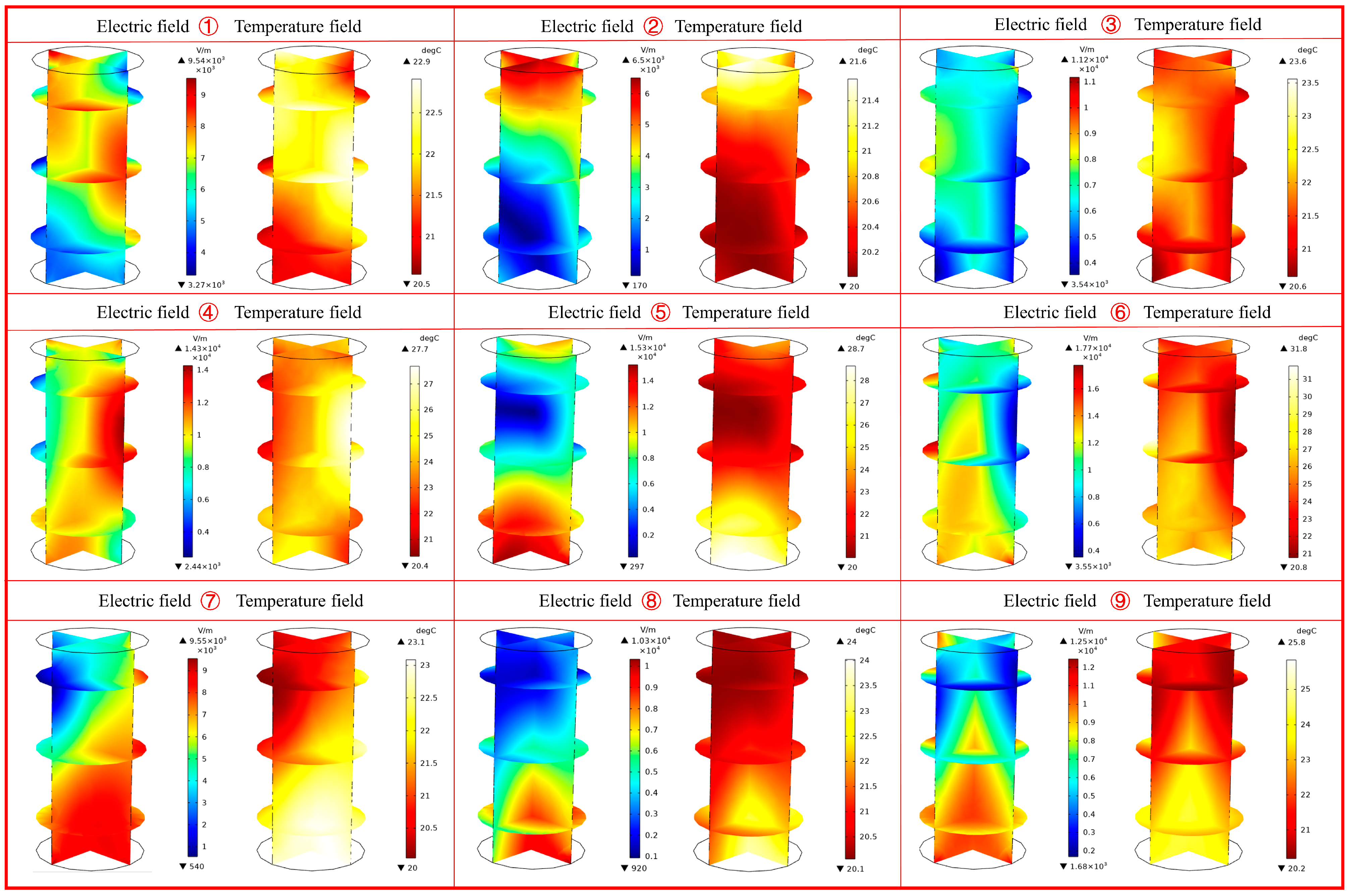
4.2. Effect of Sample Position

Double waveguides have been proven to be helpful in decreasing the temperature uniformity of samples during microwave heating; however, the sample position also influences its electric and temperature distribution. A schematic of the nine positions of the heated oil shale sample in the microwave apparatus is shown in Figure 2. It is necessary to illustrate that a double waveguide was used in this study, and the power was set to 1000 W.

As depicted in Figure 9, the electric field and temperature field of samples in different locations varied significantly, and the temperature distribution was also consistent with the electric field distribution. The oil shale at location 6 had the largest electric field strength and temperature compared to those in the other locations, whereas the oil shale at location 2 exhibited the minimum electric field strength and temperature. However, it is necessary to consider the effects of the heating efficiency and homogeneity simultaneously. On the one hand, in Figure 10a, the COV results demonstrate that locations 3, 4, 9, and 6 showed more uniform temperature distributions within the oil shale. On the other hand, Figure 10b shows the corresponding average temperature of oil shale during 800 s. It can be concluded that oil shale samples at locations 4 and 6 led to a higher temperature distribution. Therefore, to simultaneously achieve a high heating efficiency and low COV, location 4 is the best choice for oil shale pyrolysis.

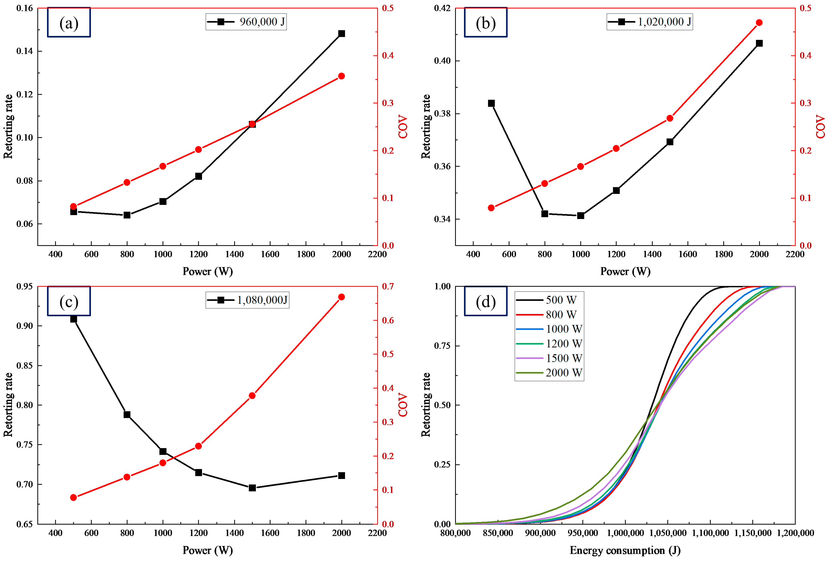
4.3. Effect of Microwave Power

Microwave power is an important parameter that influences the heating rate of oil shale. Moreover, the heating rate plays a significant role in oil shale pyrolysis on account of its considerable influence on the amount and composition of oil and gas products [45]. During oil shale pyrolysis, transformation efficiency and energy consumption should be considered simultaneously, and the microwave power can optimized based on the conditions of the double waveguide and location 4. Figure 11 shows the electric field and temperature distribution of the oil shale at different microwave powers after irradiation for 10 s. A higher microwave power led to a higher electric field intensity as well as maximum temperature, which is consistent with the results of many laboratory experiments.

To better understand the pyrolysis characteristics of oil shale under microwave heating, Figure 12a demonstrates that the average temperature of oil shale at different microwave powers had a similar upward trend. The higher the microwave power, the faster the heating rate. The temperature rise of oil shale could be characterized by “slow-fast”, and the turning point of the maximum temperature curve occurred at approximately 500 °C. This phenomenon results from the increase in the dielectric constant and loss factor of oil shale, as shown in Figure 3a. Moreover, as with the transformation of oil shale, there exists a heat source in exothermic chemical reactions. The pyrolysis rate is defined as the mass ratio of pyrolyzed kerogen to the original kerogen:

$$\mathrm{Pyrolysis}\mathrm{rate}=\frac{\mathrm{Mass}\mathrm{of}\mathrm{pyrolyzed}\mathrm{kerogen}}{\mathrm{Mass}\mathrm{of}\mathrm{original}\mathrm{kerogen}}$$

(24)

As shown in Figure 12b, once the pyrolysis was started, it could be completed in a short time, depending on the power value. In other words, a higher microwave power led to a shorter heating time. The energy consumption is defined as:

Energy consumption = Microwave power × Time

(25)

Table 4. Three energy consumption analysis schemes.

Energy Consumption of 960,000 J
Power (W)	500	800	1000	1200	1500	2000
Time (s)	1920	1200	960	800	640	480
Energy consumption of 1,020,000 J
Power (W)	500	800	1000	1200	1500	2000
Time (s)	2040	1275	1020	850	680	510
Energy consumption of 1,080,000 J
Power (W)	500	800	1000	1200	1500	2000
Time (s)	2160	1350	1080	900	720	540

shows three energy consumption analysis schemes to illustrate the pyrolysis effect with varying powers. In Figure 13d, all the curves of the oil shale pyrolysis rate with energy consumption at different power level resemble an “S” shape, while they have different slopes. For example, at a power of 500 W, the pyrolysis rate increased gradually compared with that at other powers before 1,000,000 J. However, after this, the pyrolysis rate increased rapidly and was the first one to finish the oil shale pyrolysis. When the power was 2000 W, the curve of the oil shale pyrolysis rate with energy consumption quickly increased, and the pyrolysis rate was higher than that at other powers before 1,025,000 J; however, the pyrolysis rate increased gradually afterwards. On the whole, a high power of 2000 W obtained a high pyrolysis rate at the initial stage and a low power of 500 W obtained a high pyrolysis rate at a later stage. To further analyze this regulation, Figure 13a–c show the pyrolysis rate changes and COV of oil shale temperature with power when the energy consumption was 960,000 J, 1,020,000 J, and 1,080,000 J, respectively. The COV of temperature always increased with microwave power, with the highest value corresponding to 2000 W and the lowest value corresponding to 500 W. The power of 2000 W yields the highest pyrolysis rate, whereas the lowest rate is obtained at 800 W, as shown in Figure 13a. As shown in Figure 13b, the power of 2000 W yields the highest pyrolysis rate, whereas the lowest rate occurs at 1000 W. The power of 500 W yielded the highest pyrolysis rate, whereas the lowest rate occurred at 1500 W, as shown in Figure 13c. Based on the above phenomena, it was concluded that a higher power leads to a higher COV, which implies that the spatial heterogeneity of the thermal fields increases considerably, owing to the higher microwave power. The lower power was associated with a lower COV, consuming less energy than that at a higher power during the pyrolysis process. The higher power was suitable for achieving a rapid temperature increase, whereas the lower power was suitable for achieving a high efficiency pyrolysis rate. The essence of this proposed method is variable microwave power, and it leverages the advantages of both high power and low power. The groups of 2000 W × 300 s and 500 W × 1085 s will be researched in the following study.

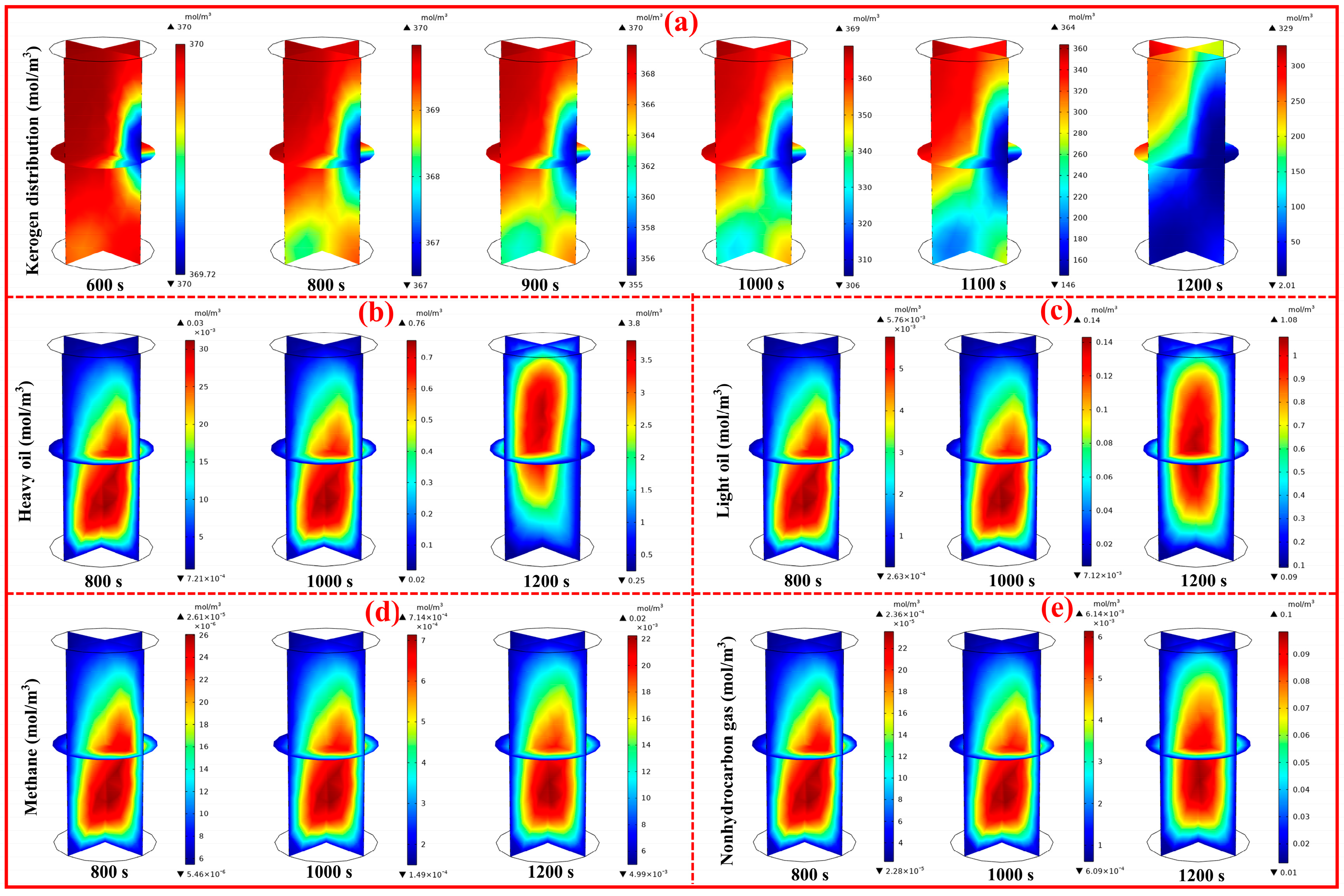
4.4. Analysis of Products Distribution

After optimizing the waveguide, sample position, and microwave power, the pyrolysis characteristics were analyzed based on the double waveguide, at location 4, with the variable power heating mode. Figure 14a shows the pyrolysis rate of the group of 2000 W × 300 s + 500 W × 1085 s. In Figure 14b, the profile slope of the average temperature at 500 W is smaller than that at 2000 W, and the final average temperature is 582.54 °C, which is less than the final average temperature at 2000 W. The COV of the temperature decreased after 300 s, indicating that the coupled power significantly improved the temperature distribution. The variable power heating mode was better than the single-power mode in terms of fast heating efficiency and uniform temperature distribution.

Based on the parameter optimization, Figure 15a shows the kerogen distribution within the oil shale sample over irradiation times. At 800 s, the minimum concentration of kerogen was 367 mol/m³ rather than the initial value of 370 mol/m³, revealing that kerogen started to decompose in the maximum temperature region. The thermal visualization showed that as the time increased, the blue area expanded in the entire area of the oil shale; this phenomenon is a strong direct indication of oil shale pyrolysis. As time went by, the kerogen under microwave heating transforms into various hydrocarbon chemicals, which can be categorized into four categories, including heavy oil, light oil, methane, and non-hydrocarbon gas, according to the reaction kinetics in Table 1. In Figure 15, the concentrations of the four products were different, but the distributions looked similar. To quantify the pyrolysis process, Figure 16 shows that a large amount of kerogen decomposition occurred near 1000 s, and the production of heavy oil and light oil decreased rapidly; when the heating time was close to 1290 s, a reduction in the concentration was observed, indicating the occurrence of secondary oil cracking. Additionally, the concentrations of methane and other non-hydrocarbon gases increased under microwave heating. Based on the production efficiency, methane has a low economic value, and non-hydrocarbon gas is considered as waste. Therefore, it is necessary to control the microwave parameters to optimize oil production. Specifically, the secondary reactions of oil products should be avoided as much as possible by controlling the temperature distribution of the oil shale.

Several kinds of heating methods for oil shale pyrosis are compared and analyzed in

Table 5. The comparison of different heating methods for oil shale pyrolysis.

Type of Heating	Benefits	Drawbacks	References
Supercritical carbon dioxide	Supercritical carbon dioxide can effectively extract organic matter from oil shale.	Prolonging the pyrolysis time and increasing the temperature can lead to the aggravation of secondary cracking.	[30]
Superheated water steam	Products have high mobility at high temperatures.	Oil shale with very low permeability hinders the entry of high-temperature steam.	[46,47]
In situ combustion	This technology conserves energy and decomposes the oil shale more thoroughly.	The pyrolysis and combustion process are extremely difficult to control.	[9,48]
Electric heating	Heating by the resistive loss technique is suited to achieving uniform heating. The corresponding research started early and this method is relatively fully studied.	The heating rate is slow and the energy consumption is very high.	[49,50,51]
Microwave heating	The temperature rise is fast and pyrolysis efficiency is high.	The uniformity of temperature distribution needs to be improved in the future.	This paper

, including supercritical carbon dioxide, superheated water steam, in situ combustion, electric heating, and microwave heating. Every approach has its benefits and drawbacks, and this paper provides guidance for enhancing the pyrolysis efficiency of oil shale under microwave heating.

5. Conclusions

A fully coupled three-dimensional electromagnetic-thermal-chemical-hydraulic model was successfully resolved based on the FEM to research the pyrolysis characteristics of oil shale irradiated by microwaves. This complex transformation process involves an electromagnetic field, heat transfer, mass transfer, and fluid flow. The temperature-dependent properties of oil shale, including dielectric constant, loss factor, heat capacity, and thermal conductivity, were considered. According to laboratory experiments, the simulated results were consistent with the experimental data, thus proving the reliability of the model.

Based on the analysis of the electric field and temperature distribution, the frequency, waveguide, and sample position were optimized as 2.45 GHz, double ports, and location 4, respectively. The utilization of a double waveguide is beneficial to obtain more a uniform electric field and heat transfer field. The electric field and temperature field of the sample in different locations varied significantly from each other, and there was an optimal location where the highest heating efficiency was obtained, which was on the left of the cavity center. A higher microwave power contributed to a faster temperature rise in the oil shale. The higher power was suitable for achieving a rapid temperature increase, while a lower power was suitable for achieving a high-efficiency pyrolysis rate. Therefore, a so-called variable power heating mode was proposed to decrease the heating time and improve the heat uniformity simultaneously during oil shale pyrolysis. The typical case of double ports, location 4, and variable power heating mode was selected to further investigate the mechanism of chemical product evaluation. The variable power heating mode showed better results than the single-power mode in terms of fast heating efficiency and uniform temperature distribution. Through the analysis of the transformation production distributions within oil shale, the results indicated that significantly high temperatures decreased the oil production, owing to secondary reactions. By optimizing the microwave heating parameters, the temperature distribution of the oil shale could be controlled, thereby enhancing the oil production. This study provides guidance for enhancing the pyrolysis efficiency of oil shale under microwave heating.

References

1. Zhang, Y.; Adam, M.; Hart, A.; Wood, J.; Rigby, S.P.; Robinson, J.P. Impact of Oil Composition on Microwave Heating Behavior of Heavy Oils. Energy Fuels 2018, 32, 1592–1599. [Google Scholar] [CrossRef]
2. Mead, I. International Energy Outlook 2017; US Energy Information Administration: Washington, DC, USA, 2017. Available online: https://csis-website-prod.s3.amazonaws.com/s3fs-public/event/170914_CSIS_release.pdf (accessed on 9 September 2021).
3. Xia, L.; Zhang, H.; Wang, B.; Yu, C. Numerical simulation and experimental validation of oil shale drying in pneumatic conveying dryer. Dry. Technol. 2018, 36, 617–629. [Google Scholar] [CrossRef]
4. Dong, F.; Feng, Z.; Yang, D.; Zhao, Y.; Elsworth, D. Permeability Evolution of Pyrolytically-Fractured Oil Shale under In Situ Conditions. Energies 2018, 11, 3033. [Google Scholar] [CrossRef] [Green Version]
5. Zou, C. Unconventional Petroleum Geology; Elsevier: Amsterdam, The Netherlands, 2017. [Google Scholar] [CrossRef]
6. Biglarbigi, K.; Crawford, P.; Carolus, M.; Dean, C. Rethinking World Oil-Shale Resource Estimates. In Proceedings of the SPE Annual Technical Conference and Exhibition, Florence, Italy, 20–22 September 2010. [Google Scholar] [CrossRef]
7. Song, X.; Zhang, C.; Shi, Y.; Li, G. Production performance of oil shale in-situ conversion with multilateral wells. Energy 2019, 189, 116145. [Google Scholar] [CrossRef]
8. Zheng, H.; Shi, W.; Ding, D.; Zhang, C. Numerical Simulation of In Situ Combustion of Oil Shale. Geofluids 2017, 2017, 3028974. [Google Scholar] [CrossRef] [Green Version]
9. Kang, Z.; Zhao, Y.; Yang, D. Review of oil shale in-situ conversion technology. Appl. Energy 2020, 269, 115121. [Google Scholar] [CrossRef]
10. Zhang, M.; Salazar-Tio, R.; Fager, A.; Crouse, B. A Multiscale Digital Rock Workflow for Shale Matrix Permeability Prediction. In Proceedings of the SPE/AAPG/SEG Unconventional Resources Technology Conference, Virtual, 20–22 July 2020. [Google Scholar] [CrossRef]
11. Taheri-Shakib, J.; Shekarifard, A.; Naderi, H. Characterization of the wax precipitation in Iranian crude oil based on Wax Appearance Temperature (WAT): Part 1. The influence of electromagnetic waves. J. Pet. Sci. Eng. 2018, 161, 530–540. [Google Scholar] [CrossRef]
12. Taheri-Shakib, J.; Shekarifard, A.; Naderi, H. The experimental study of effect of microwave heating time on the heavy oil properties: Prospects for heavy oil upgrading. J. Anal. Appl. Pyrolysis 2017, 128, 176–186. [Google Scholar] [CrossRef]
13. Taheri-Shakib, J.; Shekarifard, A.; Naderi, H. Analysis of the asphaltene properties of heavy crude oil under ultrasonic and microwave irradiation. J. Anal. Appl. Pyrolysis 2018, 129, 171–180. [Google Scholar] [CrossRef]
14. Hasanvand, M.Z.; Golparvar, A. A Critical Review of Improved Oil Recovery by Electromagnetic Heating. Pet. Sci. Technol. 2014, 32, 631–637. [Google Scholar] [CrossRef]
15. Zhu, J.; Yi, L.; Yang, Z.; Duan, M. Three-dimensional numerical simulation on the thermal response of oil shale subjected to microwave heating. Chem. Eng. J. 2021, 407, 127197. [Google Scholar] [CrossRef]
16. Chen, H.; Li, T.; Wang, Z.; Ye, R.; Li, Q. Effect of dielectric properties on heat transfer characteristics of rubber materials via microwave heating. Int. J. Therm. Sci. 2020, 148, 106162. [Google Scholar] [CrossRef]
17. Sun, Y.; Zhao, S.; Li, Q.; Liu, S.; Han, J. Thermoelectric coupling analysis of high-voltage breakdown industrial frequency pyrolysis in Fuyu oil shale. Int. J. Therm. Sci. 2018, 130, 19–27. [Google Scholar] [CrossRef]
18. Li, H.; Shi, S.; Lin, B.; Lu, J.; Ye, Q.; Lu, Y.; Wang, Z.; Hong, Y.; Zhu, X. Effects of microwave-assisted pyrolysis on the microstructure of bituminous coals. Energy 2019, 187, 115986. [Google Scholar] [CrossRef]
19. Qi, H.; Jiang, H.; You, Y.; Hu, J.; Wang, Y.; Wu, Z.; Qi, H. Mechanism of Magnetic Nanoparticle Enhanced Microwave Pyrolysis for Oily Sludge. Energies 2022, 15, 1254. [Google Scholar] [CrossRef]
20. Liu, J.; Wang, J.; Leung, C.; Gao, F. A Fully Coupled Numerical Model for Microwave Heating Enhanced Shale Gas Recovery. Energies 2018, 11, 1608. [Google Scholar] [CrossRef] [Green Version]
21. Amini, A.; Latifi, M.; Chaouki, J. Electrification of materials processing via microwave irradiation: A review of mechanism and applications. Appl. Therm. Eng. 2021, 193, 117003. [Google Scholar] [CrossRef]
22. Meng, Y.; Tang, L.; Yan, Y.; Oladejo, J.; Jiang, P.; Wu, T.; Pang, C. Effects of Microwave-enhanced Pretreatment on Oil Shale Milling Performance. Energy Procedia 2019, 158, 1712–1717. [Google Scholar] [CrossRef]
23. Al-Gharabli, S.I.; Azzam, M.O.J.; Al-Addous, M. Microwave-assisted solvent extraction of shale oil from Jordanian oil shale. Oil Shale 2015, 32, 240–251. [Google Scholar] [CrossRef] [Green Version]
24. Neto, A.; Thomas, S.; Bond, G.; Thibault-Starzyk, F.; Ribeiro, F.; Henriques, C. The Oil Shale Transformation in the Presence of an Acidic BEA Zeolite under Microwave Irradiation. Energy Fuels 2014, 28, 2365–2377. [Google Scholar] [CrossRef] [Green Version]
25. El Harfi, K.; Mokhlisse, A.; Chanâa, M.B.; Outzourhit, A. Pyrolysis of the Moroccan (Tarfaya) oil shales under microwave irradiation. Fuel 2000, 79, 733–742. [Google Scholar] [CrossRef]
26. Scaar, H.; Franke, G.; Weigler, F.; Delele, M.; Tsotsas, E.; Mellmann, J. Experimental and numerical study of the airflow distribution in mixed-flow grain dryers. Dry. Technol. 2016, 34, 595–607. [Google Scholar] [CrossRef]
27. Jamaleddine, T.J.; Ray, M.B. Application of Computational Fluid Dynamics for Simulation of Drying Processes: A Review. Dry. Technol. 2010, 28, 120–154. [Google Scholar] [CrossRef]
28. Skuratovsky, I.; Levy, A.; Borde, I. Two-Fluid, Two-Dimensional Model for Pneumatic Drying. Dry. Technol. 2003, 21, 1645–1668. [Google Scholar] [CrossRef]
29. Mezhericher, M.; Levy, A.; Borde, I. Three-dimensional modelling of pneumatic drying process. Powder Technol. 2010, 203, 371–383. [Google Scholar] [CrossRef]
30. Zhao, S.; Lü, X.; Li, Q.; Sun, Y. Thermal-fluid coupling analysis of oil shale pyrolysis and displacement by heat-carrying supercritical carbon dioxide. Chem. Eng. J. 2020, 394, 125037. [Google Scholar] [CrossRef]
31. Wang, Q.; Pan, S.; Bai, J.; Chi, M.; Cui, D.; Wang, Z.; Liu, Q.; Xu, F. Experimental and dynamics simulation studies of the molecular modeling and reactivity of the Yaojie oil shale kerogen. Fuel 2018, 230, 319–330. [Google Scholar] [CrossRef]
32. Zhu, J.; Yi, L.; Yang, Z.; Li, X. Numerical simulation on the in situ upgrading of oil shale reservoir under microwave heating. Fuel 2021, 287, 119553. [Google Scholar] [CrossRef]
33. Youtsos, M.S.K.; Mastorakos, E.; Cant, R.S. Numerical simulation of thermal and reaction fronts for oil shale upgrading. Chem. Eng. Sci. 2013, 94, 200–213. [Google Scholar] [CrossRef]
34. Lee, K.J.; Moridis, G.J.; Ehlig-Economides, C.A. Numerical simulation of diverse thermal in situ upgrading processes for the hydrocarbon production from kerogen in oil shale reservoirs. Energy Explor. Exploit. 2017, 35, 315–337. [Google Scholar] [CrossRef] [Green Version]
35. Al-Harahsheh, M.; Kingman, S.; Saeid, A.; Robinson, J.; Dimitrakis, G.; Alnawafleh, H. Dielectric properties of Jordanian oil shales. Fuel Process. Technol. 2009, 90, 1259–1264. [Google Scholar] [CrossRef]
36. Wang, L. Experiment and Simulation on Temperature Field during Oil Shale Pyrolysis by Electric-Heating. Master’s Thesis, Jilin University, Changchun, China, 2014. Available online: https://kns.cnki.net/kcms/detail/detail.aspx?FileName=1014268510.nh&DbName=CMFD2014 (accessed on 17 January 2022).
37. Nottenburg, R.; Rajeshwar, K.; Rosenvold, R.; DuBow, J. Measurement of thermal conductivity of Green River oil shales by a thermal comparator technique. Fuel 1978, 57, 789–795. [Google Scholar] [CrossRef]
38. Tamang, S.; Aravindan, S. 3D numerical modelling of microwave heating of SiC susceptor. Appl. Therm. Eng. 2019, 162, 114250. [Google Scholar] [CrossRef]
39. Zhou, J.; Yang, X.; Ye, J.; Zhu, H.; Yuan, J.; Li, X.; Huang, K. Arbitrary Lagrangian-Eulerian method for computation of rotating target during microwave heating. Int. J. Heat Mass Transf. 2019, 134, 271–285. [Google Scholar] [CrossRef]
40. He, J.; Yang, Y.; Zhu, H.; Li, K.; Yao, W.; Huang, K. Microwave heating based on two rotary waveguides to improve efficiency and uniformity by gradient descent method. Appl. Therm. Eng. 2020, 178, 115594. [Google Scholar] [CrossRef]
41. Huang, X.; Rudolph, D.L. Coupled model for water, vapour, heat, stress and strain fields in variably saturated freezing soils. Adv. Water Resour. 2021, 154, 103945. [Google Scholar] [CrossRef]
42. Abo Seida, O.M. Propagation of electromagnetic waves in a rectangular tunnel. Appl. Math. Comput. 2003, 136, 405–413. [Google Scholar] [CrossRef]
43. Huang, J.; Xu, G.; Hu, G.; Kizil, M.; Chen, Z. A coupled electromagnetic irradiation, heat and mass transfer model for microwave heating and its numerical simulation on coal. Fuel Process. Technol. 2018, 177, 237–245. [Google Scholar] [CrossRef]
44. Shekarifard, A.; Taheri-Shakib, J. Technical and scientific review on oil shale upgrading. Int. J. Petrochem. Sci. Eng. 2016, 1, 78–83. [Google Scholar] [CrossRef]
45. Taheri-Shakib, J.; Kantzas, A. A comprehensive review of microwave application on the oil shale: Prospects for shale oil production. Fuel 2021, 305, 121519. [Google Scholar] [CrossRef]
46. Wang, L.; Yang, D.; Kang, Z. Evolution of permeability and mesostructure of oil shale exposed to high-temperature water vapor. Fuel 2021, 290, 119786. [Google Scholar] [CrossRef]
47. Wang, G.; Liu, S.; Yang, D.; Fu, M. Numerical study on the in-situ pyrolysis process of steeply dipping oil shale deposits by injecting superheated water steam: A case study on Jimsar oil shale in Xinjiang, China. Energy 2022, 239, 122182. [Google Scholar] [CrossRef]
48. Sun, Y.; Bai, F.; Liu, B.; Liu, Y.; Guo, M.; Guo, W.; Wang, Q.; Lü, X.; Yang, F.; Yang, Y. Characterization of the oil shale products derived via topochemical reaction method. Fuel 2014, 115, 338–346. [Google Scholar] [CrossRef]
49. Martemyanov, S.; Bukharkin, A.; Koryashov, I.; Ivanov, A. Analysis of applicability of oil shale for in situ conversion. AIP Conf. Proc. 2016, 1772, 020001. [Google Scholar] [CrossRef] [Green Version]
50. Hao, Y.; Xiaoqiao, G.; Fansheng, X.; Jialiang, Z.; Yanju, L. Temperature distribution simulation and optimization design of electric heater for in-situ oil shale heating. Oil Shale 2014, 31, 105–120. [Google Scholar] [CrossRef] [Green Version]
51. Ryan, R.C.; Fowler, T.D.; Beer, G.L.; Nair, V. Shell’s In Situ Conversion Process—From Laboratory to Field Pilots. In Oil Shale: A Solution to the Liquid Fuel Dilemma; American Chemical Society: Washington, DC, USA, 2010; Volume 1032, pp. 161–183. [Google Scholar] [CrossRef]
Figure 1. The coupling relationship among the governing equations for the microwave pyrolysis of oil shale.
Energies 15 03256 g001
Figure 2. Geometry model of microwave oven and its nine sample positions in the simulation.
Energies 15 03256 g002
Figure 3. Oil shale properties dependent on temperature: (a) dielectric constant and loss factor [35], (b) density [36], (c) heat capacity [30], and (d) thermal conductivity [37].
Energies 15 03256 g003
Figure 4. Grid-independent validation of the simulation.
Energies 15 03256 g004
Figure 5. Sample surface temperature of simulation and experimental oil shale under different power levels.
Energies 15 03256 g005
Figure 6. Three-view drawing of the electric field distribution excited by different microwave sources.
Energies 15 03256 g006
Figure 7. Electric field and temperature distribution within the oil shale sample in the presence of different numbers of waveguides at 10 s.
Energies 15 03256 g007
Figure 8. Relationship between the coefficient of variance of the temperature and microwave heating time at different waveguide excitations.
Energies 15 03256 g008
Figure 9. Electric field and temperature field strength and distribution of the nine positions of the heated sample domain after heating for 10 s.
Energies 15 03256 g009
Figure 10. Volumetric average temperature and its COV of oil shale sample at locations 1–9 during 800 s: (a) COV and (b) average temperature.
Energies 15 03256 g010
Figure 11. Electric field and temperature field of sample at different microwave powers after 10 s.
Energies 15 03256 g011
Figure 12. Average temperature and pyrolysis rate of oil shale with time at different microwave powers during 2500 s: (a) average temperature and (b) pyrolysis rate.
Energies 15 03256 g012
Figure 13. Relationship of microwave power, pyrolysis rate, and COV of temperature of oil shale pyrolysis under varying energy consumptions: (a) energy consumption of 960,000 J, (b) energy consumption of 1,020,000 J, (c) energy consumption of 1,080,000 J, and (d) relationship between pyrolysis rate and energy consumption.
Energies 15 03256 g013
Figure 14. (a) Pyrolysis rate of oil shale with energy consumption. (b) Relationship of oil shale average temperature and heating time on the left Y-axis, and relationship of oil shale COV of temperature and heating time on the right Y-axis.
Energies 15 03256 g014
Figure 15. Kerogen distribution in oil shale for the group of 2000 W × 300 s and 500 W × 1085 s at six moments of 600 s, 800 s, 900 s, 1000 s, 1100 s, and 1200 s; products distribution after kerogen decomposition at 800 s, 1000 s, and 1200 s: (a) kerogen, (b) heavy oil, (c) light oil, (d) methane, and (e) non-hydrocarbon gas.
Energies 15 03256 g015
Figure 16. Relationship between time and average product concentration in heating oven.
Energies 15 03256 g016