Rational Application of Electric Power Production Optimization through Metaheuristics Algorithm

Abstract

The aim of this manuscript is to introduce solutions to optimize economic dispatch of loads and combined emissions (CEED) in thermal generators. We use metaheuristics, such as particle swarm optimization (PSO), ant lion optimization (ALO), dragonfly algorithm (DA), and differential evolution (DE), which are normally used for comparative simulations, and evaluation of CEED optimization, generated in MATLAB. For this study, we used a hybrid model composed of six (06) thermal units and thirteen (13) photovoltaic solar plants (PSP), considering emissions of contaminants into the air and the reduction in the total cost of combustibles. The implementation of a new method that identifies and turns off the least efficient thermal generators allows metaheuristic techniques to determine the value of the optimal power of the other generators, thereby reducing the level of pollutants in the atmosphere. The results are presented in comparative charts of the methods, where the power, emissions, and costs of the thermal plants are analyzed. Finally, the comparative results of the methods were analyzed to characterize the efficiency of the proposed algorithm.

1. Introduction

The energy crises that occur worldwide can be managed through the connection of sustainable and renewable energy systems, which are needed as we attempt to reduce the use of fossil fuels as populations increase. Interconnected grids can be divided into a power system structure based on the joint operations to generate and transmit power to the load demand as operational and technical controls [1,2,3].

The standard economic load dispatch (ELD) solution seeks to assign the total power demand among all generators used to achieve the minimum fuel cost [4]. Deterministic methods applied in the ELD solution are difficult to apply because of the non-continuous, non-convex, and nonlinear nature of the problem [5,6]. However, new rules have forced Thermoelectric Power Plant (TPP) to reduce the amount of polluting emissions into the atmosphere, expanding the ELD issue to the economic combined emissions dispatch (CEED) created to minimize fuel costs and pollutant emissions such as NO_x, SO_x, and CO_x elements from the TPP. Although the ELD and CEED problems are nonlinear optimization problems, many heuristic methods have been implemented to solve them, CEED is a multi-objective optimization [7,8]. The concept of the price penalty factor was proposed by some researchers to transform the CEED multi-objective issue into a single-objective issue by unifying the emission cost equations with the fuel cost equations [9,10].

Many techniques have been proposed to solve the ELD problem in power systems [11,12,13], and a nonconvex ELD difficulty has been addressed by several hybrid optimization techniques. According to [14], a technique based on particle swarm optimization with constriction factor (CFPSO) was proposed for ELD with valve point effects, which proved to have fast convergence. In [15], a CEED solution was recommended using the Artificial Bee Colony (ABC) algorithm. In [16,17] the distribution network reconfiguration was optimized using the dragonfly algorithm (DA). In [18], the energy balances in the ELD were solved by constraining its power generation capacity limits using Ant Lion Optimization (ALO). In [14], multi-objective particle swarm optimization (MOPSO) was performed using a diversity preservation mechanism to obtain a wide range of Pareto optimal solutions. Several hybrid techniques that combine two or more evolutionary optimization metaheuristics can improve the optimization results used in ELD [19,20].

Different mathematical methods and genetic algorithms (GAs) were applied to solve the ELD [21], including in studies [22] which applied DE studies and [23] used the multi-objective DE technique to solve EELD. In [24,25], it was the multi-objective techniques of NSGA II and Evolutionary Programming used to solve environmental and economic dispatches. In [7,26], the economic dispatch of a power system included wind and solar thermal energy. In [27], author considered regulatory, tariff, and economic mechanisms in distributed generation, for photovoltaic systems connected to the grid. In [28], the no free lunch (NFL) theorems for optimization were proposed. The NFL theorem states that a single algorithm does not work equally well in all optimization problems.

The purpose of this manuscript consists of the optimization of the production of electricity in grid safety standards, in addition to proving the effectiveness of the Differential Evolution (DE) metaheuristic allied to the shutdown of less efficient engines, obtaining significant reductions in generation costs and emissions of polluting gases in the atmosphere, maintaining the balance of the electrical grid after the insertion of photovoltaic solar energy. The study compares four (4) metaheuristic techniques to find the best solution to the CEED problem.

2. Problem Formulation

To streamline the multicriteria issue of CEED, two objective functions must be considered: one for oil consumption f₁(P_i) and one for environmental cost f₂(P_i) [29]. The objective function coefficients are achieved by adjusting the techniques of the curves based on the generator performance test [30,31].

2.1. Mathematical Model of Generation by Solar Power Plant (g₁)

The model of solar power plant generation (SPP) is described in Equation (1) [8,32,33,34]:

$$g_1\left(Pg{s}_j\right)=P_{rated} \left(1+\left(T_{ref}-T_{amb}\right)\ast alpha\right)\ast \frac{S_i}{1000}$$

(1)

where:

• g₁ = solar power plant
• Pgs_j = generated power by the solar plant
• P_rated = rated power;
• T_ref = reference temperature;
• T_amb = room temperature;
• alpha = temperature coefficient; and
• S_i = incident solar radiation.

With the contribution of the SPP stemming system, the added solar energy is described in (2) [8,32,33,34]:

$$Ss={{\displaystyle \sum }}_{j=1}^m{F}_1\left(Pg{s}_j\right)\times U{s}_j$$

(2)

where $Pg{s}_j$ is the energy available at the jth SPP and $U{s}_j$ indicates the status of the jth SPP, which is 1 (ON) or 0 (OFF). The cost of the SPP is given by (3) [8]:

$$Sc={{\displaystyle \sum }}_{j=1}^{m}PUCos{t}_j\times F_1\left(Pg{s}_j\right)\times U{s}_j$$

(3)

where $PUCos{t}_j$ is the unit cost of jth SPP.

2.2. Mathematical Model of Cost of Thermal Plants (f₁)

The principal ELD characteristic is to ascertain the optimum energy demand between the generating units of the station, minimize the total operational cost, and satisfy one cluster of restrictions of equality and inequality, which is one of the principal tasks of energy system optimization. Due to environmental responsibility, ELD was devoted to a multi-criterion optimization issue of CEED, aiming to reduce the emission of pollutant gases in the atmosphere [35].

The equation for the fuel consumption of every unit is represented by the quadratic function in Equation (4), considering the generator output power P_i, given as $/h, as in [4]:

$$f_i\left(P_i\right)=a_i+b_i{P}_i+c_i{P}_i^2$$

(4)

where, $a_i$ $b_i$ and $c_i$ represent the fuel consumption coefficients of each generating unit.

The problem of minimizing the total cost of a TPP is represented by Equation (5):

$$Min f_1\left(P_i\right)={{\displaystyle \sum }}_{i=1}^N{f}_i\left(P_i\right)$$

(5)

where N is the total number of generating units of the TPP and $P_i$ is the output power of each generating unit.

2.3. Mathematical Model of Emissions of Thermal Plants (f₂)

The function of the total thermal station emissions formulated in Equation (6) relates the emission to the power generated by every generator unit. This function represents the emission of SO₂ and NO_x in kg/h, which can be expressed as [4,9,29,36]:

$$h_i\left(P_i\right)={\alpha }_i+{\beta }_i{P}_i+{\gamma }_i{P}_i^2$$

(6)

where ${\alpha }_i$ ${\beta }_i$ and ${\gamma }_i$ represent the emission coefficients of all generating units.

Equation (7) represents the total minimizations of the TPP problem.

$$Min f_2\left(P_i\right)={{\displaystyle \sum }}_{i=1}^N{h}_i\left(P_i\right)$$

(7)

where N is the total number of generators in the TPP and $P_i$ is the energy output of each generator.

2.4. Economical Load Dispatch Constrains

2.4.1. Equal Power Constraints

The Equation (8) is expressed as a parity constraint on the nominal power, given the lower and upper bounds of each unit, following [37,38]:

$${{\displaystyle \sum }}_{i=1}^n{P}_i-P^D-P^L=0$$

(8)

where $P_i$ is the nominal power, $P^D$ is the power demand, $P^L$ is the transmission loss.

Therefore, the total generation should be similar to the power demand, plus the actual loss in the transmission lines. According to Equation (9):

$${{\displaystyle \sum }}_{i=1}^n{P}_i=P^D+P^L$$

(9)

The restriction on the total power generated in Equation (8) considers the total power generated by the SPP, that is, Equation (10) [8].

$$P^D+P^L-{{\displaystyle \sum }}_{i=1}^n{P}_i-{{\displaystyle \sum }}_{j=1}^{m}Pg{s}_j\times U{s}_j=0$$

(10)

The P^L dimensioning is equal to the sum of losses versus power, which have the same active and reactive power constraints at each bar according to Equation (11) [25]:

$$P^L={{\displaystyle \sum }}_{i=1}^n{B}_i P_i^2$$

(11)

Transmittance losses are defined as an output generator function arising from the Kron loss coefficients of Kron’s loss formula, Equation (12) [38,39]:

$$P^L={{\displaystyle \sum }}_{i=1}^n{{\displaystyle \sum }}_{j=1}^m{P}_j B_{ij} P_j+{{\displaystyle \sum }}_{i=1}^n{B}_{oi} P_j+B_{oo}$$

(12)

where B_ij, B_oi, and B_oo are the coefficients of the system transmission loss, and n is the generator number. The B coefficients can be accurately identified when the actual operating conditions are close to the base case [38,39].

2.4.2. Generation Constraint

Equation (13) expresses the power of each generating unit by the upper and lower limits, according to [31,40,41]:

$$P_{min.i }\le P_i \le P_{max.i}$$

(13)

where $P_i$ is the output power of each generating unit and $P_{min.i }$ and $P_{max.i}$ are the minimum and maximum power of the generator.

Another constraint that has to be met in a mixed system with photovoltaics is to maximize the utilization to 80% of SPP capacity installed, owing to the generator instability, presented in Equation (14) [8]:

$${{\displaystyle \sum }}_{j=1}^{m}Pg{s}_j\times U{s}_j\le 0.8\times SPP$$

(14)

2.5. Optimization Problem

For this issue, the energy generation is calculated by analyzing the SPP capacity installed; maximum value is being utilized to 80% of the total generation, and then the SPP energy generation is calculated, applying the function g₁ (Pgs_j) described in (1). The remaining pendent demand is solved by minimizing the multi-criteria problem in Equation (15):

$$Min=\left[f_1\left(Pi\right),f_2\left(Pi\right)\right]$$

(15)

where f₁(P_i) and f₂(P_i) are the objective functions of the costs and emissions, respectively, to be optimized.

2.6. Formulation of the Incremental Cost

The incremental cost of oil ($/MWh) is given by Equation (16) [42]:

$$I{C}_i=\left(2·a_i·P_{gi}+b_i\right)$$

(16)

where:

• $I{C}_i$ = incremental fuel cost;
• $a_i$ = actual incremental cost curve;
• $b_i$ = is an approximate (linear) incremental cost curve;
• $P_{gi}$ = total power generation.

3. Optimization Technique

Despite using different techniques and methods to solve the CEED, new and innovative algorithms are still being proposed for the solution. The main intrinsic motivation for this is the theorem No Free Lunch (NFL) [43]. The NFL theorem states that a single algorithm does not work as accurately for all optimization problems. Therefore, it is justified to search for new, more suitable algorithms and to refine existing algorithms.

To experiment with this theory and seek new results, we used the DA, DE, and ALO techniques to compare the results of the three techniques to determine the one that can obtain better solutions to the CEED problem.

▪

A new swarm intelligence optimization technique called the DA was proposed by [44]. This technique considers the proposal of binary and multi-objective versions. Dragonflies are small predators that hunt almost every small insect in nature. An interesting fact about dragonflies is their unique and rare swarming behavior. Dragonflies group together for two purposes: the first being hunting (static) and the second being migration (dynamic swarm). The hunting is in small groups. Dynamic swarms form large groups and travel long distances [44,45,46,47].

▪

To point out three primitive principles of swarm behavior [44,47]:

○

Separation is about preventing static collisions of individuals with other individuals in the neighborhood.

○

The alignment indicates the similar speed of the individuals with that of other individuals in the neighborhood.

○

Cohesion refers to the predisposition of individuals to move toward the center of mass in the neighborhood.

For any swarm its survival is necessary, so all individuals must be attracted to its food sources to avoid confrontation with external enemies.

Each of these behaviors is mathematically modeled as follows:

The separation is calculated as follows [44,47]:

$$S_i=-{{\displaystyle \sum }}_{j=1}^{N}X-X_j$$

(17)

where X is the current individual, X_j is the position of the jth neighboring individual, and N is the number of neighboring individuals.

The positioning is calculated by Equation (18):

$$A_i=\frac{{{\displaystyle \sum }}_{j=1}^N{V}_j}{N}$$

(18)

where V_j denotes the velocity of the jth neighboring individual.

Cohesion is calculated as follows:

$$C_i=\frac{{{\displaystyle \sum }}_{j=1}^N{X}_j}{N}-X$$

(19)

where X is the position of the current individual, N is the number of neighborhoods, and X_j is the position of the jth neighbor individual.

Attraction to a food source is calculated as follows:

$$F_i=X^{+}-X$$

(20)

where X is the location of the current individual and X⁺ is the position of the food source.

The Equation (21) shows the division to the outside of an enemy individual:

$$E_i=X^{-}+X$$

(21)

where X is the position of the current individual and $X^{-}$ shows the position of the enemy.

The dragonfly assumes a behavior based on five patterns. To update the positions of the artificial dragonflies at a search location and simulate their displacements, two vectors were considered: pitch (∆X) and position (X). The pitch vector is similar to the velocity vector in PSO, and the DA algorithm is developed based on the structure of the PSO algorithm. The pitch vector shows the direction of displacements of dragonflies; however, the introduced method can be extended to higher dimensions [44,46,47].

▪

For DE, [48,49] proposed a new encoded evolution algorithm using a fluctuating point for global optimization and was nominated as DE algorithm. DE has four main stages: initialization, mutation, crossover, and selection. Many optimization guidelines should also be adjusted. These guidelines are bonded under the control guidelines of the common name. There are only three guidelines for the real control of the algorithm: the differential constant F (or mutation), crossover constant Cr, and population length Np. The remaining guideline dimensions of issue D measure optimization task difficulty, and generation maximum number (or iteration) Gen. This can be suited as an interruption condition, and low and high limit restrictions are variables that range a viable area [41,48,50].

The ith vector of current population G with size D can be defined by:

$${\overrightarrow{X}}_{i,G}=\left[X_{1,i,G},X_{2,i,G},X_{3,i,G};\dots ;X_{D,i,G}\right], \{\begin{array}{c}i=0,1,\dots ,Np-1\\ j=1,\dots ,D \end{array}$$

(22)

Initialization: The initialization of the DE uses Np D-dimensional real-valued parameter vectors to perform random generation of candidate solutions.

$$X_{j,i,0}=X_{j,min}+ran{d}_{ij}\left[0,1\right]\left(X_{j,max}-X_{j,min}\right)$$

(23)

where $ran{d}_{ij}\left[0,1\right]$ is a random number, $0\le ran{d}_{ij}\left[0,1\right]\le 1$ which is multiplied by the interval length, $\left(X_{j,max}-X_{j,min}\right)$ ensures a distributed sampling of the parameter’s domain interval $\left[X_{j,min},X_{j,max}\right]$.

Different approaches with random uniformity are the most common, so they are used to generate the initial population [50,51].

Mutation: Mutation: Differential mutation adds a random-scale vector subtraction to a third vector. The vectors of the variable ${\overrightarrow{V}}_{i,G}$, also called donors, are obtained by this operation [50,51]:

$${\overrightarrow{V}}_{i,G}={\overrightarrow{X}}_{r_1^i,G}+F\left({\overrightarrow{X}}_{r_2^i,G}-{\overrightarrow{X}}_{r_3^i,G}\right)$$

(24)

where F > 0 is a real number that controls the growth rate of a population. Vectors ${\overrightarrow{X}}_{r_1^i,G}, {\overrightarrow{X}}_{r_2^i,G} \mathrm{and} {\overrightarrow{X}}_{r_3^i,G}$ from the current population the samples are randomly, and $r_1^i, r_2^i, r_3^i$ Are integers, respectively, are chosen from the given interval $\left\{1,\dots ,Np\right\}$. In classical DE, small F-values are associated with the analysis, which is implied as a strategy if some of the test solutions are in the area of the global minimum. On the other hand, large F-values are associated with research, since new variable experimental solutions (donors) incorporate larger differences from the original population (targets) [50,51].

Crossover: Increases the potential disparity of the population. In the case of the crossover binomial, the vectors for evaluation $U_{i,G}$ are produced according to [50,51]:

$$u_{i,j,G}=\{\begin{array}{c}{v}_{j,i,G} if ran{d}_{i,j}\left[0,1\right]\le Cr or j=j_{rand}\\ x_{j,i,G} otherwise \end{array}$$

(25)

According to [48], a probability of inheritance between successive generations can be assumed either as a crossover mutation rate [50,51].

Selection: Selection may be understood as a form of competition, in line with many examples that are directly observable in nature. Many evolutionary optimization schemes, such as DE or GAs, use some form of selection [50].

$${\overrightarrow{X}}_{i,G+1}=\{\begin{array}{c}{\overrightarrow{U}}_{i,G} if f\left({\overrightarrow{U}}_{i,G}\right)\le f\left({\overrightarrow{X}}_{i,G}\right)\\ {\overrightarrow{X}}_{i,G} if f\left({\overrightarrow{U}}_{i,G}\right)>f\left({\overrightarrow{X}}_{i,G}\right)\end{array}$$

(26)

For a selection operation, pairwise selection (elitist selection) is used in the algorithm. The maximum number of generations $G_{max}$ is defined as a stopping criterion [50,51].

▪

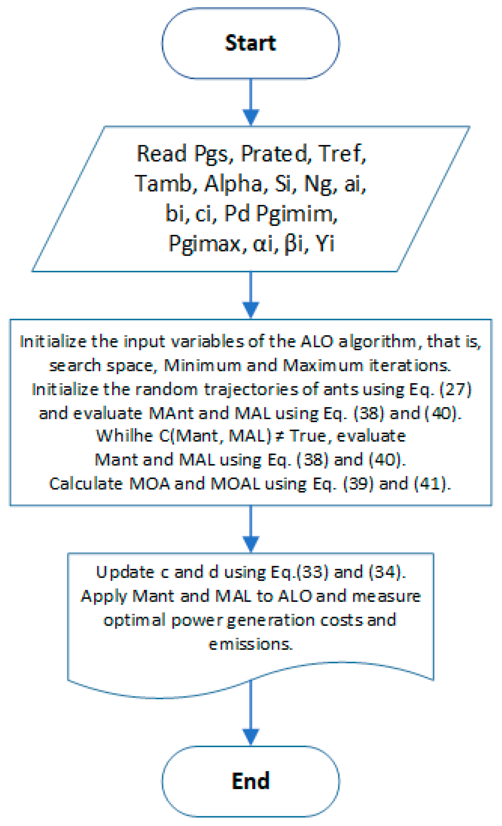
Ant lion, the optimization technique of ant lion, is a stochastic research algorithm based on a recently developed population propounded by [52] to solve problems of restricted optimization engineering issues. ALO is inspired by the lifespan of ant lions (doodlebugs), which belong to the family Myrmeleontidae and the order Neuroptera (grid of insects with wings). This technique is a free algorithm of the grid and lacks a baseline for adjustment. Because ALO is a population-based algorithm, the avoidance of ideal places is inherently high. The ALO algorithm has a high probability of solving ideal place closeness because of the random loops and roulette swivels. The pursuit of space exploration in the ALO algorithm is guaranteed by random selection of ant lions and random loops of ants all around it, and the pursuit of space exploration is guaranteed by the adaptive shrinkage limits of ant lion traps [53]:

✓

The ants random loop

✓

Building traps

✓

Ants entanglement with traps

✓

Catching preys and

✓

Traps restoration.

Adult and larval stages are both important stages of the ALO lifespan. Ant lions prey on the larval and adult phases. The larval period was based on the ALO algorithm. It digs the sand into a cone-shaped pit, following a circular path, and displaces the sand with its jaw. After the trap is built, the larva waits for its prey. The trap size differs depending on the maggots’ hungriness, ant lion, and moon size [53].

The ALO algorithm can also be optimized to issue an EELD [35,53]. This algorithm is effectively applied to solve many categories of test functions (non-modal, multi-model, and compounded). The ALO technique is converted to a fast-converted general resolution owing to the use of the roulette selection method, which is also read with optimization issues that remain discrete. With different application problems, the use of ALO technique is valid in comparison with other algorithms such as PSO, DE and DA.

As the ants transit on the pursuit space randomly to find prey, a random loop is selected to demonstrate the ant’s effort in Equation (27) [35,52,53]:

$$X\left(t\right)=\left[0, cumsum\left(2r\left(t_1\right)-1\right), cumsum\left(2r\left(t_2\right)-1\right),\dots , cumsum\left(2r\left(t_n\right)-1\right) \right]$$

(27)

where $cumsum$ computes the accumulated total, n is the maximum number of iterations, t is the current iteration, and $r\left(t_n\right)$ is the stochastic function described in Equation (28) [35,52,53]:

$$r\left(t\right)=\{\begin{array}{c}1 if rand>0.5\\ 0 if otherwise\end{array}$$

(28)

To maintain the random walks of ants inside the search space, the positions of their walks are normalized using the following min–max normalization described in Equation (29):

$$X_i^t=\frac{\left(X_i^t-a_i\right)\times \left(d_i^t-c_i^t\right)}{b_i-a_i}+c_i^t$$

(29)

where a_i and b_i are the minimum and maximum of the ith variable of random iterations, respectively, $c_i^t$ and $d_i^t$ indicate the minimum and maximum ith iteration in the tth variable, respectively.

The mathematical expression of the trapping of ants in the ant lion pits is given by Equations (30) and (31) as follows:

$$c_m^t=Ant-lio{n}_n^t-c^t$$

(30)

$$d_m^t=Ant-lio{n}_n^t-d^t$$

(31)

The fittest ant lions were selected using the roulette-wheel method. The sliding of ants into pits is given by Equations (32) and (33) [35,52,53]:

$$c^t=\frac{c^t}{I}$$

(32)

$$d^t=\frac{d^t}{I}$$

(33)

where $c^t$ is the minimum of all variables at the tth iteration, and $d^t$ the vector including the maximum of all variables at the tth iteration, and I is a ratio according to Equation (34):

$$I={10}^w \left(t/S\right)$$

(34)

where t is the current iteration, S is the maximum number of iterations, and w is a constant given by Equation (35) [54]:

$$w=\{\begin{array}{c}2 if t>0.1 S\\ 3 if t>0.5 S\\ 4 if t>0.75 S\\ 5 if t>0.9 S\\ 6 if t>0.95 S\end{array}$$

(35)

The ant lion captures the ant when it hits the rock bottom and consumes it. Subsequently, the ant needs to update its position to capture the new prey. This process is represented by Equation (36).

$$Antlio{n}_j^t=An{t}_i^t,if f\left(An{t}_i^t\right)>f\left(Antlio{n}_j^t\right)$$

(36)

On what $Antlio{n}_i^t$ indicates the position jth to the ant lion selected in the iteration, $An{t}_i^t$ displays the ant position in the iteration, and t indicates the current iteration.

Elitism was used to preserve the best solutions in each procedure. The lion ant result is treated as elite, where the technique is more apt. The elite should affect the ant at each step (random movement). For this, each ant is assigned a breeder by the roulette wheel and elite, which is given by Equation (37) [35]:

$$An{t}_i^t=\frac{R_A^t+R_B^t}{2}$$

(37)

where $R_A^t$ is the random path around the ant lion selected by the roulette method in the tth iteration, $R_B^t$ is the random trajectory around the elitism of tth e $An{t}_i^t$ indicates the positioning of the ith ant in the tth iteration.

4. Applied Procedures to Solve the CEED Problem

Actions used to solve the CEED problem:

The first step is the formation of an objective function of the CEED based on the optimization of Equations (5) and (7); the second is a power integration system, considering the IEEE-6 bus system; the third step is to apply the DA, DE, and ALO metaheuristic techniques to implement their usage guidelines; and the fourth is the progress of the technique used to obtain results from the energy system.

The CEED impacts were managed as a simultaneous multi-objective optimization problem. To solve this problem, the techniques must reduce the total cost of fuel consumption and pollutant emissions from the generating units [35,55,56].

We used three meta-heuristic techniques to compare the results obtained and evaluate which achieved the best result for the CEED problem. In the following example, details of the implementation of the ALO are provided.

Optimization steps:

Step 1.

The main agent of the ALO search, are characterized by the set of ants with random values.

Step 2.

The capacity value of each ant is evaluated using an objective function (Equation (15)) for each iteration.

Step 3.

The ants’ random paths through the search space are expected by the ant lion ant traps.

Step 4.

The position of the ants are evaluated in each iteration and the ones in the best position are relocated to capture the others.

Step 5.

The Lion ant is more agile, as it needs its position updated to catch the ant that becomes fitter.

Step 6.

An elite ant lion can affect the movement of the other ants, regardless of their displacement.

Step 7.

If a lion ant becomes better than the elite, then it is replaced by the new aptitude.

Step 8.

Steps 2 to 7 are repeated until the final parameter is satisfied.

Step 9.

The position and fitness coordinates of the elite ant lion are replicated as the best inferences for the overall optimization.

Random trajectories of the ants using Equation (27). In addition to ants, it can be assumed that ants are hidden somewhere in the search space; to save their positions and aptitude values, the following matrices are used (38)–(41) [35,52]:

$$M_{Ant}={\left[\begin{array}{ccccc}An{t}_{1,1}& An{t}_{1,2}& An{t}_{1,3}& \dots & An{t}_{1,d}\\ An{t}_{2,1}& An{t}_{2,2}& An{t}_{2,3}& \dots & An{t}_{2,d}\\ \dots & \dots & \dots & \dots & \\ An{t}_{n,1}& \dots & \cdots & \dots & An{t}_{n,d}\end{array}\right]}_{ n\times d}$$

(38)

where M_Ant is the matrix that stores each ant lion position, AL_i,j is the value of the jth dimension of the ith ant lion, n is the number of ant lions, and d is the number of variables.

To evaluate the generating units (ants), objective functions referred to in Equations (4) and (5) are used in developing the optimization and matrix (38), to keep the value of the characteristics of all generators:

$$M_{OA}=\left[\begin{array}{c}f\left(\left[An{t}_{1,1}, An{t}_{1,2}, \cdots ,An{t}_{1,d}\right]\right)\\ f\left(\left[An{t}_{2,1}, An{t}_{2,2}, \cdots , An{t}_{2,d}\right]\right)\\ ⋮\\ f\left(\left[An{t}_{n,1}, An{t}_{n,2}, \cdots , An{t}_{n,d}\right]\right)\end{array}\right]$$

(39)

where M_OA is the matrix that maintains the fitness of each ant, Ant_i,j shows the value of the jth dimension of the ith, n is the number of ants, and f is the objective function.

To optimize the cost and power generation, matrices (40) and (41) are used:

$$M_{AL}={\left[\begin{array}{ccccc}A{L}_{1,1}& A{L}_{1,2}& A{L}_{1,3}& \dots & A{L}_{1,d}\\ A{L}_{2,1}& A{L}_{2,2}& A{L}_{2,3}& \dots & A{L}_{2,d}\\ \dots & \dots & \dots & \dots & \\ A{L}_{n,1}& \dots & \cdots & \dots & A{L}_{n,d}\end{array}\right]}_{ n\times d}$$

(40)

where M_AL stores the position of each ant, AL_i,j shows the ALO proportion value j, n is the number of ants, and d is the number of variables (i.e., generators).

$$M_{OAL}=\left[\begin{array}{c}f\left(\left[A{L}_{1,1}, A{L}_{1,2}, \cdots ,A{L}_{1,d}\right]\right)\\ f\left(\left[A{L}_{2,1}, A{L}_{2,2}, \cdots , A{L}_{2,d}\right]\right)\\ ⋮\\ f\left(\left[A{L}_{n,1}, A{L}_{n,2}, \cdots , A{L}_{n,d}\right]\right)\end{array}\right]$$

(41)

where M_OAL stores the properties of each ALO, AL_i,j is the value of the jth dimension of the jth ALO, n is the number of ants, and f is the objective function of the optimization.

The number of generations of the system involving the solution that will be optimized shows the results for minimizing the costs and emissions of the contaminant gases, where it meets the constraints of Equations (8)–(13).

Equation (15) was applied to assess the performance of the CEED, although optimal costs and emissions were achieved. For inequality restrictions analogous to other techniques, the solutions achieved for any iteration are off-limits, causing the algorithm to continue until the maximum iteration and best results are obtained [57]. A flowchart of the ALO method is shown in Figure 1.

5. Case Study: IEEE 6-Units Test System and 13 Solar Plants

The proposed model satisfied 100% of the demand. For safety reasons, 80% or less of the SPPs capacity will be used; owing to the instability in energy capitation by the SPP generators, the rest of the demand will be met by TPP. In terms of the percentage of TPP to be served, optimization techniques were applied to solve the CEED problem, considering a test system with six units to meet some demand needs [8]. The selected TPP case study is composed of (six) generating units, which present fuel consumption coefficients (a, b, and c) and minimum (Pmin) and maximum (Pmax) power limits, as listed in

Table 1. Fuel cost coefficients for each thermoelectric plant generating unit. Source: [8,58].

Machine No.	a ($/MW2h)	b ($/MW/h)	c ($/h)	Pmin (MW)	Pmax (MW)
1	0.15247	38.53973	756.79886	10	125
2	0.10587	46.15916	451.32513	10	150
3	0.02803	40.39655	1049.32513	40	250
4	0.03546	38.30553	1243.5311	35	210
5	0.02111	36.32782	1658.5696	130	325
6	0.01799	38.27041	1353.27041	125	315

.

Table 2. Emission coefficients of the plants. Source: [8,58].

Machine No.	α (kg/MW2 h)	β (kg/MW h)	$\mathit{\gamma }$ (kg/h)
1	0.00419	0.32767	13.85932
2	0.00419	0.32767	13.85932
3	0.00683	−0.54551	40.2669
4	0.00683	−0.54551	40.2669
5	0.00461	−0.51116	42.89553
6	0.00461	−0.51116	42.89553

lists the emission coefficients of TPP (α, β, and $\gamma$) [58].

Table 3. Power ratings and rates per unit of SPP. Source: [8].

Plant	Prated (Mw)	Unit Rate ($/kw h)
1	20	0.22
2	25	0.23
3	25	0.23
4	30	0.24
5	30	0.24
6	35	0.25
7	35	0.26
8	40	0.27
9	40	0.27
10	40	0.28
11	40	0.28
12	40	0.28
13	40	0.28

presents the power ratings and unit costs of the various SPPs, which are estimated to be within the established range.

Table 4. Solar radiation, energy demand, and temperature for 17 July 2012. Source: [8].

Time	Global Solar Radiation (W/m2)	Power Demand (MW)	Temp. (°C)
01:00	0	965	30
02:00	0	1142	29
03:00	0	1177	28
04:00	0	1198	28
05:00	5.4	1153	28
06:00	101	1136	-
07:00	253.7	1138	29
08:00	541.2	1060	31
09:00	530.4	1155	33
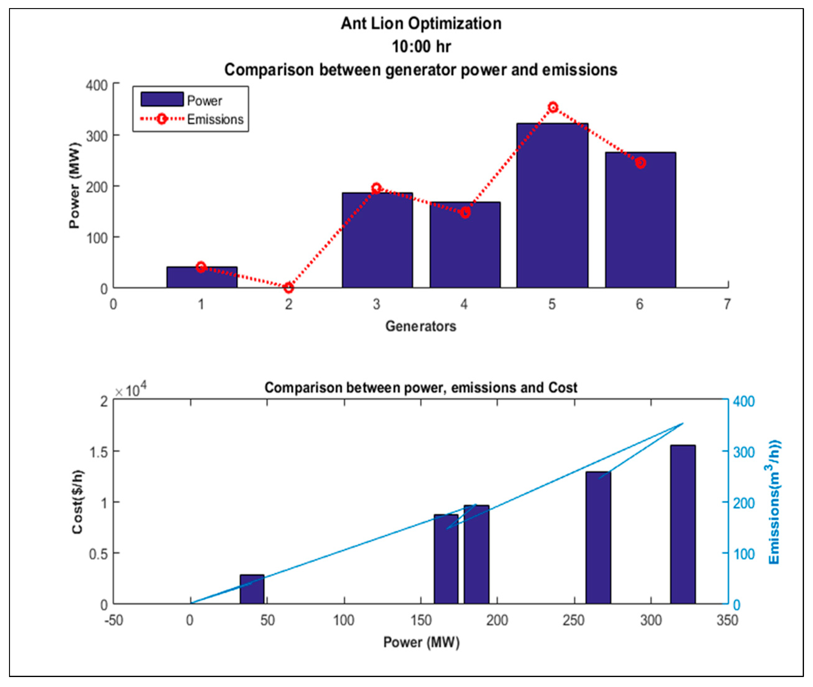
10:00	793.9	1244	34
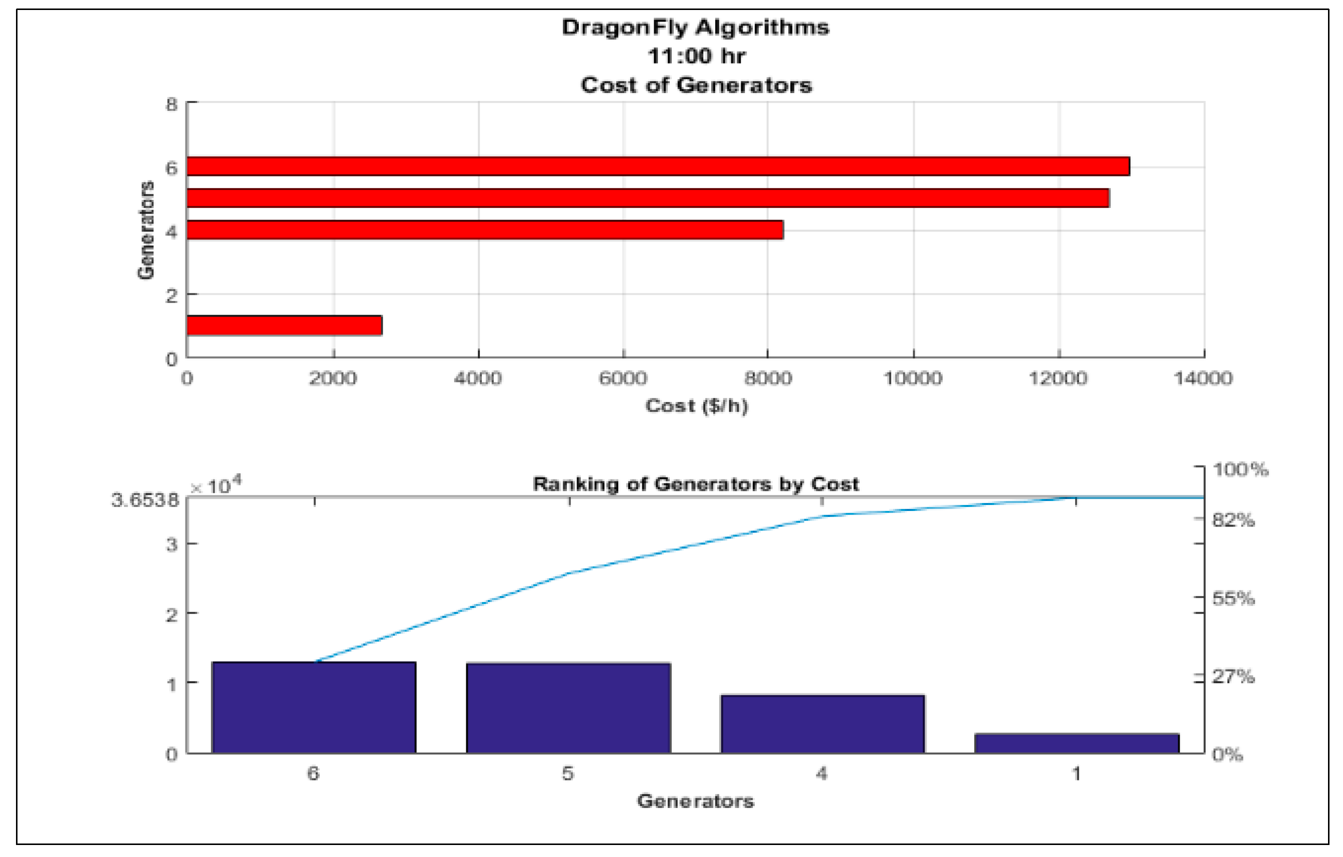
11:00	1078	1088	35
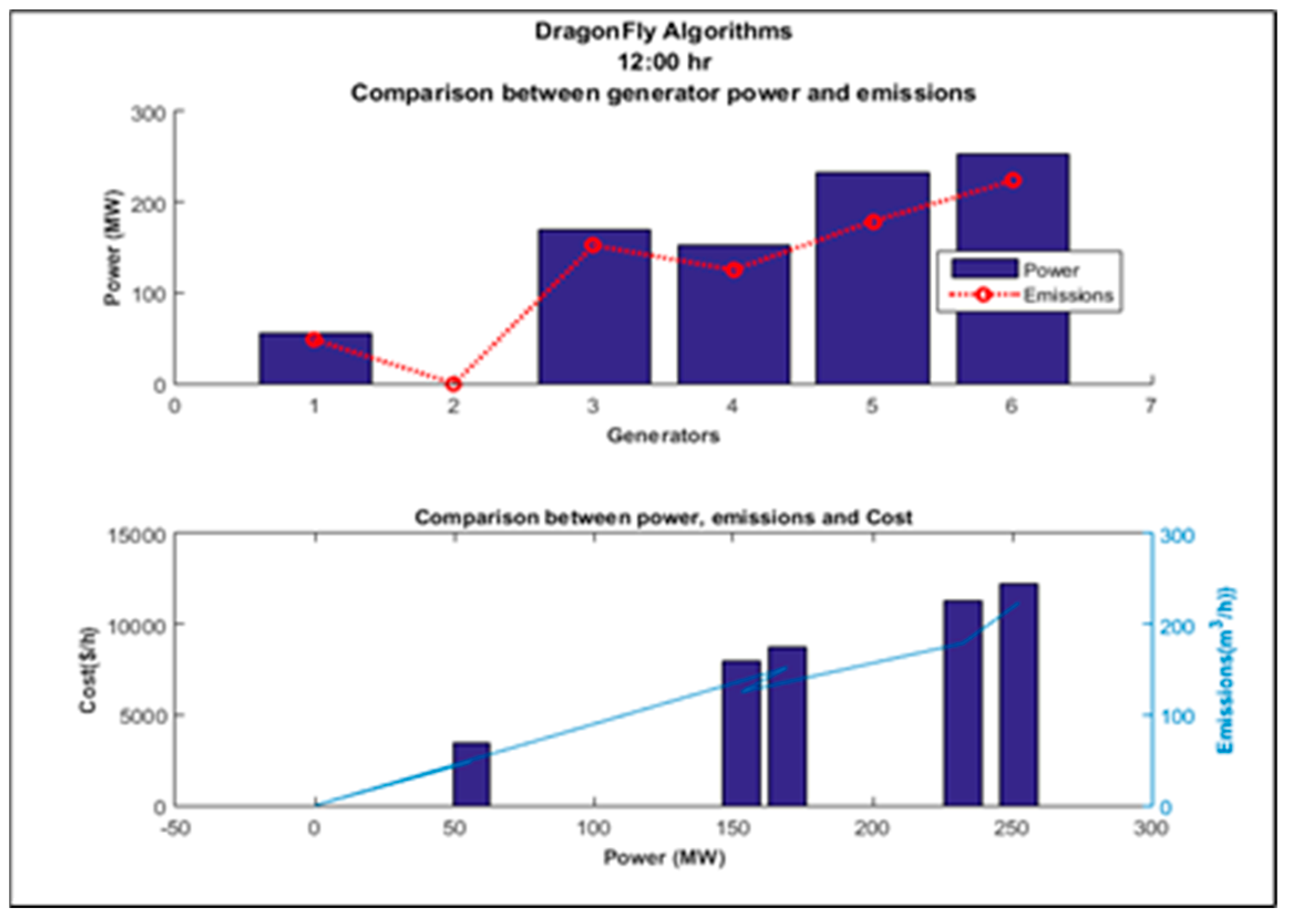
12:00	1125.6	1240	36
13:00	1013.5	1135	37
14:00	848.2	1318	37
15:00	726.7	1074	37
16:00	654	1190	38
17:00	392.9	1276	38
18:00	215.1	1154	37
19:00	385	1333	35
20:00	0	1322	34
21:00	0	1269	34
22:00	0	1139	33
23:00	0	1202	32
00:00	0	1291	-

covers global solar radiation, exactly like the temperature profiles and Islamabad charge for 17 July 2012. The solar radiation aggregated data were generated using the Geospatial Toolkit, the data related to the energy demand of the Islamabad region were taken off IESCO, and the temperature profile was obtained from [8]. Data on 17 July 2012 were selected, arbitrarily, from the only data available on that day.

6. Analysis and Discussion of Results

The results obtained from the three simulations were compared with those obtained in [8]. The proposed model was developed in a computational environment using a Core i7 machine, 8GB ram, win10 operating system with MATLAB R2015a software. The control settings used in the simulation were C1 and C2 = 2, r1 and r2 were random numbers between 0 and 1, and the maximum number of iterations was 1800, obtaining the best results for 1500, with a fixed initial population of 500 individuals considering a significant increase in computational cost for a larger number of individuals without major contributions to the results.

Table 5. The simulation presents the results with solar energy for 1244 MW demand at 10:00 a.m. Source: Authors.

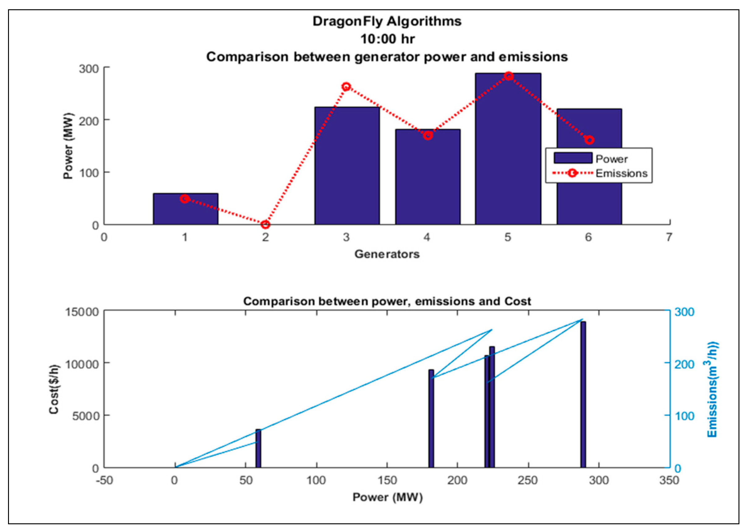
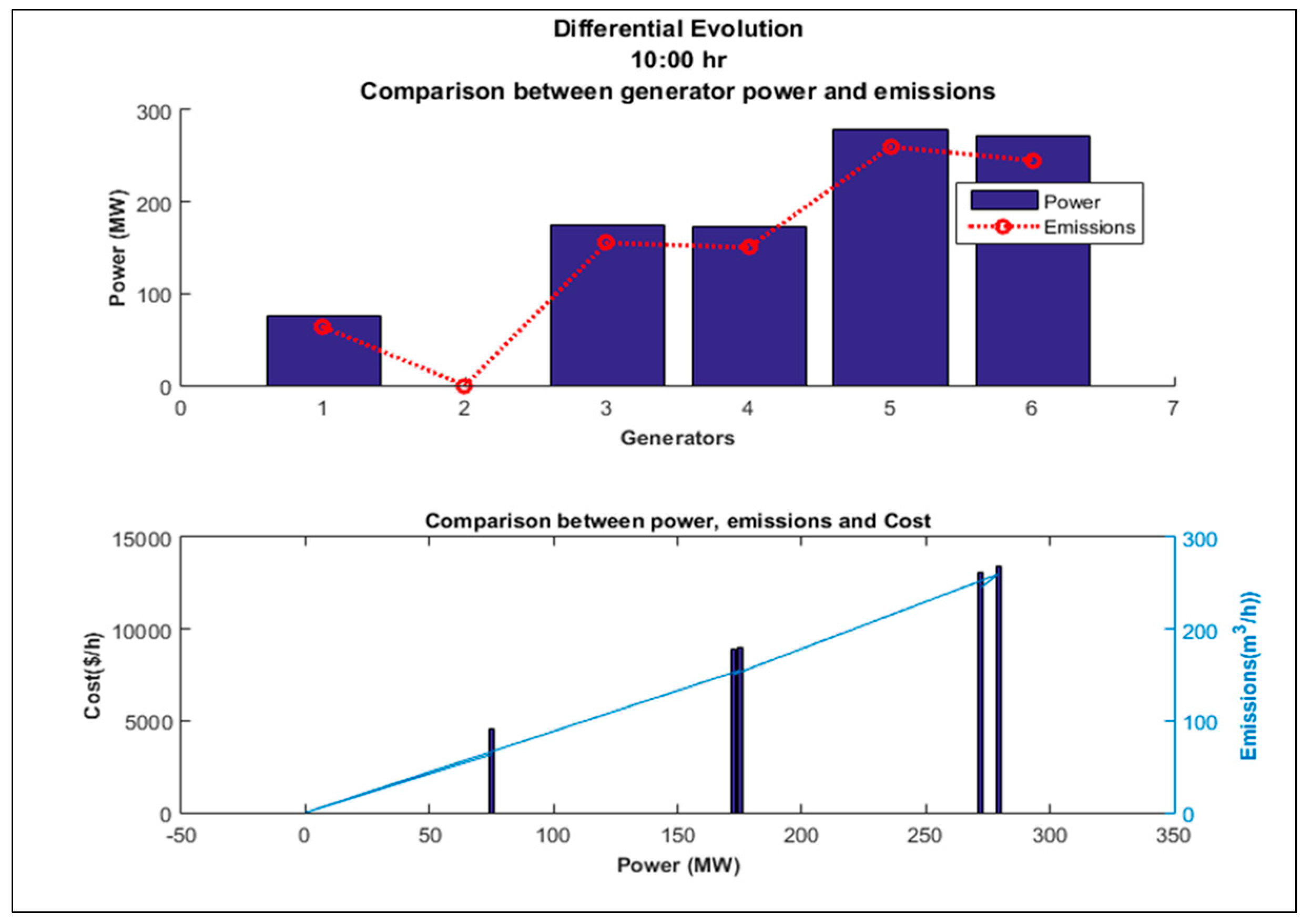
The Simulation Presents the Results for Solar Power for 1244 MW at 10:00 A.M. UG	Khan [8] PSO	ALO	DA	DE
P1 (MW)	120.4479	40.17953733	58.78230624	75.3254182
P2 (MW)	92.2947	0	0	0
P3 (MW)	155.8062	186.2565862	224.4173503	175.175433
P4 (MW)	76.4153	166.5931178	181.9118006	172.529459
P5 (MW)	257.9089	320.8753342	288.6447747	279.292715
P6 (MW)	302.2846	265.7177937	220.5766397	272.121335
Total Thermal Power (MW)	1005.1576	979.62	973.63	974.44
Solar Power share (MW)	238.825	269.644	269.644	269.644
Total Power (MW)	1243.9826	1249.27	1243.98	1244.09
Fuel cost ($/h)	52,626.00	49,337.05	49,126.17	49,027.83
Emission Reduction	19.20%	21.58%	21.69%	21.67%

presents the results obtained in the simulation at 10:00 am, which reached the total energy demand of 1244 energy.

When evaluating Table 5, it is noted that the demand of 1244 MW required for the schedule is achieved by the three optimization techniques, and the algorithm intelligently verifies the power of the six generators, shutting down with the less powerful ones. With the application of this technique, we were able to meet the demand efficiently, guaranteeing all the operating parameters of the system, and reducing fuel consumption and pollutants in the atmosphere.

We verified that the generator turned off in the simulations was the P2 UG. Even so, the energy generation did not suffer great variations, providing the stable energy generation to the system, in addition to enabling its predictive maintenance. On the other hand, the P1 UG generator presented lower power in the simulations, but in the DE technique, it exhibited better performance. In the P3 UG generator, the power variations were more notable in relation to the P1 UG generator when applied to the three techniques. The same occurs for the other P4, P5, and P6 UG generators.

We obtained the average fuel cost of the techniques (ALO, DA, and DE) compared to the Khan [8] technique, applied at 10:00 a.m. to meet the demand of 1244 MW, and achieved a reduction of approximately 6.58% corresponding to $3462.32 in the cost of fuel with the use of PV solar energy; it was possible to reduce pollutants in the atmosphere (ALO 21.58%, DA 21.69%, and DE 21.67%). The average reduction in pollutants in the atmosphere was approximately 21.64%.

Figure 2, Figure 3, Figure 4 and Figure 5 show the results of the data obtained in Table 5, which represent the values of power, emissions and fuel costs generated by the techniques (ALO, DA and DE) at 10:00 a.m. demand.

Table 6. Results show the comparison with solar energy for demand of 1088 MW at 11:00 a.m. Source: Authors.

UG	Khan [8] PSO	ALO	DA	DE
P1 (MW)	10.1062	79.3219763	41.52797	86.7820923
P2 (MW)	10	0	0	0
P3 (MW)	99.1	0	0	0
P4 (MW)	168.682	120.480886	157.301909	161.562873
P5 (MW)	235.8781	293.56174	262.569286	252.487176
P6 (MW)	246.7809	235.000594	269.032945	226.1967
Total Thermal Power (MW)	770.5472	728.37	730.43	727.03
Solar Power share (MW)	317.471	364.6572	364.6572	364.6572
Total Power (MW)	1088.0182	1093.02	1095.09	1091.69
Fuel cost ($/h)	39,426.00	36,891.78	36,537.91	36,774.07
Emission Reduction	29.18%	33.36%	33.30%	33.40%

shows the results of the comparative simulation at 11:00 a.m., reaching a total power demand of 1088 MW.

When evaluating Table 6, it is noted that the demand of 1088 MW required for the hour is achieved in the three optimization techniques, and the algorithm intelligently verifies the power of the six generators by turning off the lowest power generators. With the application of this technique, we were able to meet the demand efficiently, guaranteeing all the operating parameters of the system and reducing fuel consumption and pollutants in the atmosphere.

We verified that the generators turned off in the simulations were P2 and P3 UG; even so, the energy generation did not suffer great variations, providing the stability of the energy generation to the system, in addition to enabling predictive maintenance as the generators are turned off. On the other hand, the P1 UG generator presented lower power in the simulations, but in the DE technique, it exhibited better performance. In the P4 UG generator, the power variations were more significant in relation to the P1 UG generator when applied to the three techniques. The same occurred for the other P5 and P6 UG generators.

Obtaining the average fuel cost of the techniques (ALO, DA, and DE) compared to the Khan [8] technique, applied at 11:00 a.m. to meet the demand of 1088 MW, we were able to obtain a reduction of approximately 6.83%, which corresponds to $2691.41 in fuel cost with the use of PV solar energy. With this optimization, it was possible to reduce pollutants in the atmosphere (ALO 33.36%, DA 33.30%, and DE 33.40%) and the average reduction in pollutants in the atmosphere was approximately 33.35%.

Figure 6, Figure 7, Figure 8 and Figure 9 show the results of the data obtained in Table 6, which represent the fuel cost values generated by the techniques (ALO, DA and DE) at 11:00 a.m. demand.

Table 7. Results of comparison with solar energy for demand of 1240 MW at 12:00. Source: Authors.

UG	Khan [8] PSO	ALO	DA	DE
P1 (MW)	10.0000	60.5857502	56.0095473	64.3998993
P2 (MW)	10.2191	0	0	0
P3 (MW)	194.9316	172.74449	169.4236	155.009176
P4 (MW)	177.4014	135.063318	152.994586	151.431848
P5 (MW)	224.8683	256.93173	232.337102	246.627089
P6 (MW)	303.5647	238.005412	252.389297	243.248632
Total Thermal Power (MW)	920.9851	863.33	863.15	860.72
Solar Power share (MW)	319.1076	379.2137	379.2137	379.2137
Total Power (MW)	1240.0927	1242.54	1242.37	1239.983
Fuel cost ($/h)	46,762.00	43,635.43	43,690.57	43,393.47
Emission Reduction	25.73%	30.52%	30.52%	30.58%

presents the comparative simulation results at 12:00, reaching a total power demand of 1240 MW.

When evaluating Table 7, it is noted that the demand of 1240 MW necessary for the schedule is reached in the three optimization techniques, and the algorithm intelligently verifies the power of the six generators by turning off the less powerful ones. With the application of this technique, we were able to efficiently meet the demand, guaranteeing all the operating parameters of the system and reducing the fuel consumption and pollutants in the atmosphere.

We verified that the generator turned off in the simulations was the P2 UG. Even so, the energy generation did not suffer great variations, providing the stability of the energy generation to the system, in addition to allowing its predictive maintenance. On the other hand, the P1 UG generator presented lower power in the simulations, but in the DE technique, it exhibited better performance in relation to ALO and DA. In the P3 UG generator, the power variations were more significant in relation to the P1 UG generator when applied to the three techniques. The same was observed for the other P4, P5, and P6 UG generators.

Obtaining the average fuel cost of the techniques (ALO, DA, and DE), compared to the Khan [8] technique, applied at 12:00 to meet the demand of 1240 MW, we obtained a reduction of approximately 6.82%, which corresponds to $3188.84 in the cost of fuel, with the use of PV solar energy, it was possible to reduce pollutants in the atmosphere (ALO 30.52%, DA 30.52%, and DE 30.58%), the reduction in the average number of pollutants in the atmosphere was approximately 30.54%.

Figure 10, Figure 11, Figure 12 and Figure 13 show the results of the data obtained in Table 7, which represent the values of power, emissions and fuel costs generated by the techniques (ALO, DA and DE) at 12:00 demand.

Table 8. Results of comparison with solar energy for demand of 1135 MW at 13:00 p.m. Source: Authors.

UG	Khan [8] PSO	ALO	DA	DE
P1 (MW)	10.8593	87.5136189	76.5424528	85.1259115
P2 (MW)	118.1312	0	0	0
P3 (MW)	147.9272	0	0	0
P4 (MW)	186.3632	153.984147	179.975248	176.742446
P5 (MW)	150.7713	290.415925	290.251821	276.349213
P6 (MW)	221.0182	268.600735	261.928024	262.053767
Total Thermal Power (MW)	835.0704	800.51	808.70	800.27
Solar Power share (MW)	300.0974	340.056	340.056	340.056
Total Power (MW)	1135.1678	1140.57	1148.75	1140.33
Fuel cost ($/h)	44,136.00	40,408.16	40,689.57	40,322.38
Emission Reduction	26.44%	29.81%	29.60%	29.82%

presents the comparative results of the simulation at 13:00, reaching a total power demand of 1135 MW.

When evaluating Table 8, it was observed that the demand of 1135 MW necessary for the schedule was reached in the three optimization techniques, and the algorithm intelligently checked the power of the six generators by turning off the less powerful ones. With the application of this technique, we were able to efficiently meet the demand, guaranteeing all the operating parameters of the system and reducing the fuel consumption and pollutants in the atmosphere.

We verified that the generators turned off in the simulations were P2 and P3 UG; even so, the energy generation did not suffer great variations, providing the stability of the energy generation to the system, in addition to enabling predictive maintenance. On the other hand, the P1 UG generator presented lower power in the simulations; however, in the ALO technique, it performed better than the other techniques. In the P4 UG generator, the power variations were more significant in relation to the P1 UG generator when applied to the three techniques. The same occurred for the other P5 and P6 UG generators.

Obtaining the average fuel cost of the techniques (ALO, DA and DE), compared to the Khan [8] technique, applied at 13:00 to meet the demand of 1135 MW, we obtained a reduction of approximately 8.30% that corresponds to $3662.63 in the cost of fuel, with the use of photovoltaic solar energy, it was possible to reduce pollutants in the atmosphere (ALO 29.81%, DA 29.60% and DE 29.82%), the average reduction in pollutants in the atmosphere was approximately 29.75%.

Figure 14, Figure 15, Figure 16 and Figure 17 show the results of the data obtained in Table 8, which represent the fuel cost values generated by the techniques (ALO, DA and DE) at 13:00 p.m. demand.

Table 9. Results of comparison with solar energy for demand of 1318 MW at 14:00 p.m. SOURCE: Authors.

UG	Khan [8] PSO	ALO	DA	DE
P1 (MW)	65.2834	88.0029047	63.3546866	68.7950098
P2 (MW)	97.2893	78.8123312	74.9684444	60.8853804
P3 (MW)	250	171.876892	158.668584	172.298593
P4 (MW)	107.6407	153.785556	169.725347	169.738537
P5 (MW)	252.7949	235.599762	288.435287	289.768452
P6 (MW)	297.7576	312.66407	279.817291	275.863726
Total Thermal Power (MW)	1070.7659	1040.74	1034.97	1037.35
Solar Power share (MW)	247.1655	284.5935	284.5935	284.5935
Total Power (MW)	1317.9314	1325.34	1319.56	1321.94
Fuel cost ($/h)	55,082.00	53,803.31	52,959.36	52,691.30
Emission Reduction	18.75%	21.47%	21.57%	21.53%

presents the comparative results of the simulation at 14:00, reaching a total demand of 1318 MW of power.

When evaluating Table 9, it is noted that the demand of 1318 MW required for the schedule was reached in the three optimization techniques, and the algorithm intelligently checks the power of the six generators and is unable to turn off the generators owing to the required demand. With the application of this technique, we were able to efficiently meet the demand, guaranteeing all the operating parameters of the system and reducing the fuel consumption and pollutants in the atmosphere.

We verified that the P1 and P2 UG generators presented lower power in the simulations, but the ALO technique performed better than the other techniques. In the P3 UG generator, the power variations were more significant in relation to the P1 and P2 UG generators when applied to the three techniques. The same occurred for the other P4, P5, and P6 UG generators.

Obtaining the average fuel cost of the techniques (ALO, DA and DE), compared to the Khan [8] technique, applied at 14:00 to meet the demand of 1318 MW, we obtained a reduction of about 3.51% that corresponds to $1930.38 in the cost of fuel, with the use of PV solar energy, it was possible to reduce pollutants in the atmosphere (ALO 21.47%, DA 21.57% and DE 21.53%), the average reduction in pollutants in the atmosphere was approximately 21.52%.

Figure 18, Figure 19, Figure 20 and Figure 21 show the results of the data obtained in Table 5, which represent the values of power, emissions and fuel costs generated by the techniques (ALO, DA and DE) at 14:00 p.m. demand.

The

Table 10. Results of comparison with solar energy for demand of 1074 MW at 15:00 p.m. Source: Authors.

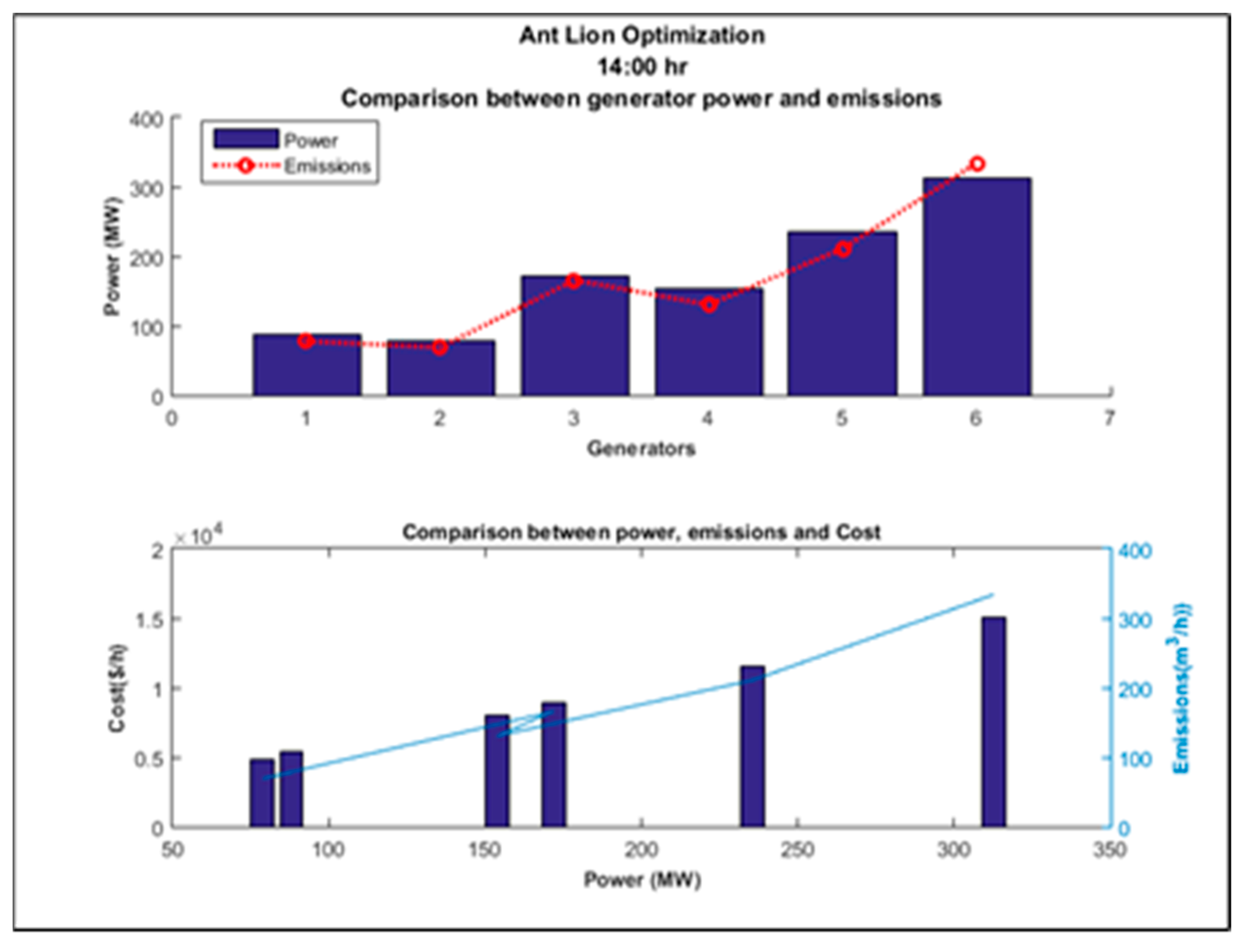
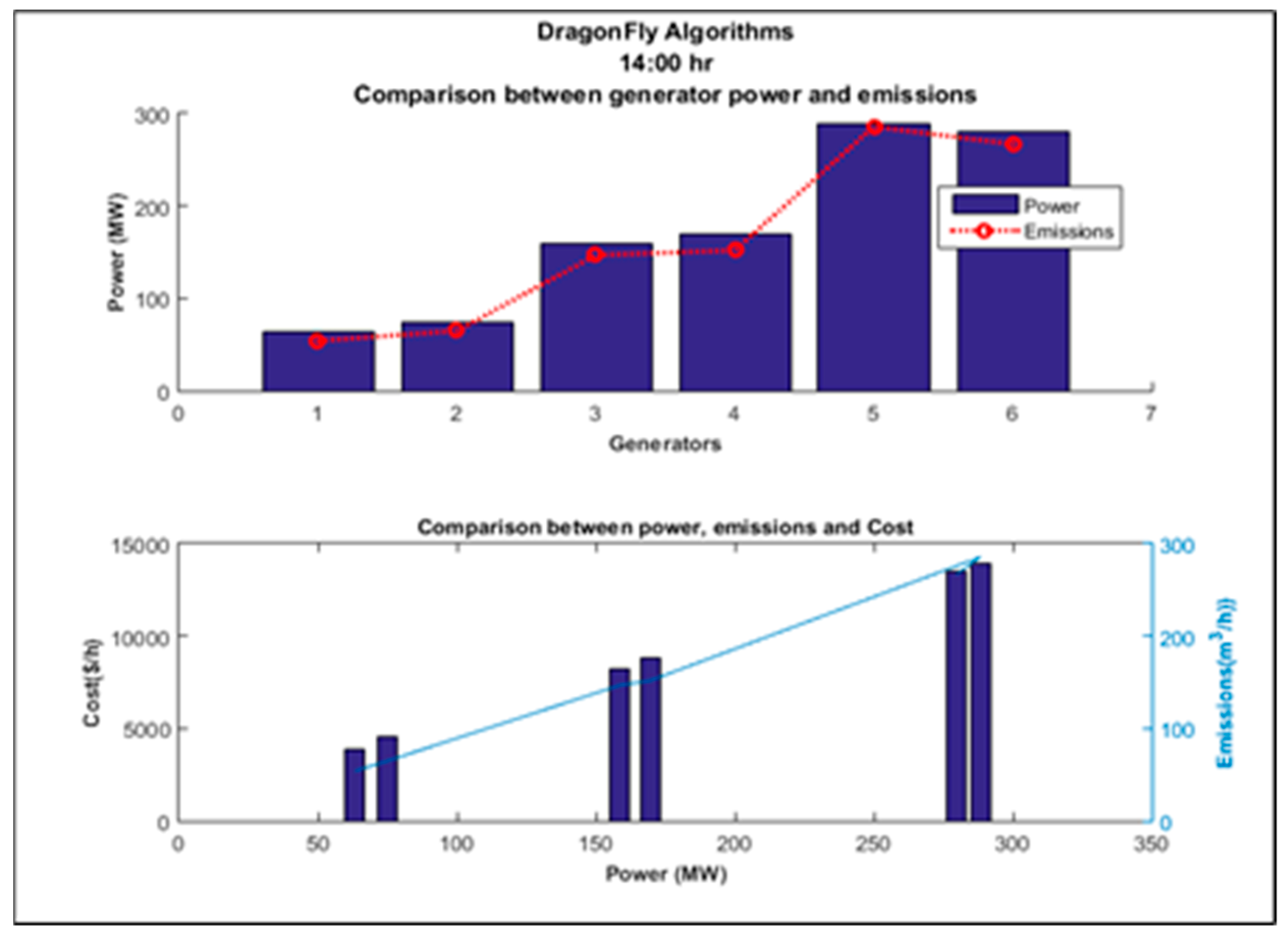
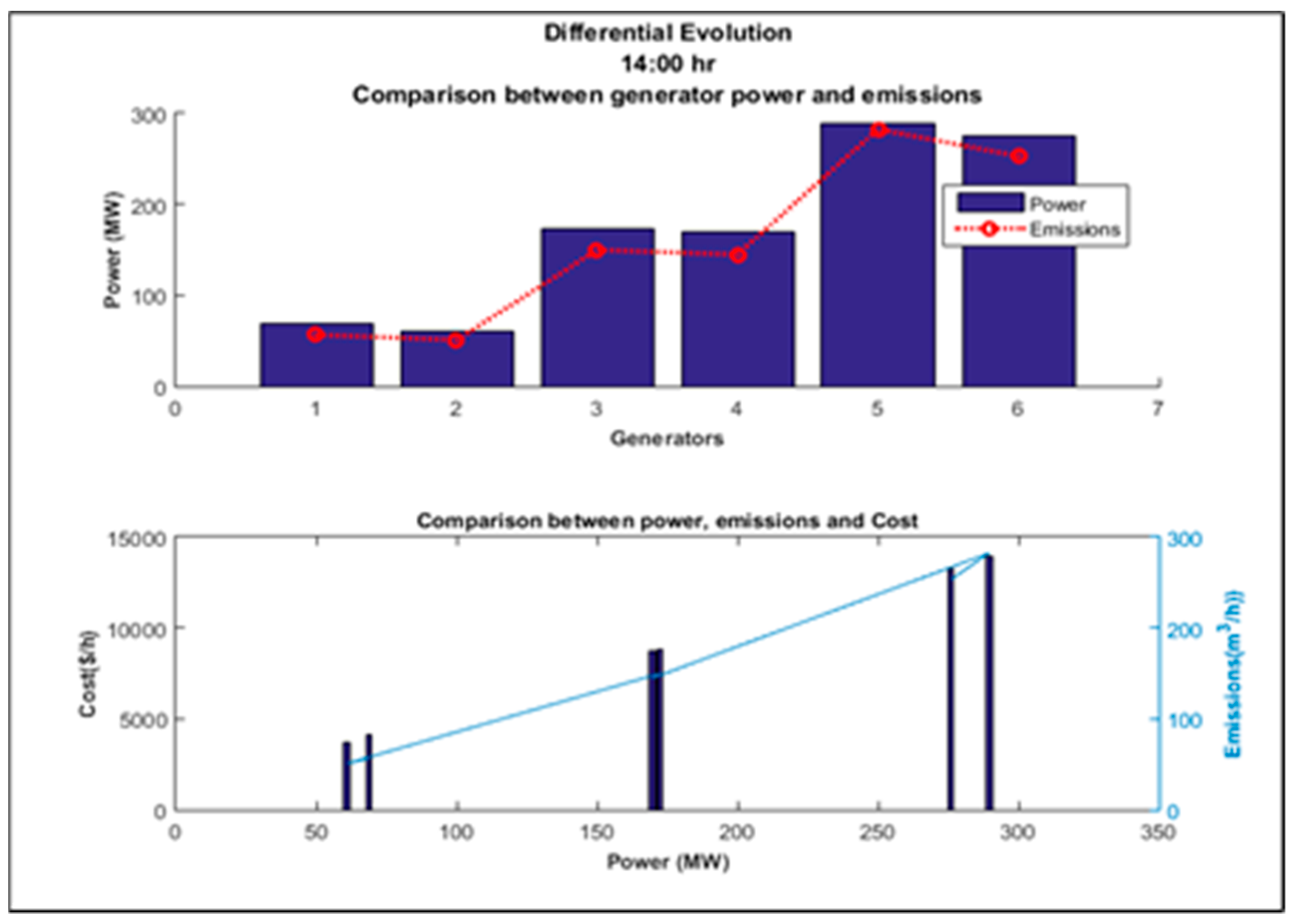
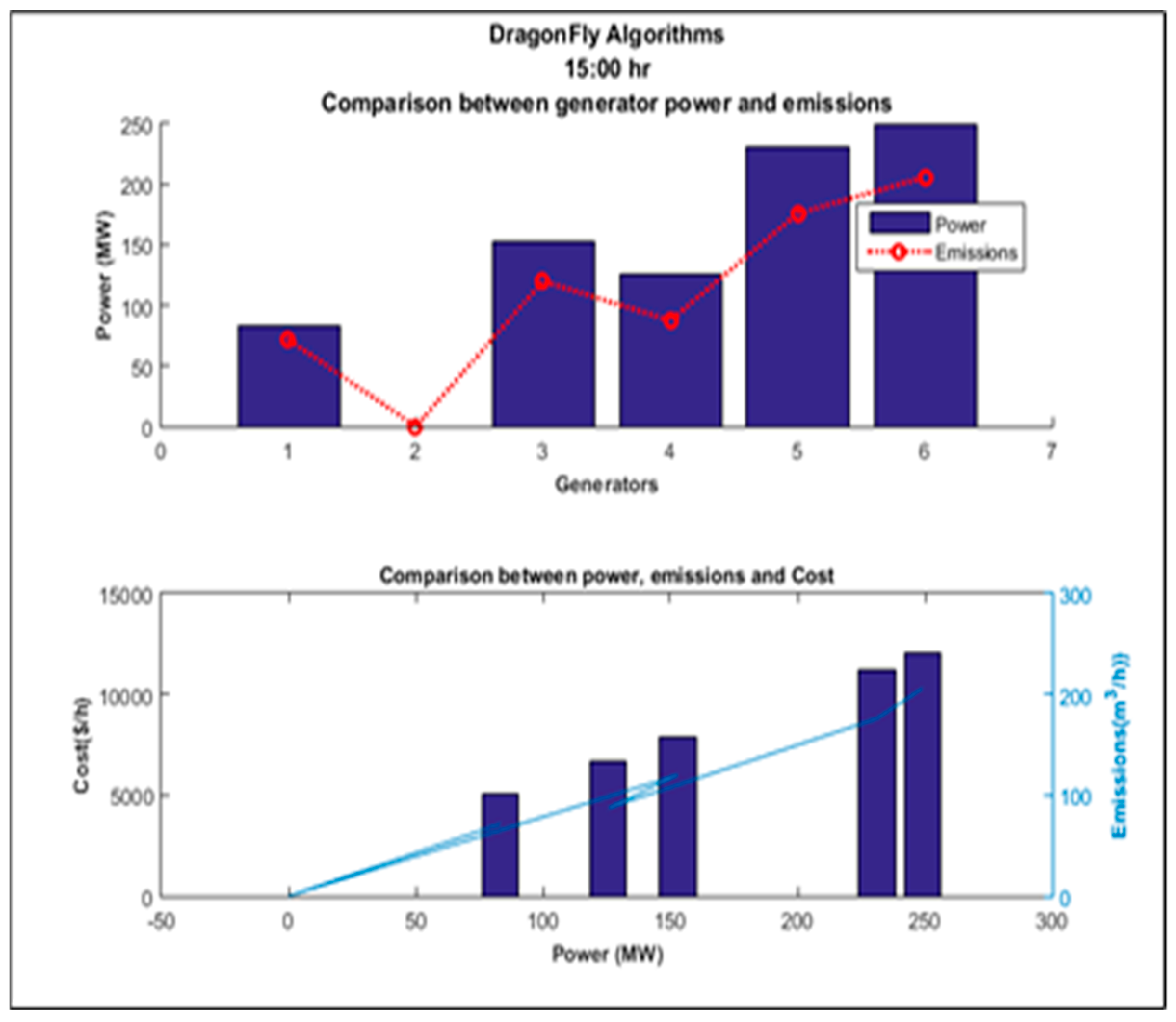
UG	Khan [8] PSO	ALO	DA	DE
P1 (MW)	82.7064	72.2365132	83.3714766	68.5854703
P2 (MW)	60.696	0	0	0
P3 (MW)	249.2579	109.101221	152.882149	146.602609
P4 (MW)	96.2554	164.950939	125.772343	143.316844
P5 (MW)	182.7257	219.94956	231.070386	239.300268
P6 (MW)	190.6486	266.531475	248.983057	232.386728
Total Thermal Power (MW)	862.29	832.77	842.08	830.19
Solar Power share (MW)	211.7604	243.827	243.827	243.827
Total Power (MW)	1074.0504	1076.60	1085.91	1074.02
Fuel cost ($/h)	45,057.00	42,554.83	42,856.77	41,985.64
Emission Reduction	19.72%	22.65%	22.45%	22.70%

presents the comparative results of the simulation at 15:00, reaching a total demand of 1074 MW of power.

From Table 10, it is observed that the demand of 1074 MW necessary for the schedule is reached in the three optimization techniques, and the algorithm intelligently checks the power of the six generators, regardless of whether it is possible to turn off the less powerful ones. With the application of this technique, we were able to efficiently meet the demand, guaranteeing all the operating parameters of the system and reducing the fuel consumption and pollutants in the atmosphere.

We verified that the generator turned off in the simulations was the P2 UG. Even so, the energy generation did not suffer great variations, providing the stability of the energy generation to the system, in addition to allowing its predictive maintenance. On the other hand, the P1 UG generator presented lower power in the simulations, but in the DA technique, it showed better performance in relation to ALO and DE. In the P3 UG generator, the power variations were more significant in relation to the P1 UG generator when applied to the three techniques. The same occurred for the other P4, P5, and P6 UG generators.

Obtaining the average fuel cost of the techniques (ALO, DA, and DE), compared to the Khan [8] technique, applied at 15:00 to meet the demand of 1074 MW, we obtained a reduction of approximately 5.75%, which corresponds to $2591.25 in the cost of fuel. With the use of PV solar energy, it was possible to reduce pollutants in the atmosphere (ALO 22.65%, DA 22.45%, and DE 22.70%), the average reduction in pollutants in the atmosphere was approximately 22.60%.

Figure 22, Figure 23, Figure 24 and Figure 25 show the results of the data obtained in Table 5, which represent the values of power, emissions and fuel costs generated by the techniques (ALO, DA and DE) at 15:00 p.m. demand.

It can be seen in the graphs of the Pareto Front figures (Cost × Emissions), for example, Figure 25, that the curves are inversely proportional, therefore, a multi-objective problem is configured.

Table 11. Comparison of total cost. SOURCE: Authors.

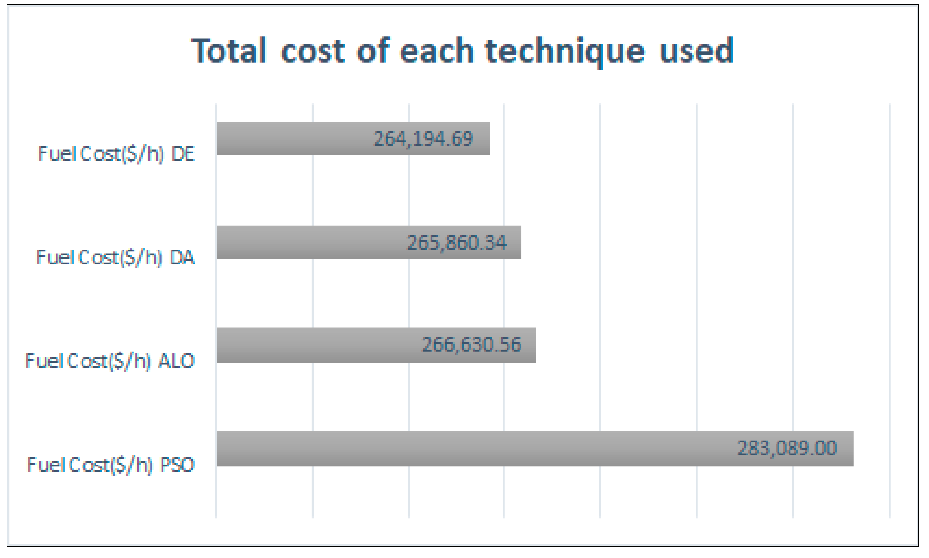
Time Hours	PSO	ALO		DA		DE
	Fuel Cost ($/h)	Fuel Cost ($/h)	Reduction %	Fuel Cost ($/h)	Reduction %	Fuel Cost ($/h)	Reduction %
10:00	52,626.00	49,337.05	6.25	49,126.17	6.65	49,027.83	6.84
11:00	39,426.00	36,891.78	6.43	36,537.91	7.33	36,774.07	7.33
12:00	46,762.00	43,635.43	6.69	43,690.57	6.57	43,393.47	7.20
13:00	44,136.00	40,408.16	8.45	40,689.57	7.81	40,322.38	8.64
14:00	55,082.00	53,803.31	2.32	52,959.36	3.85	52,691.30	4.34
15:00	45,057.00	42,554.83	5.55	42,856.77	4.88	41,985.64	6.82
Total	283,089.00	266,630.56	5.81	265,860.34	6.09	264,194.69	6.67

presents the simulated metaheuristic techniques from 10:00 a.m. to 15:00 p.m. and the results achieved by each technique. We observed that the DE technique achieved the best fuel cost reduction five times in the six simulations, DA obtained the second-best result, ALO was in third place, and obtained better results only on PSO.

The proposed algorithms maintained the generators at their optimal power to obtain better efficiency at all times. The new proposal shows that among the techniques used, the DE technique was the best, guaranteeing the reduction in fossil fuel use by 6.67%, corresponding to $18,894.31, DA reduction by 6.09%, corresponding to $17,228.66, ALO obtained the smallest reduction 5.81%, corresponding to $16,458.44, the results were compared with the PSO technique.

During the simulations, the greatest reduction occurred at 13:00 p.m. with 8.64% and the smallest reduction occurred at 14:00 p.m. with 4.34%.

Figure 26 shows the results of the data obtained in Table 11, in which the general fuel cost obtained between 10:00 a.m. and 15:00 p.m., achieves the best performance (cost reduction) with the DE technique.

7. Conclusions

Aiming to reliably show alternatives to supply the generation of energy has been one of the research objectives for several years. Thus, this work is a viable solution for sustainable clean energy, responsible for solving the problem of optimization of CEED using a hybrid system composed of TPP and photovoltaic generation. By choosing photovoltaic plants to meet the energy demand, a cleaner production with less environmental impact was achieved, contributing to a decrease in contaminants released into the atmosphere. The new method intelligently checks the capacity of the generators in use and, depending on the demand requested for the time, switches off the least efficient thermal generator. With the application of these techniques, it is possible to meet the energy demand efficiently, guarantee all the operating parameters of the system, reduce fuel costs, and reduce pollutant emissions. Thus, the application of metaheuristics to optimize CEED proved to be efficient and reliable with excellent results. The new proposal shows that among the techniques used, DE was the method that presented the best results, guaranteeing a reduction in the use of fossil fuel by 6.67%, corresponding to $18,894.31. The DA also obtained a reduction of 6.09% corresponding to $17,228.66, while ALO obtained 5.81% corresponding to $16,458.44. These results were compared with the results of Khan simulations, which used PSO. The results achieved using the ALO, DA, and DE techniques demonstrate the robustness of the application of these algorithms in optimization problems.

References

- Panigrahi, T.K.; Sahoo, A.K.; Behera, A. A review on application of various heuristic techniques to combined economic and emission dispatch in a modern power system scenario. Energy Procedia 2017, 138, 458–463. [Google Scholar] [CrossRef]
- Younes, Z.; Alhamrouni, I.; Mekhilef, S.; Reyasudin, M. A memory-based gravitational search algorithm for solving economic dispatch problem in micro-grid. Ain. Shams. Eng. J. 2021, 12, 1985–1994. [Google Scholar] [CrossRef]
- Zhang, B.; Sudhoff, S.; Pekarek, S.; Swanson, R.; Flicker, J.; Neely, J.; Delhotal, J.; Kaplar, R. Prediction of Pareto-Optimal Performance Improvements in A Power Conversion System Using GaN Devices. In Proceedings of the 2017 IEEE 5th Workshop on Wide Bandgap Power Devices and Applications (WiPDA), Santa Ana Pueblo, NM, USA, 30 October–1 November 2017; pp. 80–86. [Google Scholar] [CrossRef]
- Goyal, S.K.; Singh, J.; Saraswat, A.; Kanwar, N.; Shrivastava, M.; Mahela, O.P. Economic Load Dispatch with Emission and Line Constraints using Biogeography Based Optimization Technique. In Proceedings of the 2020 International Conference on Intelligent Engineering and Management (ICIEM), London, UK, 17–19 June 2020; pp. 471–476. [Google Scholar] [CrossRef]
- Bai, Y.; Wu, X.; Xia, A. An enhanced multi-objective differential evolution algorithm for dynamic environmental economic dispatch of power system with wind power. Energy Sci. Eng. 2020, 9, 316–329. [Google Scholar] [CrossRef]
- Sarfi, V.; Niazazari, I.; Livani, H. Multiobjective Fireworks Optimization Framework for Economic Emission Dispatch in Microgrid. In Proceedings of the 2016 North American Power Symposium (NAPS), Denver, CO, USA, 18–20 September 2016; pp. 1–6. [Google Scholar] [CrossRef]
- Dey, B.; Bhattacharyya, B.; Raj, S.; Babu, R. Economic emission dispatch on unit commitment-based microgrid system considering wind and load uncertainty using hybrid MGWOSCACSA. J. Electr. Syst. Inf. Technol. 2020, 7, 1–26. [Google Scholar] [CrossRef]
- Khan, N.A.; Awan, A.B.; Mahmood, A.; Razzaq, S.; Zafar, A.; Sidhu, G.A.S. Combined emission economic dispatch of power system including solar photo voltaic generation. Energy Convers. Manag. 2015, 92, 82–91. [Google Scholar] [CrossRef]
- Ma, H.; Yang, Z.; You, P.; Fei, M. Multi-objective biogeography-based optimization for dynamic economic emission load dispatch considering plug-in electric vehicles charging. Energy 2017, 135, 101–111. [Google Scholar] [CrossRef]
- Meziane, M.A.; Mouloudi, Y.; Draoui, A. Comparative study of the price penalty factors approaches for Bi-objective dispatch problem via PSO. Int. J. Electr. Comput. Eng. IJECE 2020, 10, 3343–3349. [Google Scholar] [CrossRef]
- Al-Betar, M.A.; Awadallah, M.A.; Krishan, M.M. A non-convex economic load dispatch problem with valve loading effect using a hybrid grey wolf optimizer. Neural Comput. Appl. 2019, 32, 12127–12154. [Google Scholar] [CrossRef]
- Elsayed, W.; El-Saadany, E.F.; Zeineldin, H.H.; Al-Sumaiti, A.S. Fast initialization methods for the nonconvex economic dispatch problem. Energy 2020, 201, 117635. [Google Scholar] [CrossRef]
- Zheng, M.; Wang, X.; Meinrenken, C.J.; Ding, Y. Economic and environmental benefits of coordinating dispatch among distributed electricity storage. Appl. Energy 2018, 210, 842–855. [Google Scholar] [CrossRef]
- Qin, Q.; Cheng, S.; Chu, X.; Lei, X.; Shi, Y. Solving non-convex/non-smooth economic load dispatch problems via an enhanced particle swarm optimization. Appl. Soft Comput. 2017, 59, 229–242. [Google Scholar] [CrossRef]
- Sharifi, S.; Sedaghat, M.; Farhadi, P.; Ghadimi, N.; Taheri, B. Environmental economic dispatch using improved artificial bee colony algorithm. Evol. Syst. 2017, 8, 233–242. [Google Scholar] [CrossRef]
- Reddy, A.S. Optimization of distribution network reconfiguration using dragonfly algorithm. J. Electr. Eng. 2016, 16, 10. [Google Scholar]
- Yıldız, B.S.; Yıldız, A.R. The Harris hawks optimization algorithm, salp swarm algorithm, grasshopper optimization algorithm and dragonfly algorithm for structural design optimization of vehicle components. Mater. Test. 2019, 61, 744–748. [Google Scholar] [CrossRef]
- dos Santos, E.S.; Nunes, M.V.A.; Júnior, J.D.A.B.; Nascimento, M.H.R.; Leite, J.C.; de Alencar, D.B.; de Freitas, C.A.O. Efficient use of the Generators for the Environmental Economic Dispatch from the energy system, including solar photovoltaic generation. Int. J. Innov. Educ. Res. 2021, 9, 9–34. [Google Scholar] [CrossRef]
- Qin, H.; Fan, P.; Tang, H.; Huang, P.; Fang, B.; Pan, S. An effective hybrid discrete grey wolf optimizer for the casting production scheduling problem with multi-objective and multi-constraint. Comput. Ind. Eng. 2019, 128, 458–476. [Google Scholar] [CrossRef]
- Santra, D.; Mukherjee, A.; Sarker, K.; Mondal, S. Dynamic economic dispatch using hybrid metaheuristics. J. Electr. Syst. Inf. Technol. 2020, 7, 1–30. [Google Scholar] [CrossRef] [Green Version]
- Nascimento, M.H.R.; Junior, J.D.A.B.; De Freitas, C.A.O.; Moraes, N.M.; Leite, J.C. Analysis of the solution for the economic load dispatch by different mathematical methods and genetic algorithms: Case Study. ITEGAM-JETIA 2018, 4, 5–13. [Google Scholar] [CrossRef]
- Muhsen, D.H.; Nabil, M.; Haider, H.T.; Khatib, T. A novel method for sizing of standalone photovoltaic system using multi-objective differential evolution algorithm and hybrid multi-criteria decision making methods. Energy 2019, 174, 1158–1175. [Google Scholar] [CrossRef]
- Kuk, J.N.; Gonçalves, R.A.; Pavelski, L.M.; Venske, S.M.G.S.; de Almeida, C.P.; Pozo, A.T.R. An empirical analysis of constraint handling on evolutionary multi-objective algorithms for the Environmental/Economic Load Dispatch problem. Expert Syst. Appl. 2020, 165, 113774. [Google Scholar] [CrossRef]
- Bora, T.C.; Mariani, V.C.; Coelho, L.D.S. Multi-objective optimization of the environmental-economic dispatch with reinforcement learning based on non-dominated sorting genetic algorithm. Appl. Therm. Eng. 2019, 146, 688–700. [Google Scholar] [CrossRef]
- Moraes, N.M.; Bezerra, U.H.; Moya Rodriguez, J.L.; Nascimento, M.H.R.; Leite, J.C. A new approach to economic-emission load dispatch using NSGA II. Case study. Int. Trans. Electr. Energy Syst. 2018, 28, e2626. [Google Scholar] [CrossRef]
- Ogunmodede, O.; Anderson, K.; Cutler, D.; Newman, A. Optimizing design and dispatch of a renewable energy system. Appl. Energy 2021, 287, 116527. [Google Scholar] [CrossRef]
- Bustos, C.; Watts, D.; Olivares, D. The evolution over time of Distributed Energy Resource’s penetration: A robust framework to assess the future impact of prosumage under different tariff designs. Appl. Energy 2019, 256, 113903. [Google Scholar] [CrossRef]
- Adam, S.P.; Alexandropoulos, S.-A.N.; Pardalos, P.M.; Vrahatis, M.N. No Free Lunch Theorem: A Review. In Approximation and Optimization; Springer International Publishing: Cham, Switzerland, 2019; pp. 57–82. [Google Scholar] [CrossRef]
- Abido, M. A niched Pareto genetic algorithm for multiobjective environmental/economic dispatch. Int. J. Electr. Power Energy Syst. 2003, 25, 97–105. [Google Scholar] [CrossRef]
- Wu, L.; Wang, Y.; Yuan, X.; Zhou, S. Environmental/economic power dispatch problem using multi-objective differential evolution algorithm. Electr. Power Syst. Res. 2010, 80, 1171–1181. [Google Scholar] [CrossRef]
- Mohamed, F.A.; Koivo, H.N. Online management of microgrid with battery storage using multiobjective optimization. In Proceedings of the International Conference on Power Engineering, Energy and Electrical Drives, Setubal, Portugal, 12–14 April 2007; pp. 231–236. [Google Scholar]
- Cervantes Rodriguez, C.R. Mecanismos Regulatorios, Tarifarios E Economicos Na Geração Distribuida: O Caso Dos Sistemas Fotovoltaticos Conectados a Rede. 2002. Available online: http://repositorio.unicamp.br/jspui/handle/REPOSIP/264941 (accessed on 14 March 2022).
- Basu, M. Economic environmental dispatch using multi-objective differential evolution. Appl. Soft Comput. 2011, 11, 2845–2853. [Google Scholar] [CrossRef]
- Deb, S.; Abdelminaam, D.S.; Said, M.; Houssein, E.H. Recent Methodology-Based Gradient-Based Optimizer for Economic Load Dispatch Problem. IEEE Access 2021, 9, 44322–44338. [Google Scholar] [CrossRef]
- Kamboj, V.K.; Bhadoria, A.; Bath, S.K. Solution of non-convex economic load dispatch problem for small-scale power systems using ant lion optimizer. Neural Comput. Appl. 2017, 28, 2181–2192. [Google Scholar] [CrossRef]
- Brini, S.; Abdallah, H.H.; Ouali, A. Economic dispatch for power system included wind and solar thermal energy. Leonardo J. Sci. 2009, 14, 204–220. [Google Scholar]
- Nwulu, N.; Xia, X. Multi-objective dynamic economic emission dispatch of electric power generation integrated with game theory based demand response programs. Energy Convers. Manag. 2015, 89, 963–974. [Google Scholar] [CrossRef]
- Wang, L.; Singh, C. Environmental/economic power dispatch using a fuzzified multi-objective particle swarm optimization algorithm. Electr. Power Syst. Res. 2007, 77, 1654–1664. [Google Scholar] [CrossRef]
- Huang, W.-T.; Yao, K.-C.; Chen, M.-K.; Wang, F.-Y.; Zhu, C.-H.; Chang, Y.-R.; Lee, Y.-D.; Ho, Y.-H. Derivation and Application of a New Transmission Loss Formula for Power System Economic Dispatch. Energies 2018, 11, 417. [Google Scholar] [CrossRef] [Green Version]
- Afandi, A.N. Thunderstorm algorithm for assessing thermal power plants of the integrated power system operation with an environmental requirement. Int. J. Eng. Technol. 2016, 8, 1102–1111. [Google Scholar]
- Nascimento, M.H.R.; Nunes, M.V.A.; Rodríguez, J.L.M.; Leite, J.C. A new solution to the economical load dispatch of power plants and optimization using differential evolution. Electr. Eng. 2017, 99, 561–571. [Google Scholar] [CrossRef]
- Dhamanda, A.; Dutt, A.; Prakash, S.; Bhardwaj, A.K. A traditional approach to solve economic load dispatch problem of thermal generating unit using MATLAB programming. Int. J. Eng. Res. Technol. 2013, 2, IJERTV2IS90218. [Google Scholar]
- Wolpert, D.H.; Macready, W.G. No free lunch theorems for optimization. IEEE Trans. Evol. Comput. 1997, 1, 67–82. [Google Scholar] [CrossRef] [Green Version]
- Mirjalili, S. Dragonfly algorithm: A new meta-heuristic optimization technique for solving single-objective, discrete, and multi-objective problems. Neural Comput. Appl. 2016, 27, 1053–1073. [Google Scholar] [CrossRef]
- Das, D.; Bhattacharya, A.; Ray, R.N. Dragonfly Algorithm for solving probabilistic Economic Load Dispatch problems. Neural Comput. Appl. 2020, 32, 3029–3045. [Google Scholar] [CrossRef]
- Meraihi, Y.; Ramdane-Cherif, A.; Acheli, D.; Mahseur, M. Dragonfly algorithm: A comprehensive review and applications. Neural Comput. Appl. 2020, 32, 16625–16646. [Google Scholar] [CrossRef]
- Reynolds, C.W. Flocks, herds and schools: A distributed behavioral model. In Proceedings of the 14th annual conference on Computer graphics and interactive techniques, Anaheim, CA, USA, 27–31 July 1987; pp. 25–34. [Google Scholar]
- Storn, R. Differrential evolution-a simple and efficient adaptive scheme for global optimization over continuous spaces. Tech. Rep. Int. Comput. Sci. Inst. 1995, 11. Available online: http://www.icsi.berkeley.edu/ftp/global/pub/techreports/1995/tr-95-012.pdf (accessed on 14 March 2022).
- Storn, R.; Price, K. Differential evolution–a simple and efficient heuristic for global optimization over continuous spaces. J. Glob. Optim. 1997, 11, 341–359. [Google Scholar] [CrossRef]
- Roque, C.; Martins, P. Differential evolution for optimization of functionally graded beams. Compos. Struct. 2015, 133, 1191–1197. [Google Scholar] [CrossRef]
- Reddy, A.S.; Vaisakh, K. Shuffled differential evolution for large scale economic dispatch. Electr. Power Syst. Res. 2013, 96, 237–245. [Google Scholar] [CrossRef]
- Mirjalili, S. The Ant Lion Optimizer. Adv. Eng. Softw. 2015, 83, 80–98. [Google Scholar] [CrossRef]
- Mirjalili, S.; Jangir, P.; Saremi, S. Multi-objective ant lion optimizer: A multi-objective optimization algorithm for solving engineering problems. Appl. Intell. 2017, 46, 79–95. [Google Scholar] [CrossRef]
- Raju, M.; Saikia, L.C.; Sinha, N. Automatic generation control of a multi-area system using ant lion optimizer algorithm based PID plus second order derivative controller. Int. J. Electr. Power Energy Syst. 2016, 80, 52–63. [Google Scholar] [CrossRef]
- Refai, A.; Ebeed, M.; Kamel, S. Combined Economic and Emission Dispatch Analysis Using Lightning Attachment Procedure Optimizer. In Proceedings of the 2019 21st International Middle East Power Systems Conference (MEPCON), Cairo, Egypt, 17–19 December 2019. [Google Scholar] [CrossRef]
- Mohammed, A.S.; Murphy, G.V.; Ndoye, M. A PSO Based Control Strategy for Combined Emission Economic Dispatch with Integrated Renewables. In Proceedings of the 52nd North American Power Symposium (NAPS), Tempe, AZ, USA, 11–14 April 2021; pp. 1–5. [Google Scholar] [CrossRef]
- Trivedi, I.N.; Jangir, P.; Parmar, S.A. Optimal power flow with enhancement of voltage stability and reduction of power loss using ant-lion optimizer. Cogent Eng. 2016, 3, 1208942. [Google Scholar] [CrossRef]
- Manteaw, E.D.; Odero, N.A. Combined economic and emission dispatch solution using ABC_PSO hybrid algorithm with valve point loading effect. Int. J. Sci. Res. Publ. 2012, 2, 1–9. [Google Scholar]