A Solar Dually PVT Driven Direct Expansion Heat Pump One-Year Field Operation Results at Continental Climate

Abstract

The high energy-consuming building sector needs to meet both electricity and heat demands. In a nearly zero energy building scenario, most of the consumed energy would be generated locally by means of renewable solutions that nowadays seem not to provide an attractive performance or cost-competitiveness. Solar-based technologies tend to be the most promising ones, but for high densely populated areas, the usual photovoltaic or thermal single approaches may not be efficient enough. The current work is focused on the analysis of the dual use of the solar resource by means of hybrid PVT collectors and their smart combination with direct expansion heat pumps through predictive control strategies. To that end, a system was developed, installed in a real-use single-family house at a continental climate for domestic hot water application, operated and monitored for one entire year. The average day indicator results show 83% renewable energy share, 220% self-sufficiency ratio, 41% heat pump self-consumption and 46% of the solar fraction.

1. Introduction

Global energy consumption is projected to return quickly to pre-pandemic levels [1]. The reference for 2020 was around 600 quadrillion British thermal units with a 50% estimated increase by 2050 driven by non-OECD economic growth and population. The European Commission states [2] that buildings are responsible for 40% of the energy consumption and 36% of CO₂ emissions, and pretends to reduce their impact through different actions. Most of those buildings need to meet both electricity and heat demands, for domestic hot water (DHW) and space heating/cooling (H&C). In the close, nearly zero energy building (nZEB) scenario, most of the consumed energy would need to be generated locally by means of renewable resources. Unfortunately, current renewable solutions seem not to provide an integral, simultaneous and local solution to this need, ensuring energy supply guarantee and cost-competitiveness.

However, solar energy is available all over the face of the earth. Thus, buildings should try to take higher value from every beam of light reaching their envelopes. Today, photovoltaics (PV), and in the past, solar thermal (ST) applications, are becoming widely used for built environment on-site generation. Nevertheless, for high densely populated and shadow restricted areas, these kind of single approaches are not enough to satisfy building energy needs. Detailed analysis of solar resources in built environments shows that not only roofs but also façades should be considered with higher efficiency solar conversion devices such as PVT [3].

Harnessing solar energy should be a must for new and refurbished buildings [4,5,6], but when the sun is not shining and energy stores are empty, solar base solutions always require back-up systems, which reduces their competitiveness. The electrical grid makes things easier for loads, but thermal needs are still highly fossil fuel-dependent in a great part of Europe [7]. However, heat pumps (HP) seem a promising technology for a reduction in building thermal comfort-related CO₂ emissions and enable the use of the electrical infrastructure to use them as a back-up source [8]. Therefore, if solar and HP are individually suitable for electricity and heat generation, merging them in a unique hybrid system will enable obtaining even higher benefits [9,10,11]. Anyway, it is usually hard to inter-compare technologies and quantify those real benefits to simply conclude which one shows overall greater performance. Thus, within the current work, an experimental approach is proposed to shed some light on the real field performance of such systems.

1.1. PVT Dually Coupled HP Technology

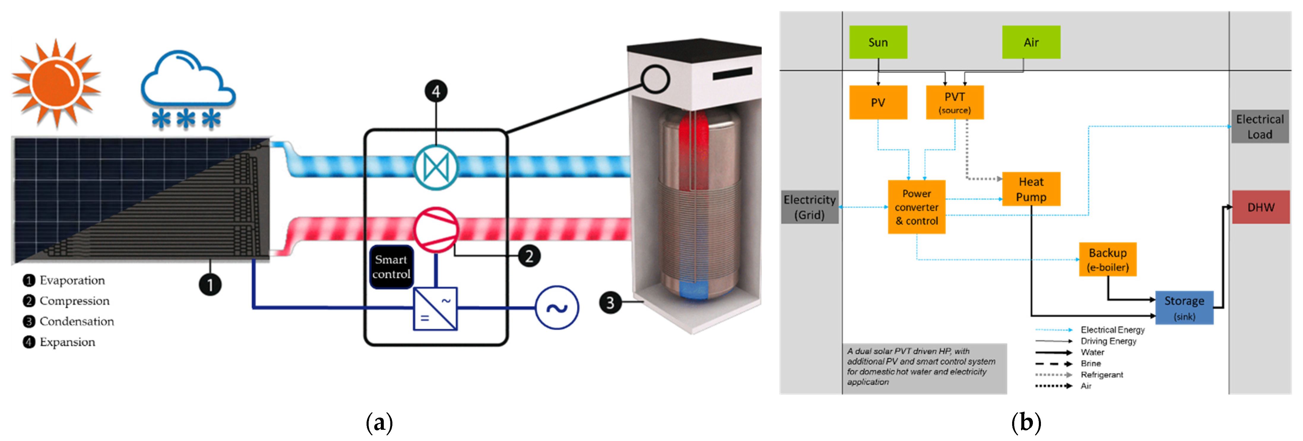
The proposed solution is a solar hybrid PVT dually coupled HP. It is a fully integrated system comprising an unglazed hybrid solar collector, a direct expansion solar assisted HP (DX-saHP) and an overall system control (Figure 1). The base of the technology has been widely studied before by different research groups for comparative analysis [12,13] and experimental studies [14,15]. The union of PV and solar thermodynamic technologies in one collector enables simultaneous electricity and heat generation and in a kind of symbiosis both technologies work optimally without mismatching the other’s performance [16], as occurs in conventional PVT where a trade-off between the thermal and electric performance is needed. Thus, the dually assisted HP significantly increases the total annual use of the solar resource while primary energy consumption is reduced.

1.2. Solution Innovations

The proposed solution incorporates innovations focusing on the main critical elements impacting the entire system’s cost-performance.

1.2.1. PVT Collector

Deep research has been carried out during recent decades on solar hybrid PVT collectors [19] and their integration at a system level [20]. The last advancements are continuously presented [21,22] and future trends are discussed [23,24] by the scientific community. In parallel, a wide set of commercial products are available [25,26,27,28,29], covering almost all different types of collectors [30] and applications [31], but the cost is significantly linked to the thermal efficiency [32,33]. However, for HP-based systems the cold side temperature is not required to be close to the application one. Thus, directly PVT coupled HP solutions could benefit from a non-high temperature collector field thermal output while ensuring proper operation [34], even just by driving the HP with PVT thermal contribution [35].

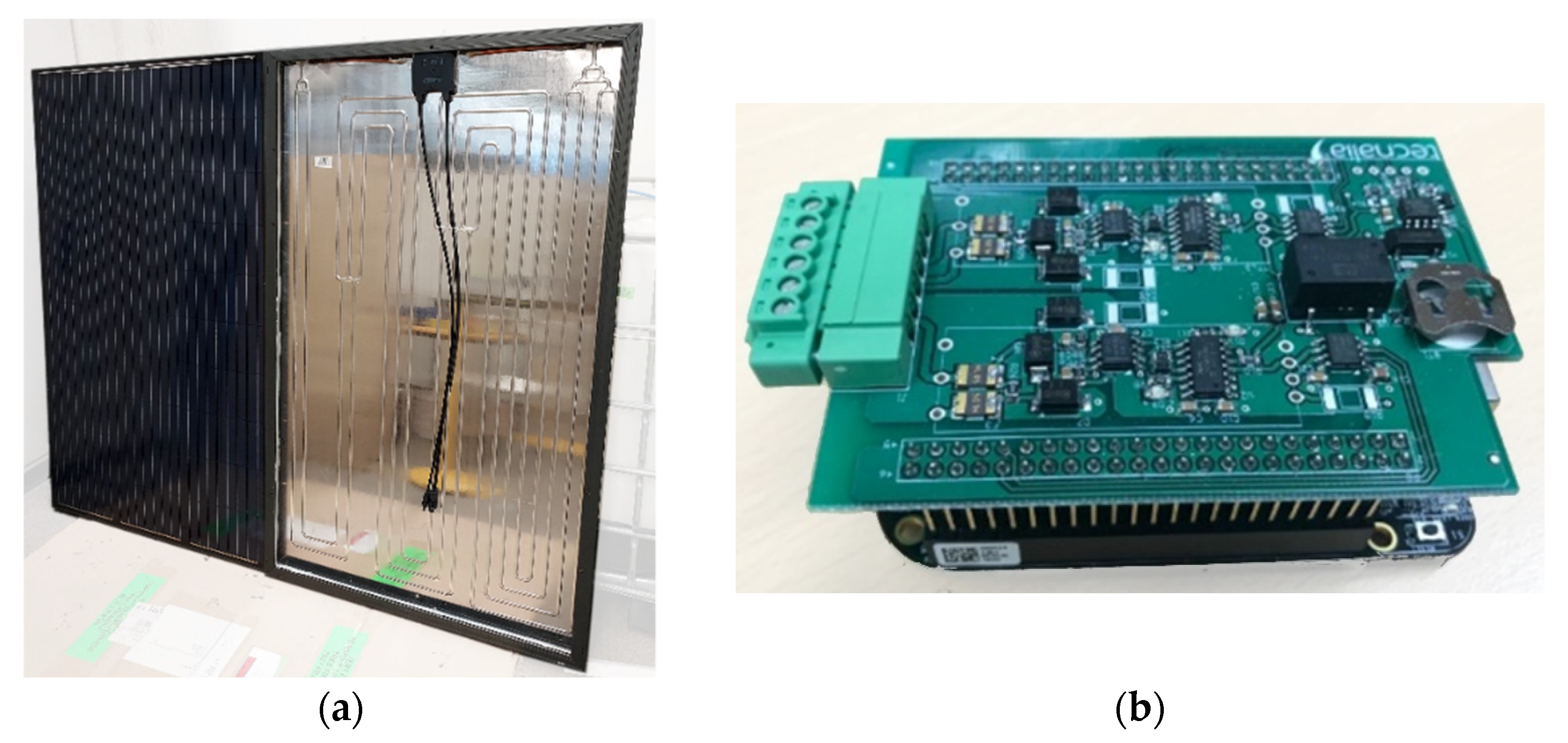
According to these premises, a new PVT collector has been proposed (Figure 2). The collector pretends to be closer to a conventional c-Si PV module in terms of cost, with an additional single residual heat recovery unit. This lightweight solution is manufactured by means of a directly one-step lamination on top of a hard-anodized roll bond thermal absorber, that achieves cost competitiveness while enhancing the heat transfer between PV cells and HP refrigerant. To enable further heat transfer with ambient air [36], the collector has no extra backsheet, thermal insulation or any further mechanical components.

1.2.2. Overall System Control

The solar PVT-based solutions controllers have been traditionally left in a second plane [37,38]. The classical systems hardly require high-powered active elements during operation, where excluding electric back-up systems, the only present loads are the solar field circulation pumps. In such conventional systems, the thermal generation is simply delivered to the tank and the electrical energy is injected into the grid [39]. The recent self-consumption regulation advances are pushing towards more complex system architecture combinations, where PV and ST are combined with HP or other components [9]. These entire solutions must be controlled integrally for ensuring a proper global energy performance, considering not only the thermal but also the electrical generation [40,41,42].

Furthermore, in an nZEB scenario, the local energy generation will not be the only problem to be solved. Thermal and electrical energy supplies will need to be smartly handled to satisfy user needs technically and economically. However, the current solar hybrid solution controllers seem not to be capable of ensuring the required performance [43,44].

Consequently, a new overall system control is presented (Figure 2). The innovative control strategy considers a day ahead DHW consumption prediction routine integrated into a high-level control layer that maximizes the HP operation with just solar resources. Thus, higher solar fractions and self-consumption figures could be achieved, optimizing the overall system performance without affecting end-user comfort or grid impact.

2. Materials and Methods

In order to prove the previously exposed potential benefits, a prototype of the proposed solution was developed, installed and operated for one entire year in a real-use application. The objective of the test is double. First, to experimentally determine the technical performance of the whole solution by means of accurate monitoring. Second, to validate the robustness of the system under extreme working conditions.

2.1. Experimental Set-Up

2.1.1. Real-Use DHW Application

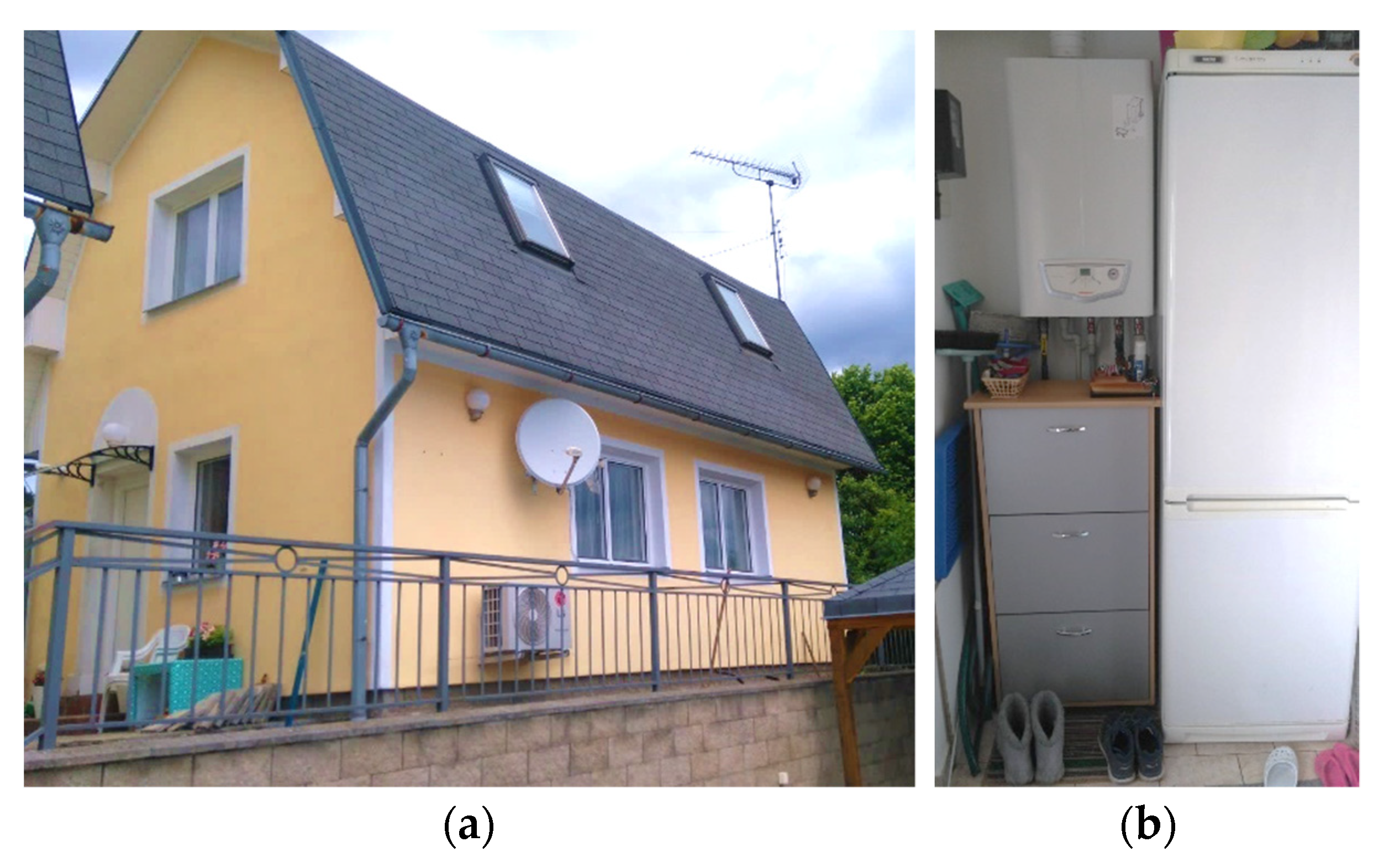
The demonstrator baseline is a single-family house located at Jablonec nad Nisou, Czech Republic (Figure 3). The new solution has been installed to fully supply hot tap water for a 3-member family, replacing the previously existing gas boiler. However, the boiler has not been removed during the test period as it still covers space heating energy needs and may be punctually used as a back-up system, if needed, during the heavy winter season.

As part of a preintervention study, the building usage patterns have been analyzed according to user questionaries. The household accommodates 2 persons during workdays and 4 during weekends. The daily average hot tap water consumption is around 200 L, distributed in early morning showers, short mid-day cooking/washing, and night additional 10 min showers. According to the collected information,

Table 1. Household expected DHW day and month energy demands, according to historical average maximum/minimum ambient and tap water temperatures.

Month	Tamb,max (°C)	Tamb,min (°C)	Ttap water (°C)	QDHW (kWh/Day) *	QDHW (kWh) *
January	0.4	−5.4	4	10.672	331
February	2.7	−4.0	5	10.440	292
March	7.7	−1.0	7	9.976	309
April	13.3	2.6	9	9.512	285
May	18.3	7.1	10	9.280	288
June	21.4	10.5	11	9.048	271
July	23.3	11.9	12	8.816	273
August	23.0	11.7	11	9.048	280
September	19.0	8.7	10	9.280	278
October	13.1	4.3	9	9.512	295
November	6.0	0.2	7	9.976	299
December	2.0	−3.3	4	10.672	330
Year	12.5	3.6	8.3	9.686	3534

* Calculated at 50 °C.

shows the estimated energy requirements to be satisfied.

2.1.2. System and Components Sizing

The DHW application that has been chosen for validation purposes determines the strategy to be used for system sizing. Thus, according to the expected DHW day demand and its consumption profile, the thermodynamic bloc comprising the HP and the thermal energy store (TES) is selected. Traditionally, for DX-saHP, the key parameter to look at at this point is the time interval needed to ensure the entire tank water is heated at the set point. Usually, a maximum time is established. Then the HP and TES are selected to guarantee that in the worst-case scenario the elapsed time needed to reach the setpoint is below the defined one. For the current case study, at the coldest, lower solar resource and higher DHW demand months of January and December, with a 2.5 kW of heat output HP and a 200 L TES the elapsed period is 1.65 h.

However, the new solution to be tested pretends to run mainly on solar resources. For this reason, an inverter HP has been selected. Even at its maximum regime, an output of 2.5 kW of heat would be reached, it will regularly work at lower operation points. Thus, a slightly higher TES volume has been selected. The final volume is 300 L, increasing by 50% the TES capacity and enabling us to heat it up during solar resource availability periods. Thus, the risk of reaching premature HP stops due to the maximum TES temperature being reduced.

Finally, for the selected thermodynamic block, the collection field is sized according to the required cold power for the HP in the previously commented winter period worst-case scenario. For the current case study, with a conventional DX-saHP system, a total of 2.72 m² (2 units of 1.36 m²) of black painted roll bond solar thermodynamic collectors would be enough. However, the new solution is based on PVT collectors and the front layer might have a lower heat transfer capacity. Thus, the selected collection area is increased up to 4.8 m² (3 units of 1.6 m²). Even though 2 units might be enough to thermally run the HP, the additional collector is supposed to add a plus for the critical winter season. To avoid undesired excessive summer HP suction temperatures, independent blocking valves are added to each one of the collectors. An additional PV module is also added in order to enable a comparison of electrical yields.

The prototype key components’ main features are summarized in

Table 2. PVT collector and PV module main features.

Features	Value
Maximum peak power	250 W
Maximum power point voltage	29.53 V
Maximum power point current	8.45 A
Open circuit voltage	37.60 V
Short circuit current	8.91 A
Cell Normal Operating Temperature	45.0 ± 2 °C *1
Short circuit current temperature coefficient	0.04%/°C
Open circuit voltage temperature coefficient	−0.32%/°C
Maximum power temperature coefficient	−0.43%/°C
Operating temperature range	−40 … +85 °C
Backsheet collection area	1.63 m2 *2
Maximum working pressure	10 bar *2
Refrigeration input/output connectors	SAE 1/4′′/3/8′′ *2
Dimensions (length × width × height)	1645 × 990 × 40 mm
Weight (PVT/PV)	30/26 kg

*¹ Valid only for PV. *² Valid only for PVT.

for the PVT collector and PV module, and in

Table 3. HP and TES main features.

Features	Value
Heat output	340 … 2500 W
Electric consumption	240 … 580 W
Compressor	DJ75F0F-20UB
Inverter	PSD101021A
Expansion valve	E2V09USF10
Coefficient of performance	1.4 … 4.3
Auxiliar heating resistance	na
Refrigerant	R134A
Volume	300 l
Maximum working temperature	60 °C *1
Operating temperature range	−5 … +42 °C
Dimensions (length × width × height)	2008 × 550 × 601 mm *2
Maximum working pressure	6 bar
Heat mean transfer	0.025 W/m·K
Material	Stainless steel
Isolation	Injected polyurethane

*¹ For HP operation mode. *² Including HP.

for the thermodynamic block comprising HP and TES.

2.1.3. System Installation

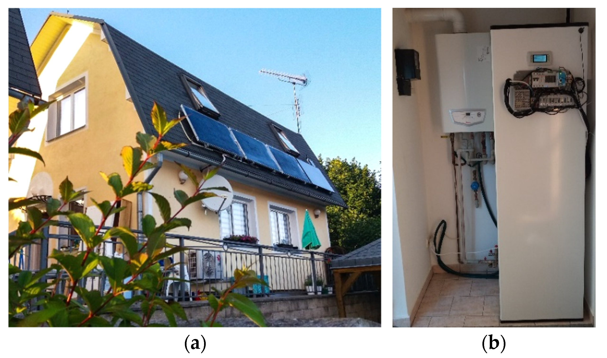
The selected system has been successfully installed in the household (Figure 4). The outdoor unit comprising the solar field has been installed in the same rooftop plane, almost south orientation (−13°) but in a high tilting configuration (70°). In terms of solar resources, the selected plane compared to the optimal (37° slope and 0° south) reduces the annual irradiation by 12.6% but still offers an acceptable winter performance with a 6.3% decrease (for December). Apart from the non-optimal collection plane, there is not any additional significant mismatching in the horizon profile that may affect the energy collection.

The solar field composed is of 3 PVT collectors and the additional PV modules (displayed on the east side) have been installed with identical fixing solutions, so no potential heterogeneity is introduced. In order to measure the potential gap in electrical performance, independent maximum powers for tracking have been deployed for each one of the collectors and modules, based on 2 units of the dual input microinverter APS YC500i.

The refrigerant circuit from the HP to the collectors has an initial common segment of 7 m in length, which is later divided into 3 identical parallel sections of 2 m reaching the collectors, so the different circuits are compensated. Blocking valves have also been included to enable a potential manual disconnection of each one of the collector’s thermal outputs. The return of the circuit is performed in the same way but without any compensation. All the refrigerant pipes are thermally isolated with a 1cm polyethylene.

The indoor unit has been adapted to the available room constraints. Thus, the TES is placed close to the existing gas boiler, so the tank pipes are directly connected to the household DHW circuit.

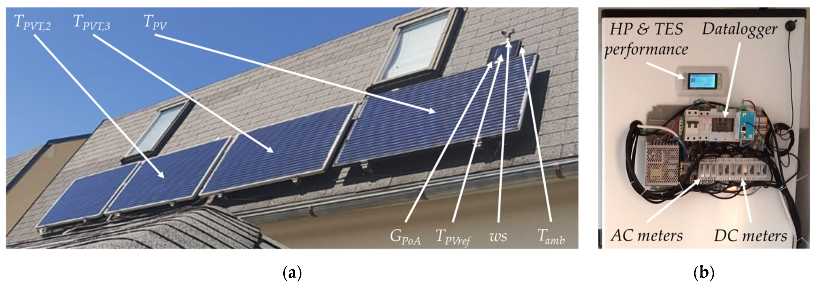
2.1.4. Instrumentation and Data Acquisition

The experimental activity requires accurate monitoring of energy fluxes and further relevant boundary variables to determine the technical performance of both system components and the complete solution. Thus, different kinds of sensors are displayed along the prototype (Figure 5). The most significant variables to measure meteorological conditions, energy collection (solar field), conversion (power electronics for PV and) HP and store (hot water tank) are summarized in

Table 4. A selection of the most significant monitored variables, including the instrument used for the measurement and some additional relevant information.

Instrument	Units	Description	Symbol	Range and Units	Accuracy
MET calibrated cell (Atersa)	2	Global plane of array irradiance	GPoA	0 … 1400 W/m2	±2.2%
	1	Ambient temperature	Tamb	−20 … 100 °C	±0.8 °C
	1	Wind speed	ws	2 … 140 km/h	±3% *1
	1	Crystalline silicon PV module reference temperature	TPVref	−20 … 100 °C	±0.8 °C
RTF-100-S4B-5.0-C8 PT100 (Labfacility)	3 2 at collectors and 1 at module	Middle absorber/backsheet temperature	TPVT,2 TPVT,3 TPV	−50 … 150 °C	±1%
VMU-E DC energy meter (Carlo Gavazzi)	4 one per collector	Voltage	VPVT/PVm,X	0 … 400 V	±0.5% *2
		Current	IPVT/PVm,X	0 … 20 A	±0.5% *3
		Power	PPVT/PVm,X *5	0 … 8 kW	±1%
		Energy	EPVT/PVm,X *5	na kWh	±1%
EM110 AC energy meter (Garlo Gavazzi)	3 Grid balance PV generation HP consumption	Energy	EGrid EPVm EHP	na kWh	±1% *4
µPC HP controller (Carel)	1	Compressor voltage	VComp	na V	±1%
		Compressor current	IComp	na A	±1%
		Evaporation temperature	TEva	−50 … 100 °C	±1 °C
		Suction temperature	TSuc	−50 … 100 °C	±1 °C
		Discharge temperature	TDis	−50 … 100 °C	±1 °C
		Condensation temperature	TCon	−50 … 100 °C	±1 °C
		TES load temperature	TTES,load	−50 … 100 °C	±1 °C
		TES middle temperature	TTES,mid	−50 … 100 °C	±1 °C
		Condenser outlet temperature	TCOut	−50 … 100 °C	±1 °C

*¹ The accuracy for wind speed is valid for 15 … 140 km/h range, but always greater than ± 1 km/h. *² The accuracy for DC voltage is valid for 10 … 400 V range. *³ The accuracy for DC current is valid for 0.05 … 20 A range. *⁴ The accuracy for AC energy is 1.5% for a range of 0.25 … 0.5 A, according to EN50470-3. *⁵ The term E_PV is left for the total solar field electrical output.

.

The selected monitoring architecture is based on in-site measurements that are immediately transduced into Modbus over RS-485 by the sensors themselves. Then the data is remotely requested and handled by a datalogger service in the same Beagle Bone board where the control is implemented. The 69-variable monitoring register is gathered every minute and stored on a daily basis in csv files. The control and data logging board have an internet connection by means of a router with a VPN. A remote copy of local content is created weekly.

2.2. Data Analysis, Cleaning and Processing

The applied methodology is essentially based on the analysis of experimental data. The monitoring activity provided dataset is postprocessed to enable a better interpretation and further discussion.

The gathered system performance is first analyzed in detail. The day-based files have an automatic checking algorithm. The procedure only enables us to filter entire day performance days with all dataset variables in range. Furthermore, all days are carefully manually analyzed using specific timeseries templates to filter any additional errors. Thus, days with partial operation, monitored variable outlyers or additional reported phenomena are removed at this stage. Any kind of gap filling is not considered.

The analysis continues only with the valid-day dataset. For this selection, several intraday parameters and day-aggregated energy values are calculated. Additionally, day representative key performance indicators (KPI) are obtained.

Finally, day representative KPIs are once more aggregated in a monthly-based approach. For this analysis, the average, median or accumulated values of day-based KPIs are considered for monthly-based periods.

2.3. Key Performance Indicators

The determination of these KPIs is performed according to the common agreed procedure established within different Tasks of the International Energy Agency Solar Heating and Cooling programme [45].

2.3.1. System Level

A set of four main KPIs has been considered to characterize system operation. The renewable energy share represents the local non-fossil fuel potential:

$$RES={\displaystyle \int }\frac{{\dot{Q}}_{HP}}{P_{Grid, NC}}$$

(1)

where $Q_{HP}$ is the HP heat output, which for the current DX-saHP solution is not directly measured but calculated based on the compressor manufacturer data and monitored T_Eva, T_Con and HP controller compressor frequency.

The self-sufficiency ratio shows the real solar field output potential to cover the HP electric consumption needs:

$$SSR={\displaystyle \int }\frac{P_{PV}}{P_{HP}}$$

(2)

where $P_{PV}$ is the aggregated electric output of the three PVT collectors and the corresponding one for the PV module. $P_{HP}$ is the HP consumption, which considers the compressor but also additional devices.

The self-consumption ratio to determine the real PV output potential to cover the HP electric consumption needs:

$$SCR={\displaystyle \int }\frac{\min (P_{PV},P_{Grid)}}{P_{PV}}$$

(3)

where $P_{Grid}$ is the system grid consumption in the scenario of non-PV production.

Finally, the solar fraction, to obtain the utilization ratio of the solar resource at the energy collection field:

$$SF={\displaystyle \int }\frac{P_{PV}+{\dot{Q}}_{PVT}}{4·A_{PVT/PV}·G_{PoA}}$$

(4)

where $A_{PVT/PV}$ is the aperture area of the PVT collectors or PV module, in this case identical. $Q_{PVT}$ is the PVT collector field heat output, which, as in the case of $Q_{HP},$ could not be locally measured and has been obtained as a function of monitored T_Eva, T_Con, HP frequency and manufacturer tests data. The ambient gain for PVT collectors due to below ambient operation is included in this calculation procedure and should be removed for genuine SF obtention, but there is still no confident procedure to decouple it.

2.3.2. PVT Collectors

The quantification of the performance gap between the PVT collector and the reference PV module is the goal of the following two specific KPIs that are proposed. One of them is focusing on the potential performance ratio increase:

$$\Delta P{R}_{PV}^{PVT}=\frac{\frac{{{\displaystyle \sum }}_{i=1}^3\left(P{R}_{PV{T}_i}\right)}{3}-P{R}_{PV}}{P{R}_{PV}}$$

(5)

where $P{R}_{PV{T}_i}$ is calculated for each one of the collectors as follows:

$$P{R}_{PV{T}_i}={\displaystyle \int }\frac{P_{PV{T}_i}·f_{PV}^{PV{T}_i}}{A_{PVT/PV}·G_{PoA}}$$

(6)

with $f_{PV}^{PV{T}_i}$ as the maximum power point deviation correction between each one of the collectors and the PV module used as reference. $P_{PVT}$ is the electrical output of the 3 PVT collector-field. The electrical characteristics of each collector and module have been obtained with an indoor flash tester and in the same way the $P{R}_{PV}$:

$$P{R}_{PV}={\displaystyle \int }\frac{P_{PV}}{A_{PVT/PV}·G_{PoA}}$$

(7)

The second KPI tries to clarify if the PR deviation is correlated with the expected lower operation temperature of the PVT collectors [46]. Thus, the day’s average PVT collector temperature difference with the PV module reference is calculated:

$$\Delta \overline{T}{ }_{PV}^{PVT}={\overline{T}}_{PVT}-{\overline{T}}_{PV}=\frac{{{\displaystyle \sum }}_{i=1}^3\left({\overline{T}}_{PV{T}_i}\right)}{3}-{\overline{T}}_{PV}$$

(8)

where ${\overline{T}}_{PVT/PV}$ is calculated for each one of the collectors and modules as follows:

$${\overline{T}}_{PV{T}_i/PV}=\frac{1}{N}{\displaystyle \sum }_{t=0}^N{T}_{PV{T}_i/{\mathit{PV}}_t}$$

(9)

Additionally, conventional conversion efficiencies are proposed. In the case of the PV module just considering the electric output power:

$${\eta }_{PV}={\displaystyle \int }\frac{P_{PVm}}{A_{PV}·G_{PoA}}$$

(10)

where $P_{PVm}$ is the electrical output of the PV module, and for the PVT collector adding the heat outcome:

$${\eta }_{PVT}={\displaystyle \int }\frac{P_{PVT}·{\dot{Q}}_{PVT}}{A_{PVT}·G_{PoA}}$$

(11)

2.3.3. Heat Pump

The instantaneous operation of the HP is characterized by the coefficient of performance, and analogously over a specified period, the performance factor is used:

$$PF=\frac{Q_{PVT}}{E_{HP}}$$

(12)

which relates to the corresponding integrated quantities of provided heat and consumed electricity $E_{HP}$.

In the same way, the net performance factor of the HP could be obtained, where just the self-consumed energy is considered in the balance:

$$P{F}_{net}=\frac{Q_{PVT}}{E_{HP}-E_{SC}}$$

(13)

2.3.4. Thermal Energy Store

The hot water tank performance is analyzed by means of four temperature KPIs. Three of them are based on middle tank (half-height) temperature, which could be considered as the most representative of the entire water volume. Thus, the minimum value during the period is calculated:

$$T_{TE{S}_{50}{}_{\min }}=\min \left(T_{TE{S}_{50}}{}_t\right)$$

(14)

Additionally, the day average is obtained:

$${\overline{T}}_{TE{S}_{50}}=\frac{1}{N}{\displaystyle \sum }_{t=0}^N{T}_{TE{S}_{50}}{}_t$$

(15)

Finally, the day cycle temperature delta is represented:

$$\Delta T_{TE{S}_{50}}{}_{\min }^{\max }=T_{TE{S}_{50}{}_{\max }}-T_{TE{S}_{50}{}_{\min }}=\max \left(T_{TE{S}_{50}}{}_t\right)-\min \left(T_{TE{S}_{50}}{}_t\right)$$

(16)

The last KPI is based on the upper tank temperature day average value:

$${\overline{T}}_{TE{S}_{100}}=\frac{1}{N}{\displaystyle \sum }_{t=0}^N{T}_{TE{S}_{100}}{}_t$$

(17)

2.3.5. Average Day Energies

Additionally, for the main energy fluxes, the day accumulated values are considered within the KPI analysis: the solar field electrical output ($E_{PVac}$), which includes PVT collectors and PV module outputs at the AC side of the inverter; the PVT collector heat ($Q_{PVT}$); the HP electrical consumption ($E_{HP})$ and provided heat ($Q_{HP}$); and finally, the grid consumption ($E_{GC}$).

3. Results and Discussion

The described system has been operated for one entire year. The obtained results are presented below. Initially, a day-based analysis is carried out. Then, month-aggregated KPIs are discussed. Finally, month-days statistical analysis is presented.

3.1. One Day Performance

3.1.1. Spring/Autumn

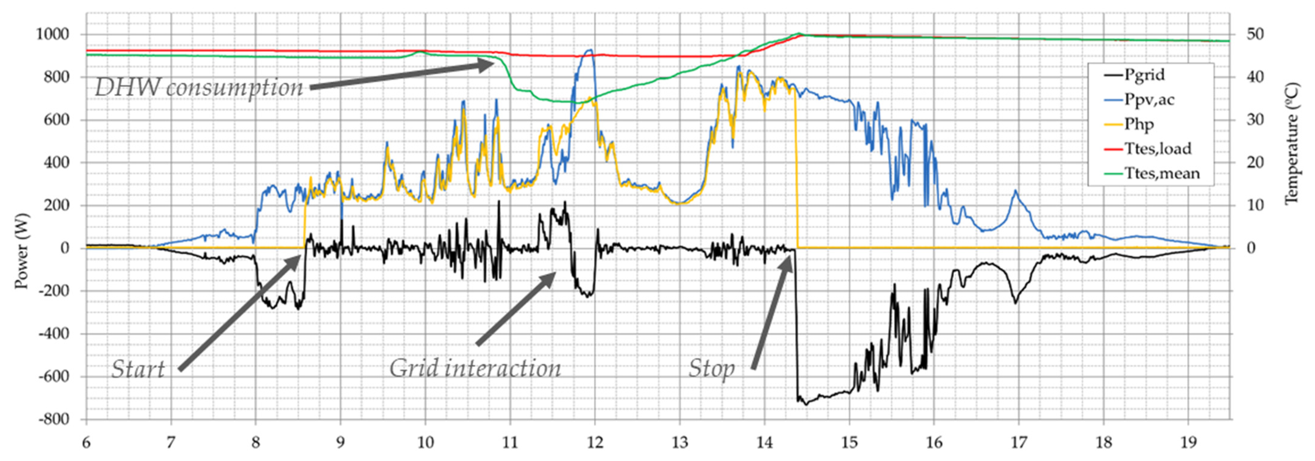
The considered day for the analysis is the 15 April (Figure 6). This spring day has a 4.4 kWh/m² plane irradiation, a 16.3 °C mean ambient temperature and almost no wind (0.54 m/s). The smart controller of the solution starts up the operation at 8h35, with a relatively high TES average temperature of 44.7 °C. The HP is continuously in regulation mode, copying the PV production till 14h22, when it reaches the 50 °C setpoint and stops. In the operation period, the TES mean temperature is reduced to 33.3 °C at 11h45 due to a medium DHW consumption, although the load temperature does not go below 45 °C. In the almost 6-h operation, the HP only reaches its maximum heat output regime for 30 min between 11 h and 12 h, instead, it manages to heat the entire TES without impacting the grid consumption or affecting user comfort.

The system-level KPIs evidence great figures for RES (95.8%) and SSR (142.9%), mainly driven by good solar resources. The non-evening operation reduces the SCR to 63.1%, but still shows a high capability to self-consume almost all the energy of the operating period (apart from the 25 min duration grid consumption at 11h15 and 15 min injection at 11h45). The non-HP operation period and the low regime during operation are responsible for not gathering higher SF (30.5%). A half of SF is for electricity production, which shows that for such a day there is still much more potential heat to be produced.

3.1.2. Summer

The day for the analysis is the 15 July (Figure 7). It is a sunny morning with some clouds appearing in the afternoon, with a total of 5.9 kWh/m² of plane irradiation, 21.8 °C mean ambient temperature and no wind (0.08 m/s). The system presents a first-day operation at 9h02, with a reasonably conservative TES average temperature of 32.9 °C. The HP is working in regulation mode following the PV production setpoint. After 3 h of operation, the TES is completely heated, and in consequence, the HP is stopped. During the evening, a first low DHW consumption event could be noticed at 16h45, but the second one around 21h15 significantly reduces the TES available heat. Thus, when the TES average temperature goes below 20 °C the second operation period starts till almost midnight when a defined minimum TES temperature of 30 °C is reached.

The system-level KPIs show more good RES (91.4%) with the expected high SSR (175.2%). The same pattern non-evening operation reduces the SCR to 38.6%. The narrow summertime HP operation periods and lower thermal loads limit the SF (36.5%). However, the system performance during the operation period at ambient temperatures up to 33 °C validates the system concept also for hot locations.

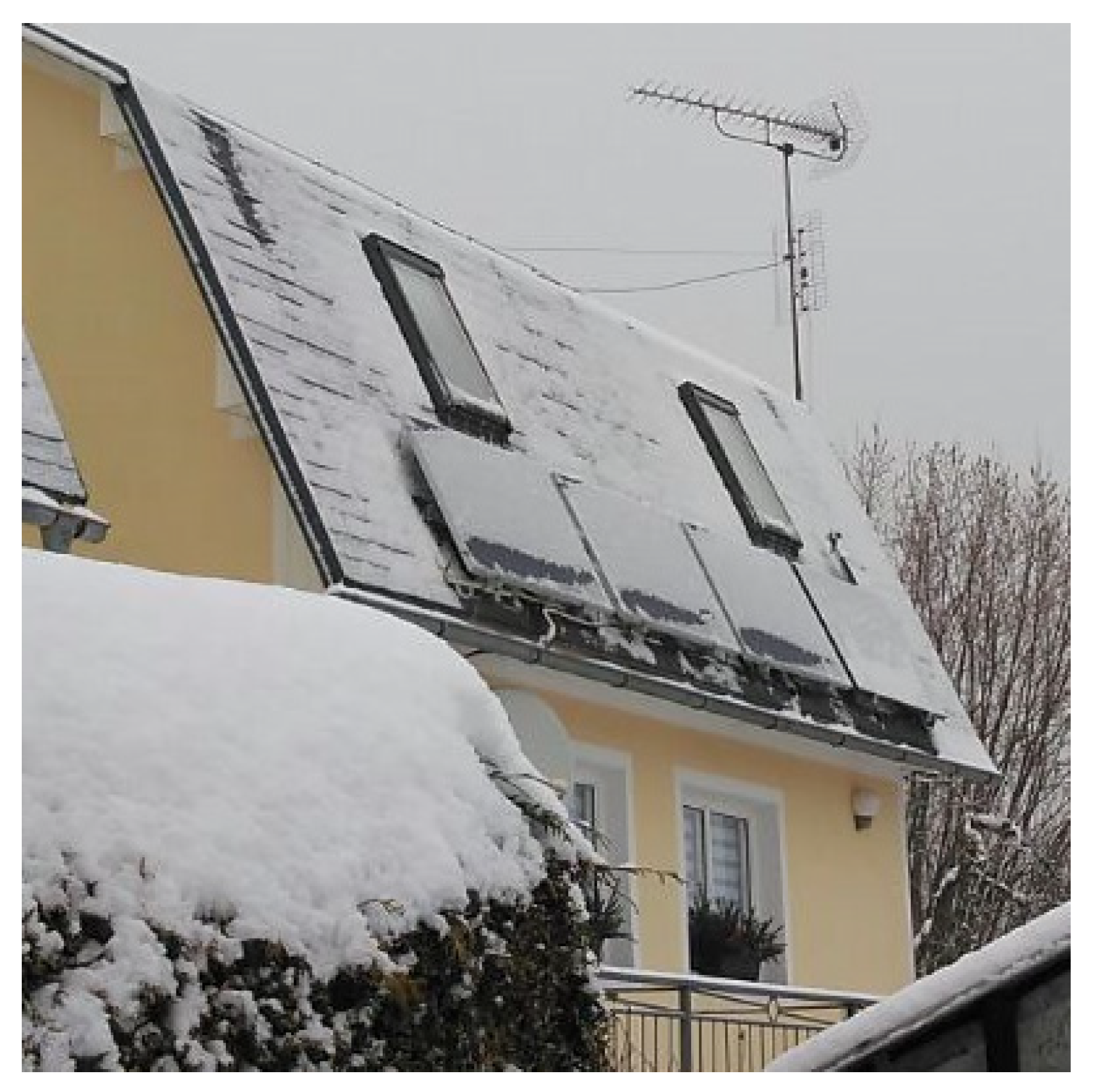
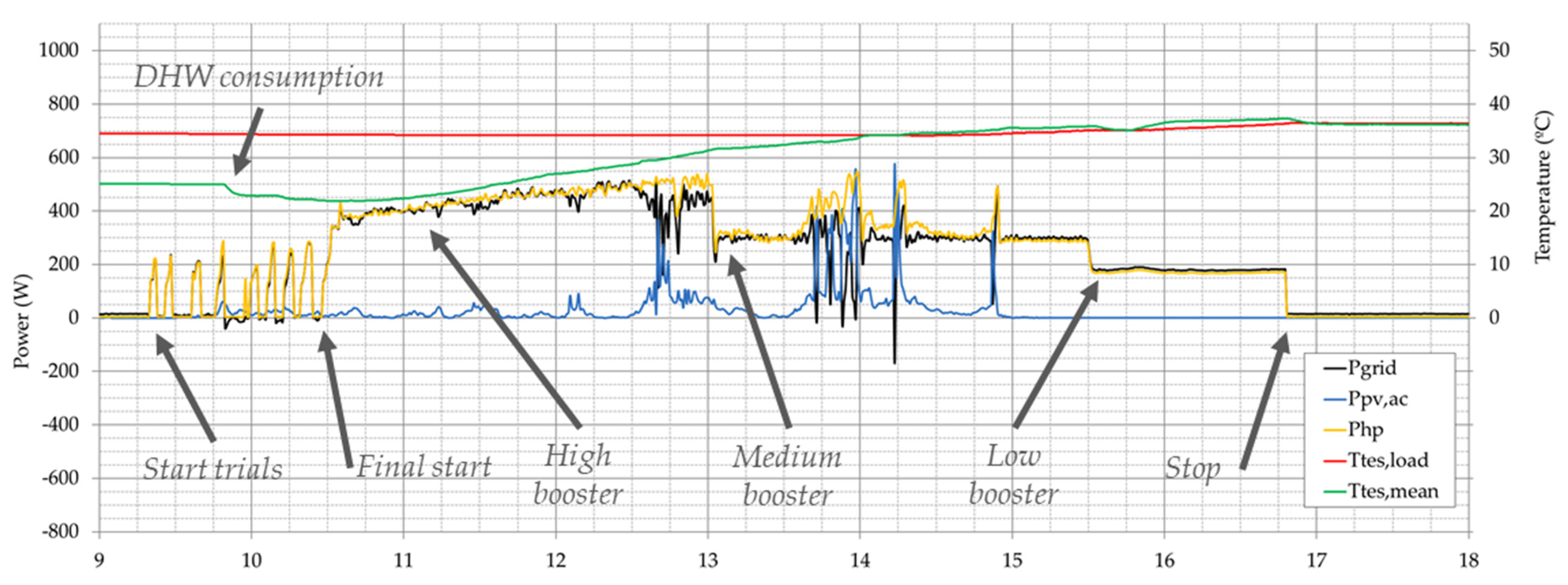
3.1.3. Winter

Winter at the testing site is hard, with common snow precipitation (Figure 8). The operation conditions within this period are characterized by low or null PV production. A representative day of such boundary conditions is the 10th December. The plane of array irradiation is 0.46 kWh/m², 1.3 °C mean ambient temperature and almost no wind (0.43 m/s). Figure 9 shows the day operation profile with up to 8 start attempts from 9h20 onwards. The low ambient temperature (1.3 °C) and iced collectors make the HP difficult to start, but after 1 h of trials, the HP is running with identical ambient temperature conditions. In the absence of PV generation, the 6-h operation profile has an initial period with the HP working at a high-level booster till 13h00, then the booster is reduced to a medium-level till 15h30 and, finally, low-level booster operation is extended till 16h45. Even for these kinds of days, during all-day operation, the HP restores TES to secure levels with a day cycle temperature delta of 15.4 °C.

In this case, the system-level KPIs are lower but still relevant RES (61.9%), mainly driven by HP contribution. The SSR is reaching just 9.4%. On the other side, the low PV production and high HP consumption artificially enhance the SCR up to 98%. The SF does not make sense, as the ambient air contribution is much greater than the solar gain.

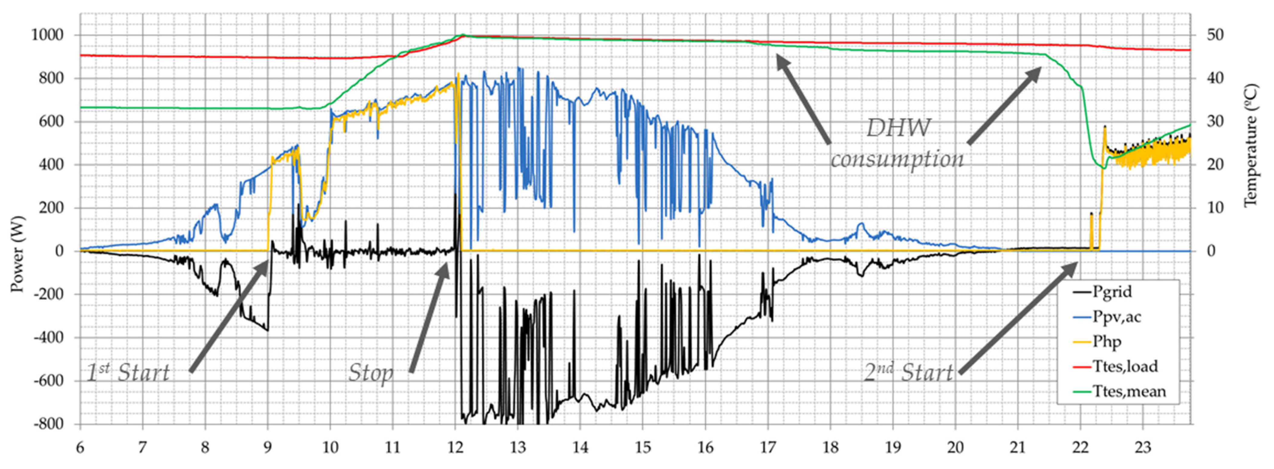
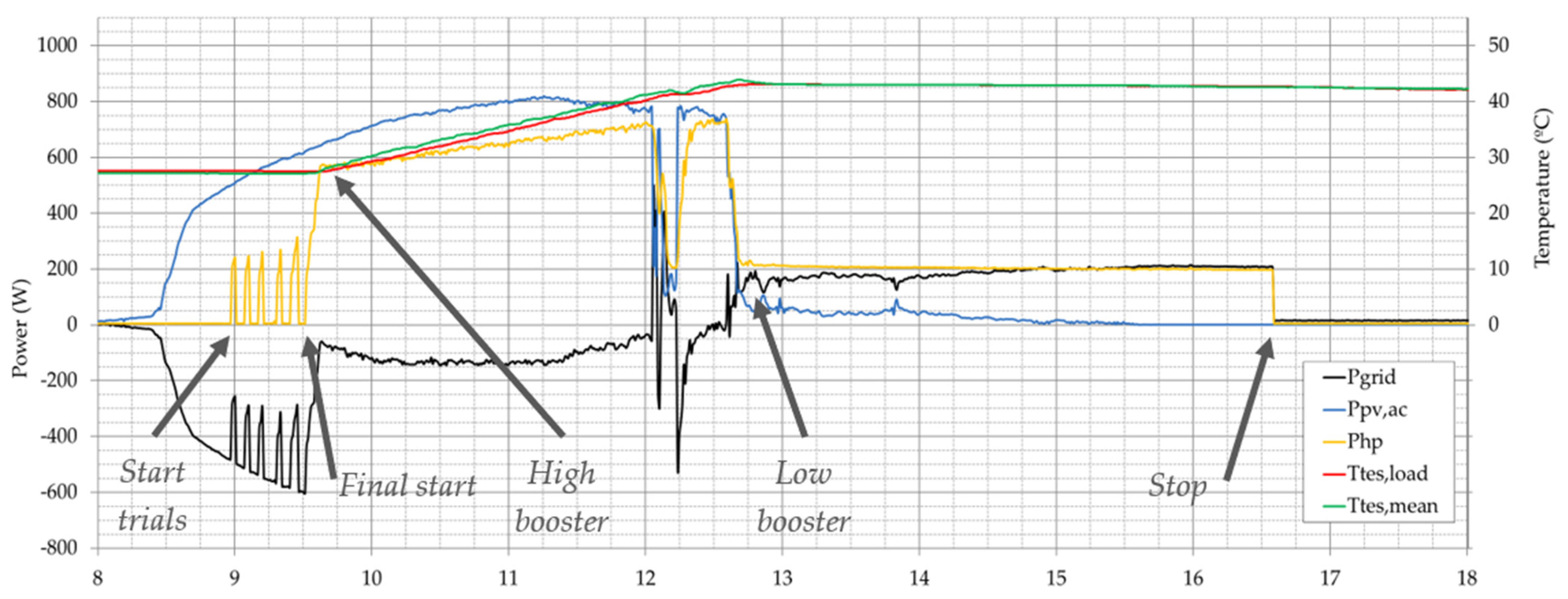
The previously presented day is the most common day type in the period and that is its underlying value. However, the low solar contribution may reduce the interest of its analysis, as it could be considered a simple air-water HP. Thus, an exceptional high irradiance cold day is discussed below, the 14th January. The plane of array irradiation is 3.03 kWh/m², −2 °C mean ambient temperature and once again no wind at all (0.46 m/s). The day is a Sunday, and the family seems to be not at home, as there is no DHW consumption. Figure 10 shows the day operation with a repetitive accidental starting pattern. The system finally starts running at the 6th attempt around 9h30. The high irradiance morning drives the HP under the highest operation range till 12h40, even with an excess electricity grid injection. The morning period is only affected by a short 20 min cloud, but the great solar contribution suddenly disappears. The afternoon is characterized by almost null irradiation (5% of the day), but the system continues running at low-level extended booster till 16h50. The 7h day operation increases the TES temperature to 15 °C.

The system-level KPIs are turning around compared to the previous low irradiance winter day. The RES increases to 86.9%, boosted by the morning period operation. In the same way, SSR is also improved to a value of 76%, but it is significantly reduced due to non-effective long afternoon operation. The reached SCR is high (73%), based mainly on the morning good control strategy. The SF is 40.9%, limited by HP cooling capacity during the high solar resource morning period.

3.2. Considered Versus Real Boundary Conditions

The expected boundary conditions are hardly close to real ones. The comparison of wide testing periods usually concludes with significant deviations that may impact the results. In the current experimental campaign, two main comparisons have been carried out.

On the one hand, the deviation between the previously expected DHW consumption and the final observed one. Usually, this initial DHW demand is the main parameter driving the sizing and the savings calculations. The comparison contextualizes the one-year performance, but these initial calculations are not further used in the analysis. The DHW energy consumption reference is obtained according to the end-user reported information by means of questionnaires and some additional calculations, basically the location boundary conditions tap water temperature. The entire year experimental dataset initial analysis shows a huge deviation between the expected and the final values (Figure 11). There are several reasons underlying the deviation:

• The daily hot tap water volume estimations based on previous interviews were oversized for all the testing period;
• The occupation of the household has faced several absence periods, mainly during summertime and during the month of February;
• An error and reparation in the HP, resulting in 14 days off during November;
• The tap-water temperature used for demands calculation has been lower than the real one for all the testing period;
• For the period starting in November till March, excepting February for the previous remarks, the experimented lower demand is more impacted by system control strategy than lower real demand. Evidence of this phenomenon is the lower monthly average daily mean TES₅₀ temperature.

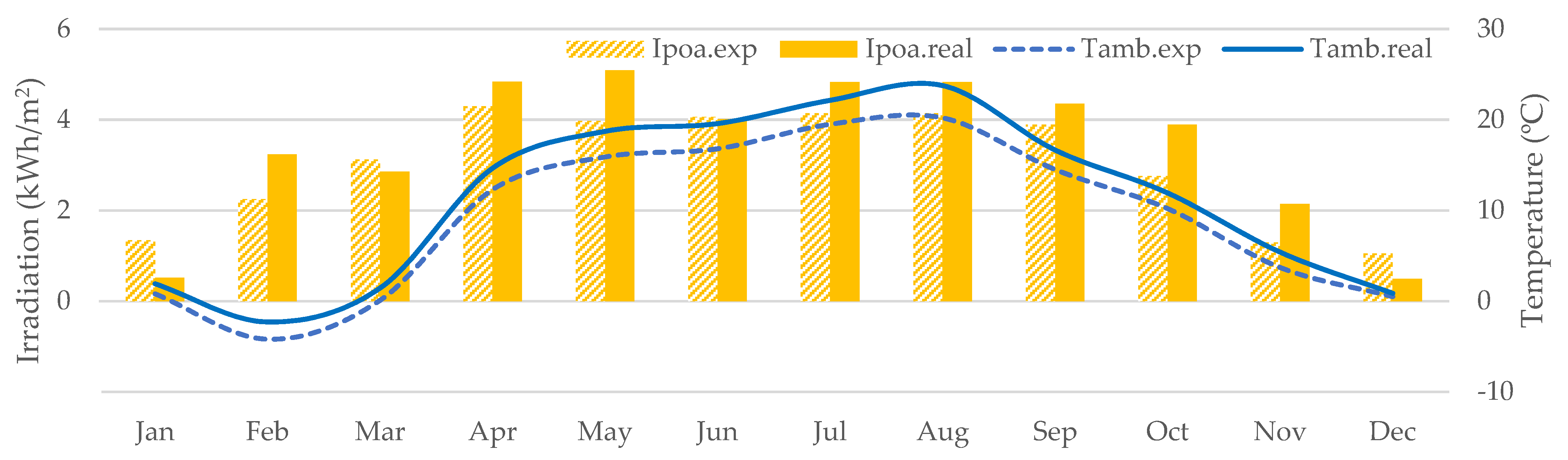
On the other hand, the solar resource has been checked. The values used as a reference are the PVGIS Sarah2 database [47] ones for one decade. For irradiation, the annual measurement is 13.1% above while the temperature is 2.04 °C higher (Figure 12). The typical meteorological year deviations are common, the local irradiance measurements have been additionally checked with specific test-period satellite data, showing a final deviation of −2.8%. For PV output the tool shows a higher yield, aligned with the initial irradiation deviation, but with a clear different pattern for the months of January and December due to not proper snow consideration.

3.3. Average Day Energy Analysis

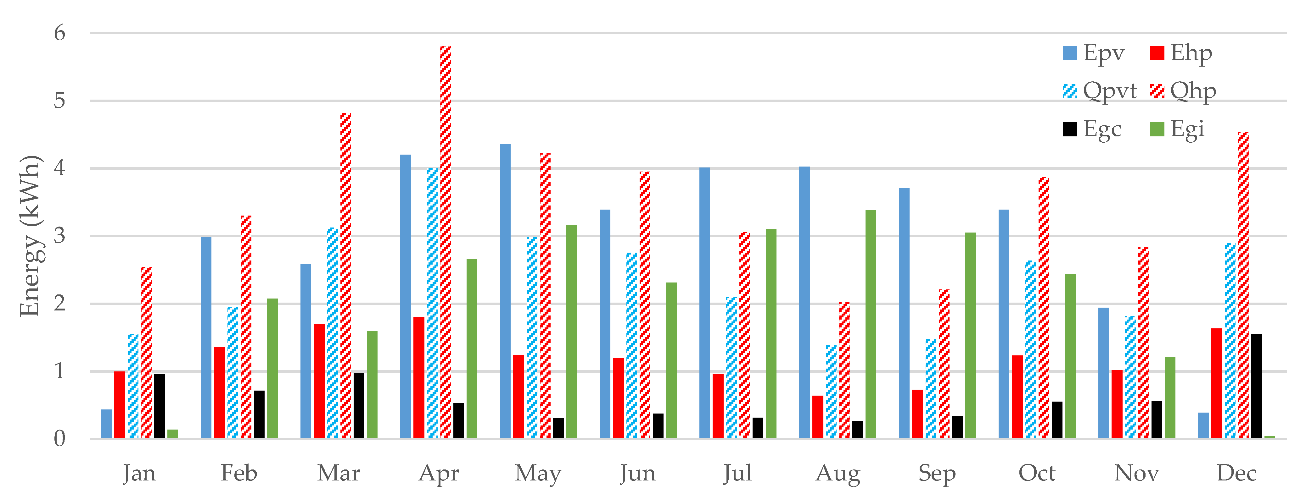
The monthly average daily mean energy magnitudes are illustrated in Figure 13. As commented before, the electric output of the solar field performs as expected, with a high mismatch between winter and summer. The real DHW energy need determines the required heat to be delivered and in consequence HP output. According to controller strategies and meteorological boundary conditions, the HP electric consumption and PVT field provided heat are determined, with respective maximum average day values of 1.8 and 4 kWh reached in April. Finally, the grid energy consumption shows a reasonable profile with imported energy below 1 kWh for all the periods except for December.

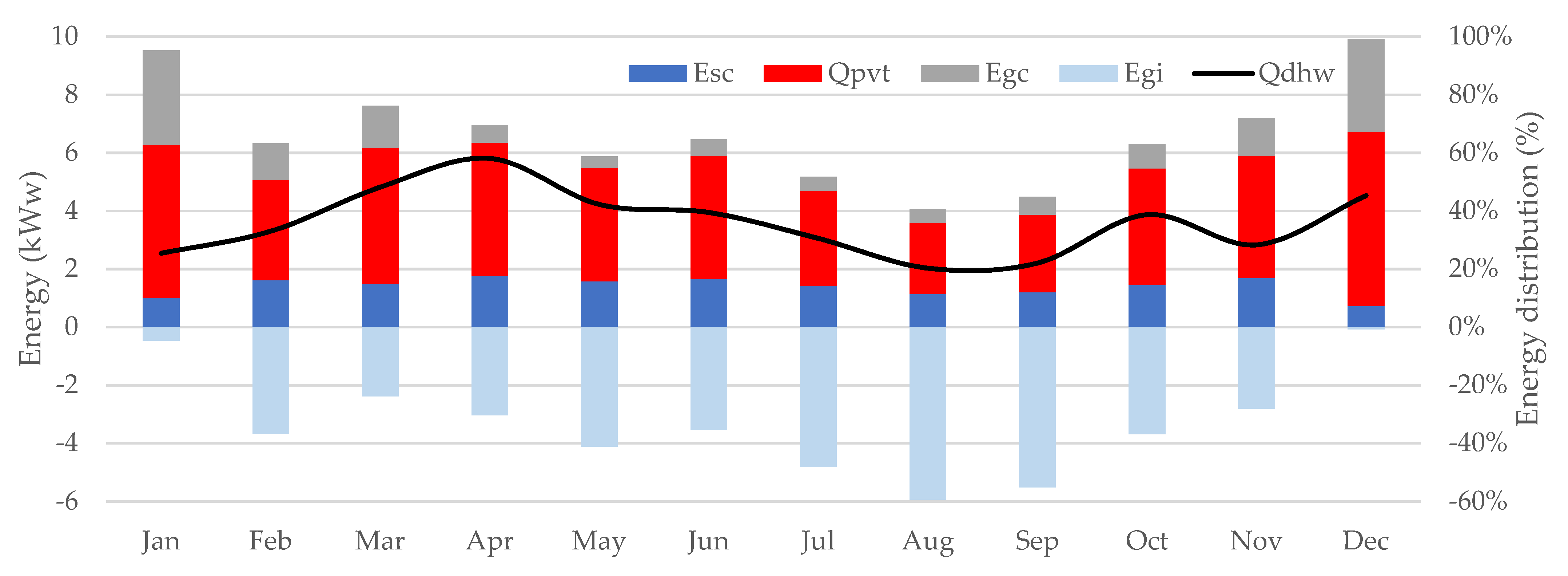
The contribution of each one of the main energy terms to the whole DHW demand is shown in Figure 14. Between 61 and 71% of the final energy is delivered by the PVT field in heat mode. The solar field electrical self-consumed output contribution is in the range of 7.8 to 32%. The last contributor is the grid, with a variable supply of 7.4 to 38%.

The entire year aggregated energy by type is listed below:

• $E_{PVac}$ = 1050 kWh;
• $Q_{PVT}$ = 855 kWh;
• $E_{HP}$ = 431 kWh;
• $Q_{HP}$ = 1287 kWh;
• $E_{GC}$ = 220 kWh;

3.4. Monthly Average Daily KPI Analysis

3.4.1. System Level

The four main KPIs selected to characterize entire system performance are displayed in Figure 15 for the average day values. The RES is above 60% for the whole period, reaching its maximum of 92% for the month of May. The SSR shows the expected greater variability, with a maximum in August (470%) and a minimum in December (18%), affected mainly by the annual fully decoupled DHW energy demand and solar resource. On the opposite side, the obtained SCR is maximum for the winter period (94% for December) while is reduced to 17% for the month of August. The higher values are linked to low irradiance and long HP operation days. Finally, the SF is in the range of 22–159% for August and December, respectively. Days with almost no irradiation but high PVT thermal output, due to wind and infrared energy collection, leading to above 300% values are saturated.

For the entire year’s performance, the obtained system-level average day KPI results are 83% for RES, 220% for SSR, 41% for SCR and 46% for SF. The same KPIs obtained for integration of the entire year are 86%, 204%, 28.5% and 25.7%. The previously commented day and month-based results are reduced for the entire period analysis, especially for SCR and SF. The reason is that the high energy resource summer days with short HP operation are too weighted in this annual analysis. The high RES is basically based on HP performance and enhanced by solar field contribution. The obtained SCR shows good underlying control performance. The obtained SSR and SF results are huge, but somehow artificially boosted due to summer season high solar resource weight and DX-saHP ambient heat collection, respectively.

3.4.2. PVT Collector Versus PV Module

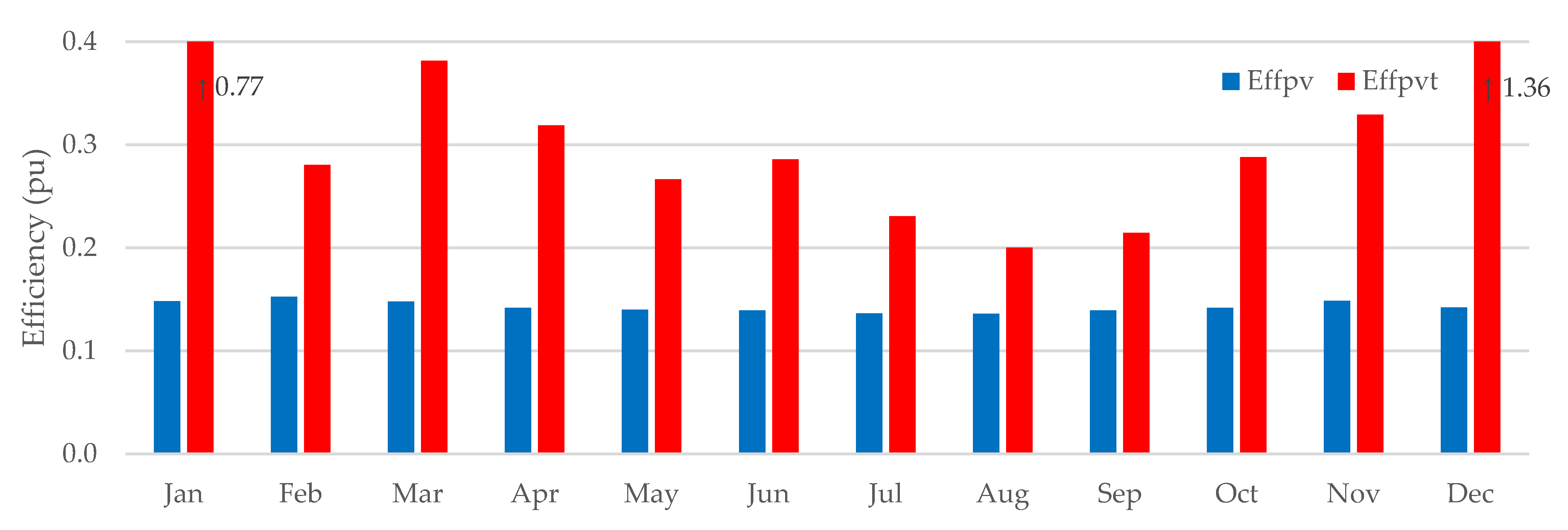
The conversion efficiency of PVT collectors is higher than the same size and identical PV technology modules [30] due to the additional thermal output. However, the final energy performance usually depends on the application or the PVT operation mean temperature and on the classical efficiency versus heat quality dilemma. The period conversion efficiencies determined for the testing period are shown in Figure 16. Apart from the coldest month peaks, due to low resource and ambient energy collection, the rest of the winter months show higher PVT values with a significantly greater thermal side contribution. However, for the high irradiation and hot month of August, the PV influence on efficiency is larger than the electrical one. In annual terms, the PV converts 13.9% of incident solar energy, while PVT reaches 37%.

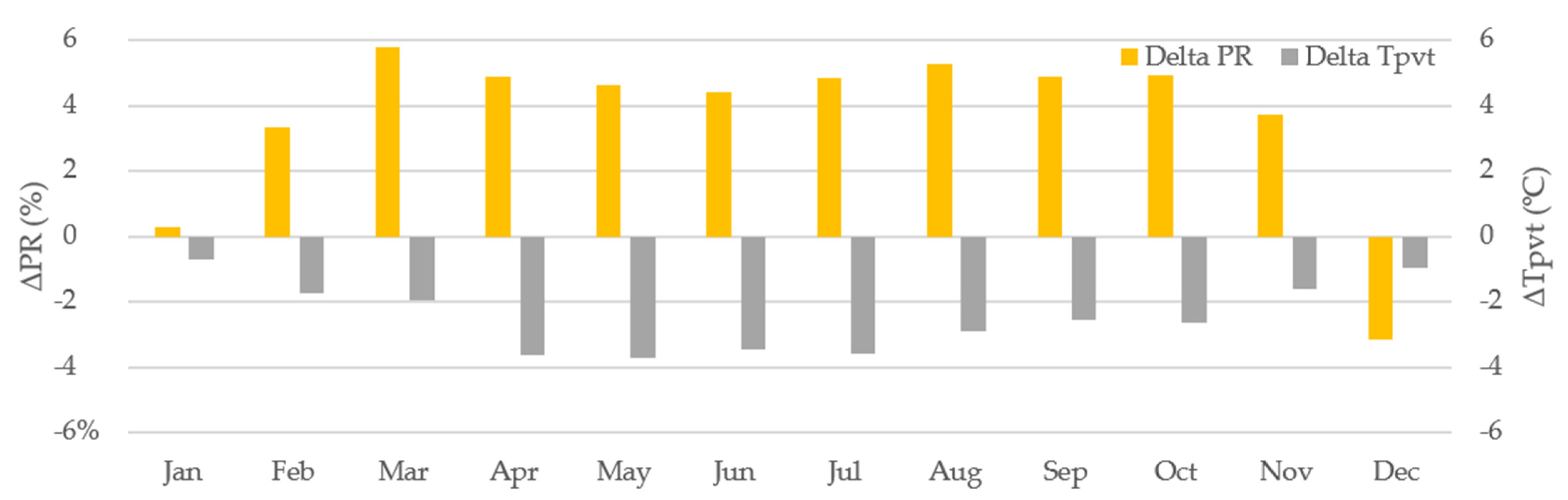
Additionally, in the dually driven DX-saHP tested solution, the PVT collector is not required to operate at high temperatures to offer valuable heat and as a result, the electrical output is not reduced. Figure 17 evidences that the PVT extracted heat reduces from almost 1 to 3.7 °C the average temperature of the PVT collector absorber versus PV module backsheet. Due to the cooling, the electrical PR of the PVT collector is improved for almost all the months, except January and December, affected by heavy collector front layer condensation and icing. However, according to datasheet values, the temperature reduction of 1 K should be traduced in a 0.43% increase in the PR, but the obtained PR results are not in consonance, which might suggest an optimum cooling during high irradiation periods. Finally, the year base result concludes with a PR increase of 4.5%, achieved not only by the HP active cooling but also by better natural convection.

3.4.3. Heat Pump

The KPI selected to determine the HP operation is the PF, the conventional and the boosted. Figure 18 shows the PF oscillation between 2.3 and 3.4, in accordance with datasheet ranges. However, when the net grid imported energy is considered the PF is significantly improved. Even for the winter solstice, the obtained values are similar, during the summer period it reaches median values between 20 and 30. For the calculations, singular values with null grid consumption are not considered.

3.4.4. Thermal Energy Store

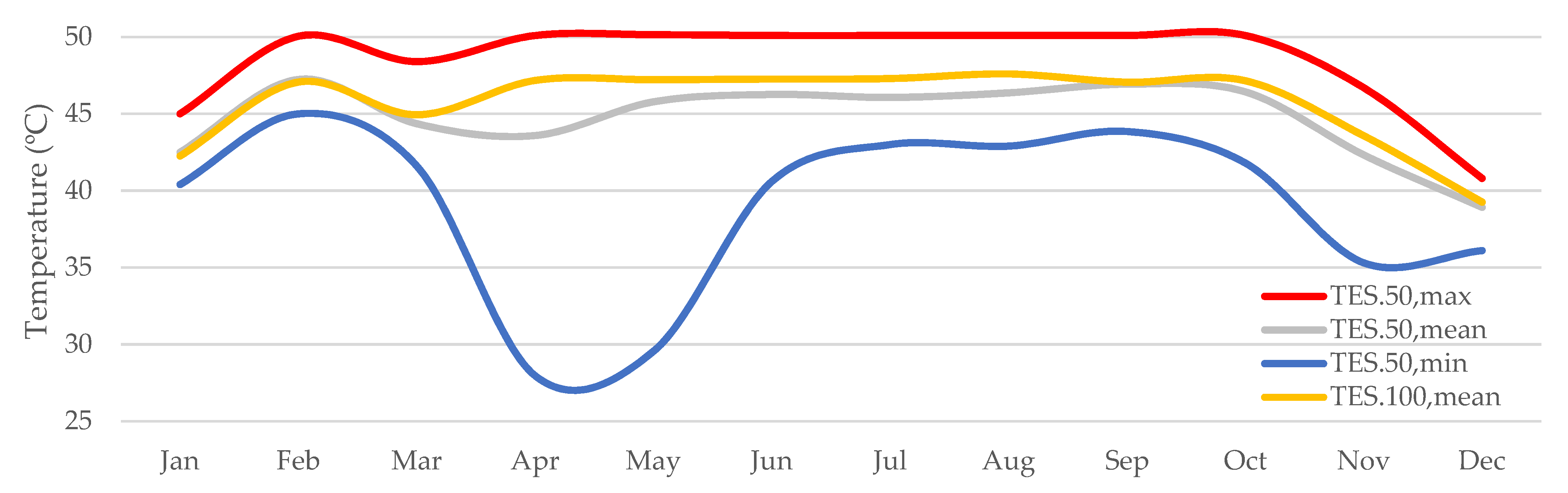
The TES operation key temperature evolution indicates the end-user comfort over the testing period. Figure 19 illustrates the TES KPIs. The tank water volume is the representative temperature range $\Delta T_{TE{S}_{50}}$ during almost all the period is below 8 K. However, for some months the minimum day average temperature is reduced beyond desirable values, mainly driven by laxer controller parameterization (April–May), although no critical points are reached. The November–January period evidences the already previously commented lower TES state of charge, with the minimum for December. For this scenario, the average DHW load temperature is 39.3 °C.

The end-user gathered experience after the experimentation period concludes comfort levels have overall been achieved in terms of DHW service temperature even in hard winter times. Only a couple of days with punctual low TES temperature information shown at HP display have been reported, mainly during the beginning of the testing period. However, the gas boiler that was left as a potential backup has not been connected.

4. Conclusions

Global energy consumption is estimated to be increased over future decades, up to 50% by 2050. At the same time, it is imperative to reduce greenhouse gas emissions by 45% by 2030, compared to 2010 levels, while reaching net zero emissions by 2050. The last COP26 emphasized the urgency and opportunities of moving to a carbon-neutral economy. In the meantime, EU building stock is responsible for 40% of the energy consumption and 36% of CO₂ emissions. However, in the current energy crisis scenario, the European Commission seems to have a clear roadmap toward energy sector decarbonization.

Most of those buildings to be decarbonized need to meet electricity and heat demands. In the nZEB scenario, most of the consumed energy would need to be generated locally by means of renewable solutions that nowadays seem not to provide an attractive performance or cost-competitiveness. Solar-based technologies tend to be the most promising ones, but for highly densely populated and restricted areas, the usual PV or ST single approaches may not be efficient enough.

The current work is focused on the experimental analysis of the dual use of the solar resource by means of hybrid PVT collectors and their smart combination with direct expansion HPs through predictive control strategies. For that purpose, a solution with several innovations in the collector and in the overall control strategy was developed. A real-use single-family house has been selected for hosting the test at a continental climate (Jablonec nad Nisou, Czeck Republic) for a DHW application over one-year of operation. The sizing of the system has been carried out. The system comprising three PVT collectors and one PV module, dually connected to an inverter DX-saHP with an oversized TES and a predictive control has been properly installed, commissioned and fully accurately monitored. The recorded dataset has been postprocessed according to specific internationally recognized procedures for PVT plus HP systems.

After one entire year of the experimental campaign the obtained system-level average day KPIs show 83% for RES, 220% for SSR, 41% for SCR and 46% for SF. For the entire period of aggregation, the KPIs are 86% for RES, 204% for SSR, 28.5% for SCR and 25.7% for SF, due to the impact of common summertime high energy resource short HP operation days. The high RES is essentially based on HP performance and enhanced by solar field contribution. The obtained SCR shows good underlying control performance. The obtained SSR and SF results are huge, but somehow artificially boosted due to the summer season’s high solar resource and DX-saHP ambient heat collection. The overall good performance results are endorsed with monthly level analyses, which show the DHW demand is well covered even for the most critical months. For day-based analysis, a detailed intraday performance has been carried out, concluding with the validation of the smart high-level prediction-based controller that handles the operation of the HP during the optimum solar resource and high ambient temperature period without impacting end-user comfort.

The end-user experience after one year of operation was good, with no impact on the DHW usage patterns or comfort levels. Just some punctual remarks were reported at the beginning of the testing period due to the uncertainty caused by not having the TES at maximum temperature. It would be desirable to have a detailed explanation for end-users when these kinds of systems are replacing traditional boilers.

As the main outcome, it can be concluded that the proposed solution has provided effective and efficient DHW to a family for one entire year. However, the oversizing of components, mainly for solar collection field and TES, may enhance system capabilities and ensure the end-user comfort, but also makes it difficult to succeed in all the KPIs at the same time. Further simulation and sensitivity analysis might be helpful in order to determine the required trade-off between objectives to achieve.

5. Patents

The PVT collector tested in the current work presents different intellectual property rights protection. The overall system control software is also registered.

References

- International Energy Outlook 2021. Available online: https://www.eia.gov/outlooks/ieo/ (accessed on 31 March 2022).
- Energy Efficiency in Buildings. Available online: https://ec.europa.eu/info/news/focus-energy-efficiency-buildings-2020-lut-17_en (accessed on 31 March 2022).
- Yu, G.; Yang, H.; Yan, Z.; Ansah, M.K. A review of designs and performance of façade-based building integrated photovoltaic-thermal (BIPVT) systems. Appl. Therm. Eng. 2021, 182, 116081. [Google Scholar] [CrossRef]
- Energy Performance of Buildings Directive 2018/844/EU. Available online: https://eur-lex.europa.eu/legal-content/EN/TXT/PDF/?uri=CELEX:32018L0844&from=EN (accessed on 31 March 2022).
- Energy Efficiency Directive 2012/27/EU. Available online: https://eur-lex.europa.eu/legal-content/EN/TXT/PDF/?uri=CELEX:32012L0027&from=en (accessed on 31 March 2022).
- European Green Deal. Available online: https://ec.europa.eu/info/strategy/priorities-2019-2024/european-green-deal_en (accessed on 31 March 2022).
- Elavarasan, R.M.; Pugazhendhi, R.; Irfan, M.; Mihet-Popa, L.; Khan, I.A.; Campana, P.E. State-of-the-art sustainable approaches for deeper decarbonization in Europe—An endowment to climate neutral vision. Renew. Sustain. Energy Rev. 2022, 159, 112204. [Google Scholar] [CrossRef]
- Gaur, A.S.; Fitiwi, D.Z.; Curtis, J. Heat pumps and our low-carbon future: A comprehensive review. Energy Res. Soc. Sci. 2021, 71, 101764. [Google Scholar] [CrossRef]
- Kamel, R.S.; Fung, A.S.; Dash, P.R.H. Solar systems and their integration with heat pumps: A review. Energy Build. 2015, 87, 395–412. [Google Scholar] [CrossRef]
- Hadorn, J.C. Solar and Heat Pump Systems for Residential Buildings, 1st ed.; Wiley: Hoboken, NJ, USA, 2015. [Google Scholar]
- Lazzarin, R. Heat pumps and solar energy: A review with some insights in the future. Int. J. Refrig. 2020, 116, 146–160. [Google Scholar] [CrossRef]
- Pei, G.; Ji, J.; Chow, T.-T.; He, H.; Liu, K.; Yi, H. Performance of the photovoltaic solar-assisted heat pump system with and without glass cover in winter: A comparative analysis. Proc. Inst. Mech. Eng. Part A J. Power Energy 2008, 222, 179–187. [Google Scholar] [CrossRef]
- Ji, J.; Pei, G.; Chow, T.T.; Liu, K.L.; He, H.F.; Lu, J.P.; Han, C.W. Experimental study of photovoltaic solar assisted heat pump system. Sol. Energy 2008, 82, 43–52. [Google Scholar] [CrossRef]
- Sanz, A.; Fuente, R.; Martin, A.J. Solar hybrid PVT coupled heat pump systems towards cost-competitive NZEB. In Proceedings of the EuroSun 2018, Rapperswil, Switzerland, 10–13 September 2018. [Google Scholar]
- Fu, H.D.; Pei, G.; Ji, J.; Long, H.; Zhang, T.; Chow, T.T. Experimental study of a photovoltaic solar-assisted heat-pump/heat-pipe system. Appl. Therm. Eng. 2012, 40, 343–350. [Google Scholar] [CrossRef]
- Ji, J.; He, H.; Chow, T.T.; Pei, P.; He, W.; Liu, K. Distributed dynamic modeling and experimental study of PV evaporator in a PV/T solar-assisted heat pump. Int. J. Heat Mass Transf. 2009, 52, 1365–1373. [Google Scholar] [CrossRef]
- Malenkovic, I.; Parish, P.; Eicher, S.; Bony, J.; Hartl, M. IEA SHC Task 44/HPP Annex 38, Definition of Main System Boundaries and Performance Figures for Reporting on SHP Systems; A Technical Report of Subtask B; IEA SHC: Cedar, MI, USA, 2012. [Google Scholar]
- Jonas, D. Visualization of Energy Flows in PVT Systems; A Technical Report of Subtask D; IEA SHC: Cedar, MI, USA, 2020. [Google Scholar]
- Charalambous, P.G.; Maidment, G.G.; Kalogirou, S.A.; Yiakoumetti, K. Photovoltaic thermal (PV/T) collectors: A review. Appl. Therm. Eng. 2007, 27, 275–286. [Google Scholar] [CrossRef] [Green Version]
- Zondag, H.A. Flat-plate PV-Thermal collectors and systems: A review. Renew. Sustain. Energy Rev. 2008, 12, 891–959. [Google Scholar] [CrossRef] [Green Version]
- Tyagi, V.V.; Kaushik, S.C.; Tyagi, S.K. Advancement in solar photovoltaic/thermal (PV/T) hybrid collector technology. Renew. Sustain. Energy Rev. 2012, 16, 1383–1398. [Google Scholar] [CrossRef]
- Daghigh, R.; Ruslan, M.H.; Sopian, K. Advances in liquid based photovoltaic/thermal (PV/T) collectors. Renew. Sustain. Energy Rev. 2011, 15, 4156–4170. [Google Scholar] [CrossRef]
- Al-Waeli, A.H.; Sopian, K.; Kazem, H.A.; Chaichan, M.T. Photovoltaic/Thermal (PV/T) systems: Status and future prospects. Renew. Sustain. Energy Rev. 2017, 77, 109–130. [Google Scholar] [CrossRef]
- Joshi, S.S.; Dhoble, A.S. Photovoltaic-Thermal systems (PVT): Technology review and future trends. Renew. Sustain. Energy Rev. 2018, 92, 848–882. [Google Scholar] [CrossRef]
- Endef PVT Glazed Collector. Available online: https://endef.com/en/hybrid-solar-panel/ecomesh/ (accessed on 16 April 2022).
- Abora Solar PVT Glazed Collector. Available online: https://abora-solar.com/panel-solar-hibrido/ (accessed on 16 April 2022).
- DualSun PVT Glazed/Unglazed Collectors. Available online: https://dualsun.com/en/product/hybrid-panel-spring/ (accessed on 16 April 2022).
- Brandoni PVT Unglazed Collector. Available online: http://www.brandonisolare.com/en/products.php (accessed on 16 April 2022).
- Solarus C-PVT Glazed Collector. Available online: https://solarus.com/producten-pvt-panelen/ (accessed on 16 April 2022).
- Lämmle, M.; Herrando, M.; Ryan, G. IEA SHC Task 60, Basic Concepts of PVT Collector Technologies, Applications and Markets; A Technical Report of Subtask D; IEA SHC: Cedar, MI, USA, 2021. [Google Scholar]
- Lämmle, M. Photovoltaic Thermal Hybrid Solar Collector. Available online: https://en.wikipedia.org/wiki/Photovoltaic_thermal_hybrid_solar_collector#cite_note-17 (accessed on 16 April 2022).
- Besheer, A.; Smyth, M.; Zacharopoulos, A.; Mondol, J.; Pugsley, A. Review on recent approaches for hybrid PV/T solar technology. Int. J. Energy Res. 2016, 40, 2038–2053. [Google Scholar] [CrossRef]
- Herrando, M.; Ramos, A.; Zabala, I. Cost competitiveness of a novel PVT-based solar combined heating and power system: Influence of economic parameters and financial incentives. Energy Convers. Manag. 2018, 166, 758–770. [Google Scholar] [CrossRef]
- Hengel, F.; Heschl, C.; Inschlag, F.; Klanatsky, P. System efficiency of pvt collector-driven heat pumps. Int. J. Thermofluids 2020, 5–6, 100034. [Google Scholar] [CrossRef]
- Shao, N.; Ma, L.; Zhang, J. Experimental investigation on the performance of direct-expansion roof-PV/T heat pump system. Energy 2020, 195, 116959. [Google Scholar] [CrossRef]
- Simonetti, R.; Molinaroli, L.; Manzolini, G. Experimental performance evaluation of PV/T panels at negative reduced temperatures. In Proceedings of the EuroSun 2018, Rapperswil, Switzerland, 10–13 September 2018; pp. 1–10. [Google Scholar]
- Dupeyrat, P.; Ménézo, C.; Rommel, M.; Henning, H.-M. Efficient single glazed flat plate photovoltaic&thermal hybrid collector for domestic hot water system. Sol. Energy 2011, 85, 1457–1468. [Google Scholar] [CrossRef]
- Siecker, J.; Kusakana, K.; Numbi, B.P. Optimal switching control of PV/T systems with energy storage using forced water circulation: Case of South Africa. J. Energy Storage 2018, 20, 264–278. [Google Scholar] [CrossRef]
- Del Amo, A.; Martínez-Gracia, A.; Bayod-Rújula, A.A.; Antoñanzas, J. An innovative urban energy system constituted by a photovoltaic/thermal hybrid solar installation: Design, simulation and monitoring. Appl. Energy 2017, 186, 140–151. [Google Scholar] [CrossRef]
- Lerch, W.; Heinz, A.; Heimrath, R. Direct use of solar energy as heat source for a heat pump in comparison to a conventional parallel solar air heat pump system. Energy Build. 2015, 100, 34–42. [Google Scholar] [CrossRef]
- Poppi, S.; Sommerfeldt, N.; Bales, C.; Madani, H.; Lundqvist, P. Techno-economic review of solar heat pump systems for residential heating applications. Renew. Sustain. Energy Rev. 2018, 81, 22–32. [Google Scholar] [CrossRef]
- Freeman, T.L.; Mitchell, J.W.; Audit, T.E. Performance of combined solar-heat pump systems. Solar Energy 1979, 22, 125–135. [Google Scholar] [CrossRef]
- Weeratunge, H.; Narsilio, G.; de Hoog, J.; Dunstall, S.; Halgamuge, S. Model predictive control for a solar assisted ground source heat pump system. Energy 2018, 152, 974–984. [Google Scholar] [CrossRef]
- Liu, X.; Paritosh, P.; Awalgaonkar, N.M.; Bilionis, I.; Karava, P. Model predictive control under forecast uncertainty for optimal operation of buildings with integrated solar systems. Sol. Energy 2018, 171, 953–970. [Google Scholar] [CrossRef]
- Zenhäusern, D.; Gagliano, A.; Jonas, D.; Tina, G.M.; Hadorn, J.-C.; Lämmle, M.; Herrando, M. IEA SHC Task 60, Key Performance Indicators for PVT Systems; A Technical Report of Subtask D; IEA SHC: Cedar, MI, USA, 2020. [Google Scholar]
- Lämmle, M.; Oliva, A.; Hermann, M.; Kramer, W. PVT collector technologies in solar thermal systems: A systematic assessment of electrical and thermal yields with the novel characteristic temperature approach. Sol. Energy 2017, 155, 867–879. [Google Scholar] [CrossRef]
- SARAH Solar Radiation Data. Available online: https://joint-research-centre.ec.europa.eu/pvgis-photovoltaic-geographical-information-system/pvgis-data-download/sarah-solar-radiation-data_en (accessed on 31 March 2022).
Figure 1.
A representation of the PVT dually coupled HP technology: (
a) Physical scheme of main system elements; (
b) Solution square view following IEA procedure [
17,
18].
Figure 2.
The innovations introduced in the PVT system under study: (a) The unglazed one-step manufactured PVT collector; (b) the overall control system implemented in a Beagle Bone Board.
Figure 3.
The single-family house considered for the test previous to the intervention, located at Jablonec nad Nisou (50.7N, 15.1W coordinates): (a) Outdoor view of the building south rooftop and façade; (b) Indoor room with existing boiler and further household appliances.
Figure 4.
The single-family house after the intervention: (a) Outdoor view with the PVT/PV units installed and under operation; (b) Indoor room with the HP, TES and monitoring instrumentation.
Figure 5.
Sensors distribution in the prototype under test: (a) Local meteorological conditions, PVT collectors and PV module operation temperatures; (b) Indoor instrumentation integrated in the front of the HP unit.
Figure 6.
Main system electric power and TES state of charge profiles for the 15 April.
Figure 7.
Main system electric power and TES state of charge profiles for the 15 July.
Figure 8.
The single-family house for a typical winter season day, with the PVT collectors starting to melt earlier the snow compared to the PV module.
Figure 9.
Main system electric power and TES state of charge profiles for the 10 December.
Figure 10.
Main system electric power and TES state of charge profiles for the 14 January.
Figure 11.
Day average DHW consumption, for the initially expected and finally observed values. Additionally, monthly average daily mean for TES50 temperature.
Figure 12.
Day average irradiation and ambient temperature, for the initially expected values [
47] and finally observed values.
Figure 13.
Monthly average daily mean energy magnitudes.
Figure 14.
Monthly average daily mean DHW consumption and the energy source.
Figure 15.
Monthly average daily mean system-level KPIs.
Figure 16.
Monthly average daily PV module and PVT collector conversion efficiency.
Figure 17.
Monthly average daily PR and operation temperature relation between PVT and PVT.
Figure 18.
Monthly median daily PF per month, for common grid absolute and net versions.
Figure 19.
Monthly median daily TES KPIs.