The Use of a Model-Based Controller for Dynamics Improvement of the Hydraulic Drive with Proportional Valve and Synchronous Motor

Abstract

Electrohydraulic drives consist of several nonlinear elements, and the use and design of their control system is difficult. One of the most important parameters of the industrial drive is its settling time, which characterizes their dynamics. An interesting control method, which can be used for the improvement of electrohydraulic drive properties, is the model-following control (MFC). This technique enables to ensure the good control parameters of nonlinear systems in quite an easy way. In this paper, a modification consisting of changing the oil flow factor in the reference model is proposed. This improves both the dynamics of the electrohydraulic servo drive and the adaptation to the load forces, and thus energy consumption. The article describes the application of the MFC method to control an electrohydraulic servo drive in which a special proportional valve, with an permanent magnet synchronous motor (PMSM), is used. To verify the effectiveness of this method, a theoretical description of the drive is proposed. The applied MFC control system is then modeled and investigated in simulations. Lastly, laboratory investigations are made and chosen results are presented and described in the paper. The results obtained in simulation are compared with results obtained in laboratory tests. The investigations show that the usage of MFC shortens the drive settling time and, in this way, improves its dynamics.

1. Introduction

The electrohydraulic servo drives (EHSD) are the only type of drives available nowadays that can generate forces reaching many kN, assuring, at the same time, both good dynamics and accuracy. Therefore, they are widely applied in heavy industry and in machines, for example, in plastic treatments of tough metals or in injection molding machines. Electrohydraulic drives can also be used in mining and agricultural machinery, lifting devices, and in many others. The properties, advantages, and specific features of these drives have been described by many authors, for example, by Durfee and Sun [1], Murrenhoff [2], or by Grabbel and Ivantysynova [3]. Since the early 1970s, servo drives with low-cost proportional valves have been developed and delivered to the market. These solutions have become the most used hydraulic control valves in industrial applications and also in machines mentioned above.

In industrial applications, electrohydraulic drives are applied to generate controllable high forces reaching 28,000 kN, movement acceleration 100 g [4], and both low velocities, i.e., 1 mm/s [5], and high velocities, exceeding 1 m/s [6]. The requirement to obtain the best possible parameters of electrohydraulic servo drives forces the scientists and engineers to apply different modern control methods. One of the most common expectations for electrohydraulic drives is to achieve high dynamics, which can be characterized by short settling times. This is the time elapsed from the time of application of desired position step input signal until the output signal does not exceed the position error, which typically is ±2%. The simplest way to improve this parameter is to increase the gain coefficient, but this is limited due to the occurrence of oscillation and even instability of the drive. Therefore, in this paper, the model-following control system is proposed. This approach is an interesting compromise between the simplicity of classic PID control and complicated high-quality robust control systems. In the MFC solution, a two-loop structure is used. It is relatively simple and provides high robustness to disturbances and to parameter changes in opposition to the classical PID control. In design of the MFC controller, the object is typically modeled by a transfer function. In some cases, the state variable approach can also be applied. This paper presents the investigation of applications of the MFC method in control of a hydraulic servo drive, in which a special proportional valve with PMSM is used. Such valve is described in detail in paper [7]. The research described in this paper is focused on both electrohydraulic servo drive dynamics improvement, in particular in shortening of step response rise time, and on better adaptation of the drive to the load. The main contribution of the presented work is to introduce in the EHSD model an additional factor that increases the drive gain coefficient. Thanks to this, it is possible to improve the dynamics of the drive, i.e., shorten the settling time of the drive, without oscillation or instability. This modification allows increasing the instantaneous power generated by the drive.

2. MFC Method and Its Applications

The theoretical description, modeling, and control of electrohydraulic drives are described in many papers, for example, in [8,9]. In many industrial applications of electrohydraulic drives, simple PID controllers with some specific modifications are used [3]. They can work quite well in applications in which object parameters do not change significantly. Although the classic PID controllers show some insensitivity and robustness to process parameter changes, they are ineffective if the process is strongly nonlinear, or its parameters change over time. Because the electrohydraulic servo drives contain nonlinear parts, the PID controllers cannot be successfully used in precise positioning and velocity control tasks.

In the paper [9], a short outlook on many control methods, already applied in electrohydraulic servo drives, is given. However, there is still a broad area for improvement. That is why it is worth looking for new control solutions, which can be more effective in control of nonlinear systems such as electrohydraulic servo drives. The position control of the hydraulic system is described in article [10]. A special fuzzy PID controller with coupled rules is used. Simulation results of the drive with this controller are compared with the results obtained if the classical PID is used. Authors compared, among others, the reduction of settling time. 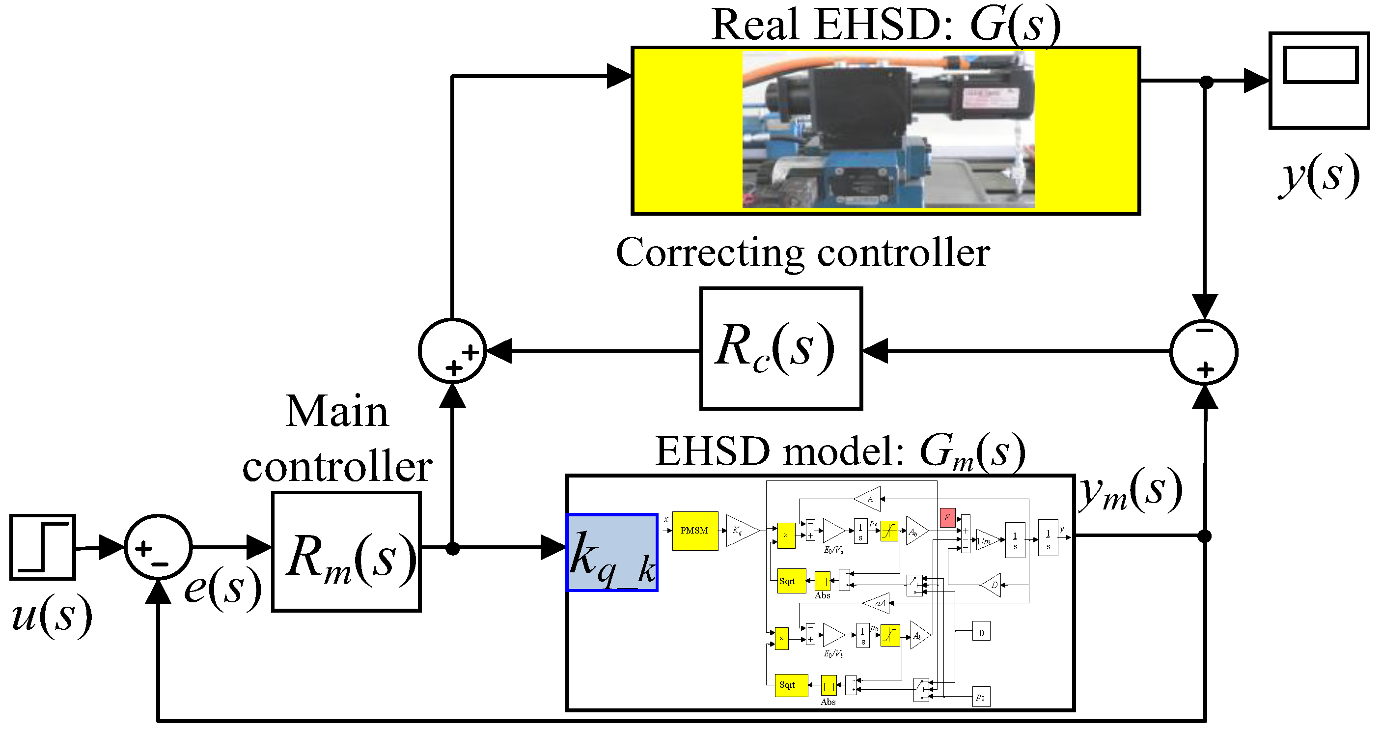The MFC method uses the model-based control [10,11,12], in which part of the control system is a simulation model of the controlled device or process. The classic MFC system appeared in the literature in the early 1990s. Its block scheme diagram is shown in Figure 1. The construction of this control is based on two regulators: R_m, which controls the model of the plant, and R_c, which corrects the model inaccuracies of the simulated loop and handles other disturbances. In this concept, there are two loops, i.e., the model loop R_m–G_m and the process loop R_c–G. The first of them is created by the model of a controlled object and the linear controller type P, PI, or PID. The regulator R_c is used for the calculation of the real object control signal correction. This regulator uses the difference between output signal of the model y_m and the output signal of the real object y. The model of the object is most often created using experimental tests or through theoretical analysis. Applied in the process loop main regulator, the R_m uses the error signal, which is the difference between the input signal u and the model output signal y_m, for generation of the object control signal. In the model of an electrohydraulic servo drive (EHSD), there is a coefficient k_{q_k}, which increases the flow factor of the drive reference model.

Based on the MFC method block scheme presented in Figure 1, the servo drive output signal can be written as follows:

$$y_{MFC}\left(s\right)=\frac{R_m\left(s\right)G\left(s\right)\left[1+R_c\left(s\right)G_m\left(s\right)\right]}{\left[1+R_m\left(s\right)G_m\left(s\right)\right]\left[1+R_c\left(s\right)G\left(s\right)\right]}u\left(s\right)+\frac{1}{1+R_c\left(s\right)G\left(s\right)}z\left(s\right)$$

(1)

where u(s)—input signal, G(s)—transfer function of controlled object or real drive, R_m(s)—main regulator, G_m(s)—model of the controlled object, R_c(s)—correcting regulator, y(s)—output signal, and z(s)—disturbance, i.e., load.

The second component of Equation (1) describes the disturbance signal influence on the output signal. The advantage of the MFC method is that the load influence may be reduced by a regulator R_c. If in both loops the same linear controller is applied [13], i.e., R_c(s) = R_m(s) = R(s), Equation (1) reduces to

$$y_{PID}\left(s\right)=\frac{R\left(s\right)G\left(s\right)}{1+R\left(s\right)G\left(s\right)}u\left(s\right)+\frac{1}{1+R\left(s\right)G\left(s\right)}z\left(s\right)$$

(2)

The main test of MFC application is to force the controlled object to act as an assumed model G_m(s), which may be modeled by expected, desired transfer function. The control procedure of the MFC method aims to reduce the differences between the controlled system and the model to zero.

Taking into account the principle of operation of the proposed system, a step function signal will never occur on the input of the correcting regulator. This makes it possible to fine-tune the correction regulator such that greater stability reserves are obtained (for example, with a higher gain value coefficient). Thanks to this, the control system can make more effective correction of different kinds of disturbances.

Much research has been carried out over the last 20 years to apply the model-following control method in different devices and processes. Tyler, in 1964 [11], applied quadratic optimal control to synthesize model-following control systems. Erzberger, in the study [12], presented the analysis and proposed design criteria for different configurations of models to be followed in the MFC. Durham, in [13], included a review of methods used to solve linear model-following problems, and gave an introduction to recognize methods which may be applied in solving nonlinear systems.

A model-following control of robots has been widely investigated in many institutions, and several variations and practical applications of this method are described in the literature. An example is the variable structure model-following control method, in which the precise system model is generally not required. This approach is proposed and discussed in [14]. To overcome the difficulties in robot control, an adaptive robust model-following control was implemented and described in [15]. Leung et al., in [16], investigated an adaptive variable structure model-following control. In paper [17], the adaptive model-following controller was applied to relieve the difficulty of selecting the switching point in time-optimal tracking control. The controller was applied to the tracking actuator of a magneto-optical disk drive to improve its slow tracking performance.

In article [18], the described research is focused on the two-loop control structures containing a model of the controlled object and two PID controllers. The robustness of plant parameter perturbations and sensitivity to disturbances are investigated. The proposed MFC systems can be applied to robust control of objects with varying parameters. The robust tracking and MFC application for a class of linear dynamical systems with time-varying uncertain parameters and disturbances is considered in [19]. The proposed robust tracking controllers enable the tracking error reduction to zero. A procedure for designing such a controller is introduced along with a numerical example to validate the results. Tsang and Li, in [20], proposed a robust nonlinear nominal-model-following control, which is used to overcome dead zone nonlinearities. The controller contains an ordinary PID controller combined with a dead band relay. It is practically used to control a DC motor position servo system containing dead-zone nonlinearity. Both simulation and experimental results have shown the effectiveness and robustness of the proposed technique. Another interesting application of a model-following approach for control of a DC motor is presented by Rashidib et al. in [21]. The sliding mode observer is used to estimate the state variable of the friction model. A model reference adaptive control system is designed to track the desired speed trajectory while alleviating the adverse effects of model uncertainties and friction. In this control system, the estimated values of the friction state and parameters are given.

One of the first attempts to apply the adaptive model-following control in electrohydraulic drives is described in [22]. This method was derived based upon Lyapunov’s direct method with a goal to obtain better performance of the drive. To deal with the nonlinearities and with the unknown disturbances that are associated with the electrohydraulic drive dynamics, the use of a small ultimate bound of the state error as an adaption criterion is proposed. In the paper, only simulation investigations are described, which demonstrated the effectiveness of the controller.

Sugai and Nonami presented, in paper [23], the hydraulic mine detection hexapod robot, which should achieve a high trajectory tracking performance. The reference model-following sliding mode controller has been designed, which combines the advantages of control theories. As shown in the paper, the proposed control method can improve the trajectory tracking performance and robustness.

In paper [24], a model reference adaptive controller is designed and used to control the position of a servohydraulic variable piston motor. The time response of Bessel’s third-order filter is chosen as the reference model. The obtained experimental results of the drive with the PID, the proportional model-following, and the model-following optimal controller are compared with results obtained when the adaptive controller is used.

Nishiumi and Watton proposed, in [25], the incorporation of a model reference adaptive control scheme, in which an artificial neural network is used as the feedback compensation element of an electrohydraulic servo drive speed control system. The objective was to adapt the feedback loop of this network using an appropriate reference model. It seemed that the acceleration feedback emulation made by artificial neural network is possible, which improved the drive dynamic behavior and removed the steady state error.

In paper [26], a new approach to designing an adaptive PID controller for the hydraulic crane was investigated. The method depends on comparing the linear model reference response with the nonlinear model response and feeding an adaptation signal to the PID control system to eliminate the error in between. It is found that the proposed method provided the most consistent performance in terms of rise time and settling time regardless of the nonlinearities. The demonstrated simulation investigations have shown that the proposed control method can be implemented in the hydraulic crane. The obtained results showed that the used controller exhibits much better response parameters, much better tracking characteristics, and assures very good following motion properties comparable to, or better, than those obtained by the conventional optimally tuned PID controller.

In article [27], a predictive position control method, based on a input-constrained nonlinear dynamic model, is proposed. The method was applied to control a planar motor. The advantage of the proposed method is, among others, to represent dynamic systems with nonlinearity, good coupling, and control input constraint. Similar to the presented method, in the MFC controller, the model can be linear, which facilitates its implementation.

In the paper [28], the authors proposed a multiple-vector direct model-predictive power control method for the grid-side power converter control of a back-to-back converter PMS generator wind turbine system. The control system was implemented in the FPGA circuit. The method is an interesting alternative to the MFC method and can potentially be implemented in an electrohydraulic system. The use of FPGA could additionally increase the operating frequency of the steering system, which could be significant if an electrohydraulic servo valve with a torque motor with a small-time constant was used as the setting element.

Another method that can potentially be used in hydraulic systems is described in paper [29]. Authors proposed a model-predictive control scheme for dual-output matrix converter. Methods from the group of model-predictive methods are indicated as an alternative to the MFC control system.

Another article [30] presents a finite control set model-predictive control strategy for a single-input dual-output indirect matrix converter. This is another example of a method from the model-predictive control (MPC) group.

In publication [31], authors proposed an adaptive fixed-time controller, based on disturbance compensation technology, to achieve high-efficiency position precision control for a magnetic levitation system. The proposed system has the advantage of improving steady-state performance without losing dynamic efficiency. It may find potential use in hydraulic systems.

An example of robust adaptive control is shown in the publication [32], where this technique was used for an electrohydraulic drive. This method is an interesting alternative to the MFC method, and its advantage is that it does not require tuning of the regulator.

Authors of [33] proposed the generalized proportional integral observer-based dynamic prescribed performance sliding mode control method for a DC–DC buck converter with disturbance to achieve high output voltage tracking performance. Simulation and experiments were performed.

There are two main difficult steps, which should be made during the design of an MFC control system:

(a)

Identification of the object for the main loop.

(b)

Tuning of PID controllers’ parameters for both regulators.

A solution for these tasks is crucial for the effective work of the described control system. The developing of an MFC controller for an electrohydraulic servo drive requires the following actions:

-

Building the model of the electrohydraulic drive G_m(s) for the main control loop.

-

Identification of parameters for this model.

-

Application of the PID controller R_m in the closed loop.

-

Finding of the PID parameters.

-

Adding the correcting control loop.

-

Changing the parameters of correction regulator R_c(s) to compensate for the load.

All the above-mentioned steps should be performed in the same working conditions, i.e., pressure, temp, load, etc. The regulators used in the MFC and PID are described by the following equations:

$$u_{Rm}\left(t\right)=k_p\left[e_y\left(t\right)+T_i{\int }_0^t{e}_y\left(t\right)dt+T_d\frac{d{e}_y\left(t\right)}{dt}\right]$$

(3)

$$u_{Ro}\left(t\right)=\underset{\_}{k_{ko}}\times k_p\left[e_y\left(t\right)+T_i{\int }_0^t{e}_y\left(t\right)dt+T_d\frac{d{e}_y\left(t\right)}{dt}\right]$$

(4)

where u_Rm—output signal from model regulator R_m, u_Rc—output signal from correction regulator R_c, e(t)—control error, k_p—gain coefficient of model regulator, T_i—integration time constant, T_d—derivative time constant, k_ko—correcting gain coefficient.

Compared with the other control strategy, the benefits of the proposed method are:

-

A simple two-loop structure.

-

Simplicity of implementation in the embedded systems, including industrial PLC controllers.

-

The possibility of using linear reference models.

The method can be used to compensate the nonlinearities of electrohydraulic servo drives. In the above-mentioned publication [34], the authors conducted a study using the MFC method to compensate for the impact of changing the supply pressure. These were only preliminary and simplified studies. In the present paper, the authors focused on load compensation as a key application for electrohydraulic drives.

3. The Model of Electrohydraulic Servo Drive with the Valve and PMSM Motor

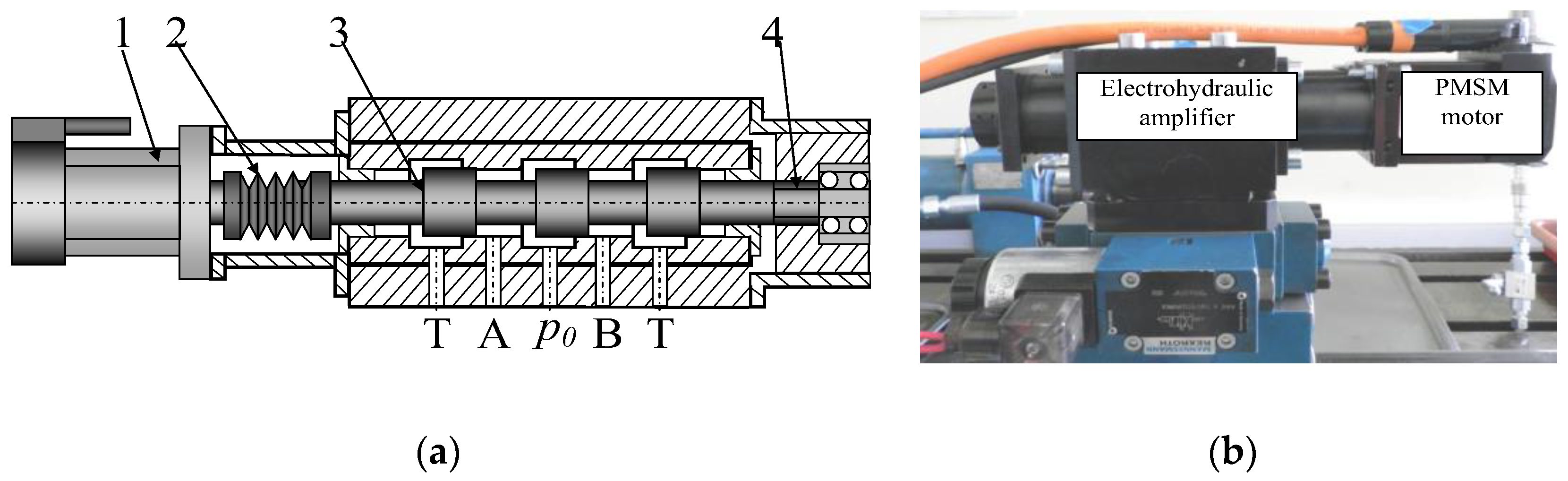
In the last 20 years, the prices of modern synchronous motors and their controllers have decreased significantly. This is due to both the development of modern microcontrollers and improvement of PMSM production technology [35,36]. Therefore, nowadays it is possible and rational to use them in applications where 15 years ago this would not have been economically profitable. Modern synchronous motors can ensure both high positioning accuracy and high dynamics, i.e., acceleration and velocity. In the valve proposed in this paper (Figure 2), the spool is actuated by a low-power PMSM. The valve presented here has been described in detail by the authors in [7].

The synchronous motor (1) is connected to the valve spool (3) using a flexible bellows clutch (2). Thanks to this, applying the supply power to the motor causes its rotation and simultaneously axial translation of the valve spool. The pitch of the screw was 2.5 mm, and the rotor position resolution was 21,600; thus, the minimum spool displacement (position resolution) was 0.12 μm. The valve spool translation x is proportional to the angular motor position changes and to the pitch of the used thread (4). The spool translation causes the proportional valve flow gaps opening or closing.

In the valve proposed here, the low-power commercial PMSM motor [37] is applied. Taking into account the electrohydraulic valve requirements, in the selection of the motor, its high dynamics and small size were of key importance. The PMSMs basic parameters are:

-

Power: 105 W.

-

Rated speed: 3000 rev/min.

-

Rated current: 2.9 A and stall torque: 0.680 Nm.

-

Stator windings inductance: 4.1 mH.

-

Resistance of the windings: 2 ohm.

-

Electrical time constant: 2 ms.

The motor was connected to an absolute encoder EnDat, which provided digital (pulse) information about the current rotor position. The encoder resolution was 21,600 pulses per revolution.

As the authors have shown in publications [38], a valve with a PMSM motor has better dynamic parameters than a comparable proportional valve with electromagnets. It is also important that, taking into account the physical implementation on the PLC controller, the electric motor can be directly controlled. The frequency characteristics, including the stability of the valve, are also described in the referenced publication. The valve used in the project is a proprietary design proposed by the authors, the advantage of which is the possibility of using electric motors matched to the superior control system, and rotary motors are more easily accessible.

To implement the MFC method in the above electrohydraulic servo drive, it is necessary to build a model of the proportional valve with a synchronous motor, and after that, the entire drive, based on it.

Because the edges of the valve are sharp, the oil flow through the valve is turbulent [39]. The hydraulic valve oil flow through the hydraulic nozzles can be characterized using a square root equation. These flows can be described by using the following equations:

for: x > 0:

$$\begin{gathered} Q_a\left(t\right)=K_Q\sqrt{p_0-p_a\left(t\right)}\times x\left(t\right) \\ Q_b\left(t\right)=K_Q\sqrt{p_b\left(t\right)}\times x\left(t\right) \end{gathered}$$

(5)

for: x < 0:

$$\begin{gathered} Q_a\left(t\right)=K_Q\sqrt{p_a\left(t\right)}\times x\left(t\right) \\ {Q}_b\left(t\right)=K_Q\sqrt{p_0-p_b\left(t\right)}\times x\left(t\right) \end{gathered}$$

(6)

where x—a valve spool displacement (mm), Q_a—oil flow through the orifice A (dm³/min), Q_b—flow through the orifice B (dm³/min), K_Q—flow gain, p₀—supply pressure (Pa), p_a–pressure in chambers A, and p_b—pressure in chambers (Pa).

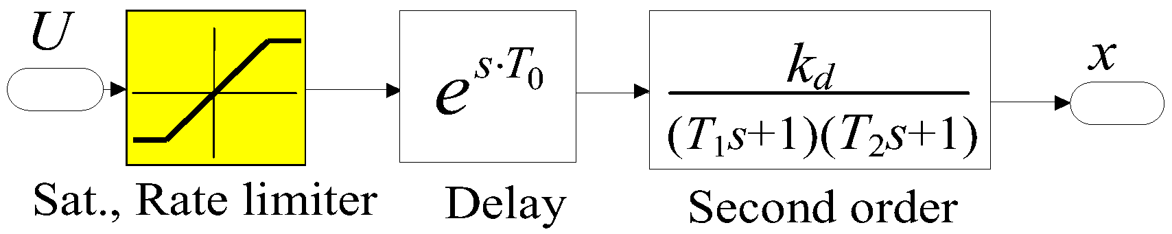
The laboratory investigations made by authors have shown that the synchronous motor used in the valve can be described in simple terms by a second-order transfer function with delay [7]:

$$G(s)=\frac{X(s)}{U(s)}=\frac{k_d\cdot e^{s\cdot T_0}}{(T_1\cdot s+1)\cdot (T_2\cdot s+1)}$$

(7)

where k_d = 2.5—the gain coefficient, T₀ = 0.01 s—transport delay, and T₁ = 0.0030 s and T₂ = 0.0015 s—time constants.

However, in a real motor, signal rise rate is limited and saturated to the maximum supply current of the motor windings. Therefore, the nonlinear block with “rate limiter” and “saturation” are added to the model. The model is described in detail in [38]. It is presented in Figure 3.

The model of the electrohydraulic servo drive is built basing on the theoretical description of the hydraulic drive. The following equations are formulated and used [1,2]:

$$Q_a(t)=Q_{sa}(t)+Q_{ha}(t)+Q_v(t)$$

(8)

$$Q_b(t)=Q_{sb}(t)+Q_{hb}(t)+Q_v(t)-Q_{vb}(t)$$

(9)

$$Q_b(t)=K_{Qp}x(t)-K_l{p}_b(t)$$

(10)

$$Q_{ha}(t)=A\frac{dy(t)}{dt}$$

(11)

$$Q_{hb}(t)=aA\frac{dy(t)}{dt}$$

(12)

$$Q_{sa}(t)=\frac{V_a}{E_o}\frac{d{p}_a(t)}{dt}$$

(13)

$$Q_{sb}(t)=-\frac{V_b}{E_o}\frac{d{p}_b(t)}{dt}$$

(14)

$$Q_v(t)=K_v[p_a(t)-p_b(t)]$$

(15)

$$Q_{vb}(t)=K_{vb}{p}_b(t)$$

(16)

$$m\frac{d^{2}y(t)}{d{t}^2}+D\frac{dy(t)}{dt}=A[p_a(t)-a{p}_b(t)]$$

(17)

where Q_a, Q_b—oil flow from the valve to hydraulic cylinder chamber, Q_ha, Q_hb—absorption of the actuator chambers, Q_sa, Q_sb—flow covering the losses caused by compressibility, Q_vb—leakage flow on the piston rod, p_a, p_b—the pressure in the chambers of the actuator, A, aA—active piston cross section areas on both sides, V_a, V_b—the volume of liquid in the hydraulic hoses and chambers in the actuator, D—kinematic friction coefficient, K_l—coefficient considering the reduction in flow rate caused by the non-zero pressure drop on the piston (linearization of flow characteristics), K_va, K_vb—leakage coefficient on the piston and the piston rod, E₀—bulk modulus of the oil, and m—load mass reduced on the piston.

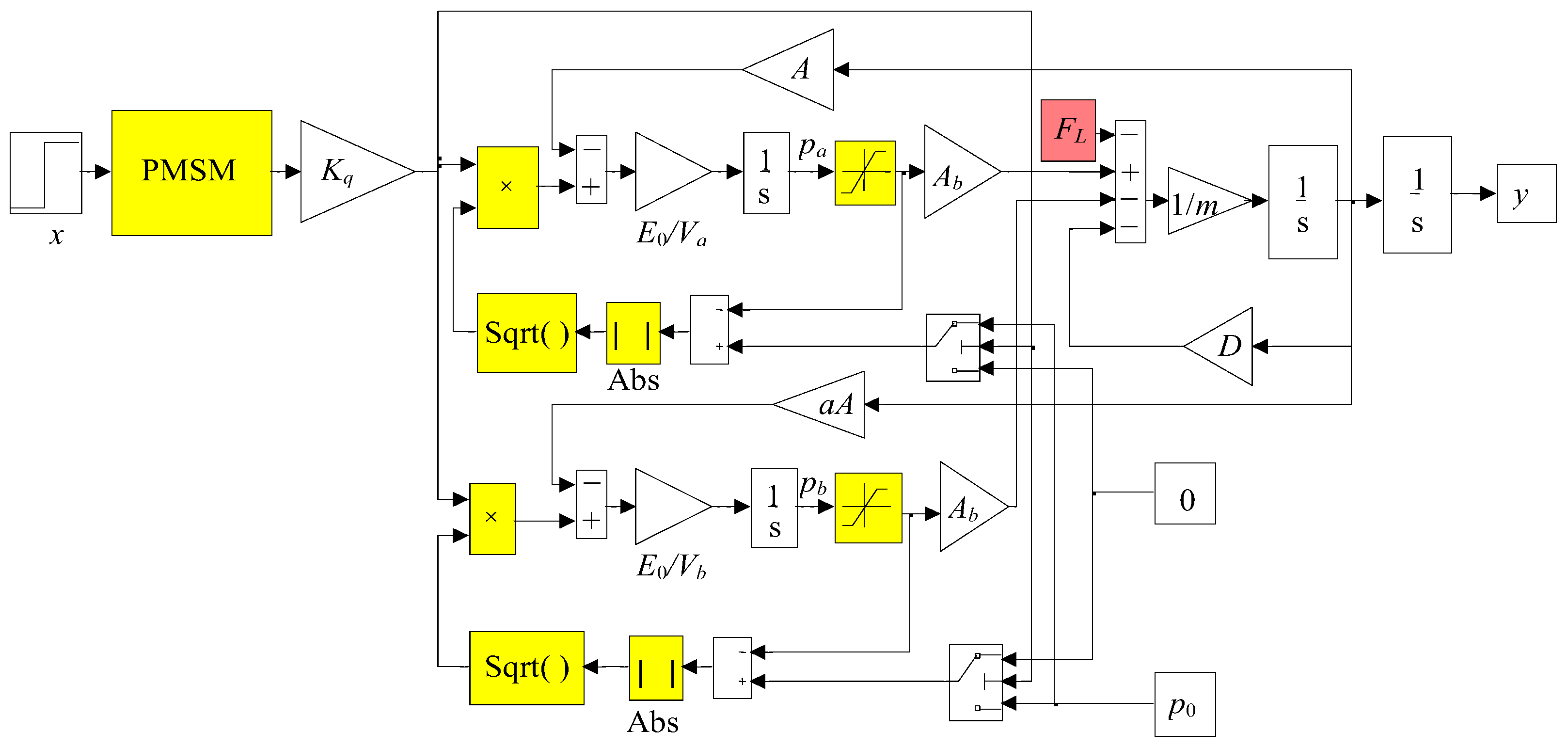
Based on the above Equations (5)–(17), the electrohydraulic drive model was built (Figure 4), in which the proportional valve with PMSM was built. The stroke of the hydraulic cylinder was 200 mm; its diameter of the piston rod was A = 40 mm, and the piston diameter was aA = 63 mm. In the simulation model, the linear stiffness changes in function of piston position are included. Additionally, a linear coefficient of kinetic friction is taken into account, which was estimated as D = 29,000 (N × s/m). The shifted mass of the piston and piston rod reduced on the cylinder piston was m = 20.2 kg. The bulk modulus of the hydraulic oil was E₀ = 1.2 × 10⁹ N/m² [1,2]. The values of the coefficients used in Equations (14) and (15), calculated in the middle position of the piston, amounted to E₀/V_a = 3.82 × 10¹¹ Pa/m³ and E₀/V_b = 5.96 × 10¹¹Pa/m³.

4. Simulation Investigation

Due to the development of simulation research and to compare PID and MFC controllers, the drive and controller models were built in Matlab Simulink (The MathWorks, Inc., Natick, MA, USA). On the input of both control loops (PID and MFC), a step signal was given. Individual coefficients of both regulators were chosen experimentally using the Ziegler Nichols method as k_p = 15, T_i = 0.001, T_d = 0.5. It was assumed that the step response should be characterized by minimal settling time but without oscillations. The multiplication of the correcting regulator gain coefficient was k_ko = 4.

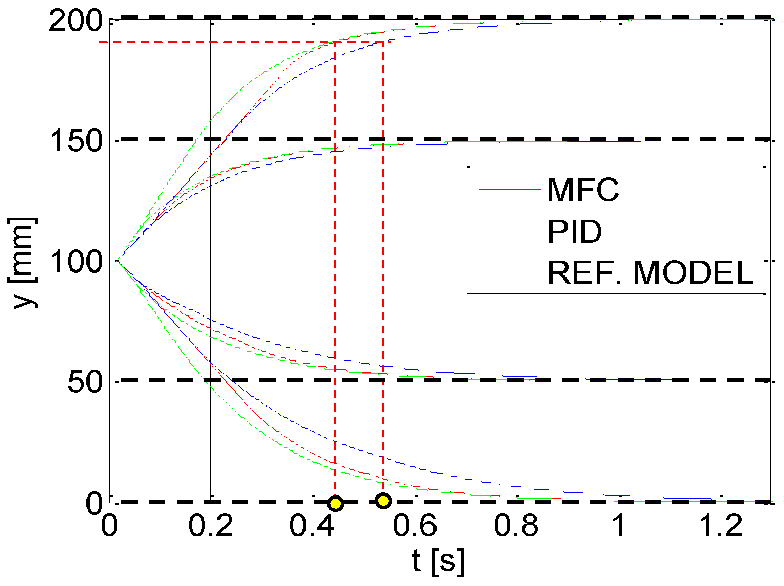
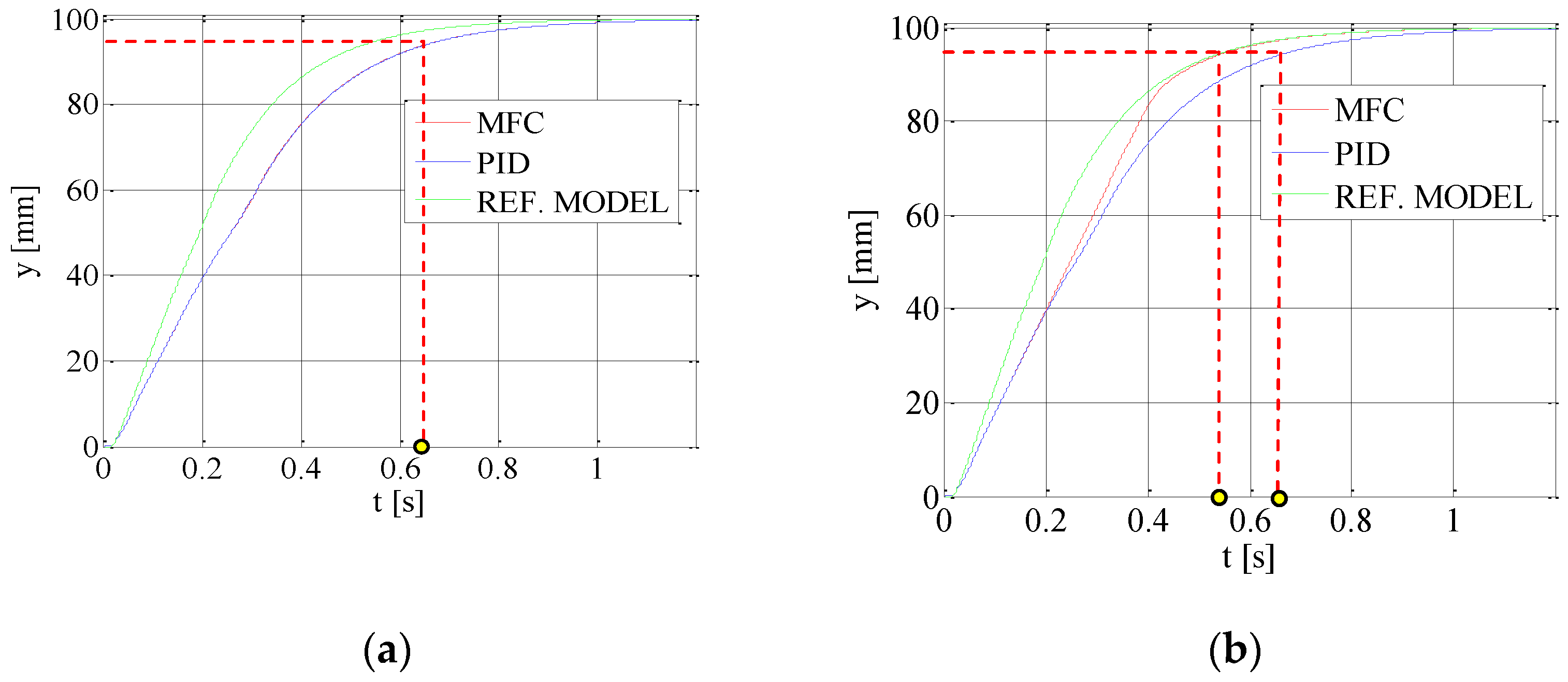
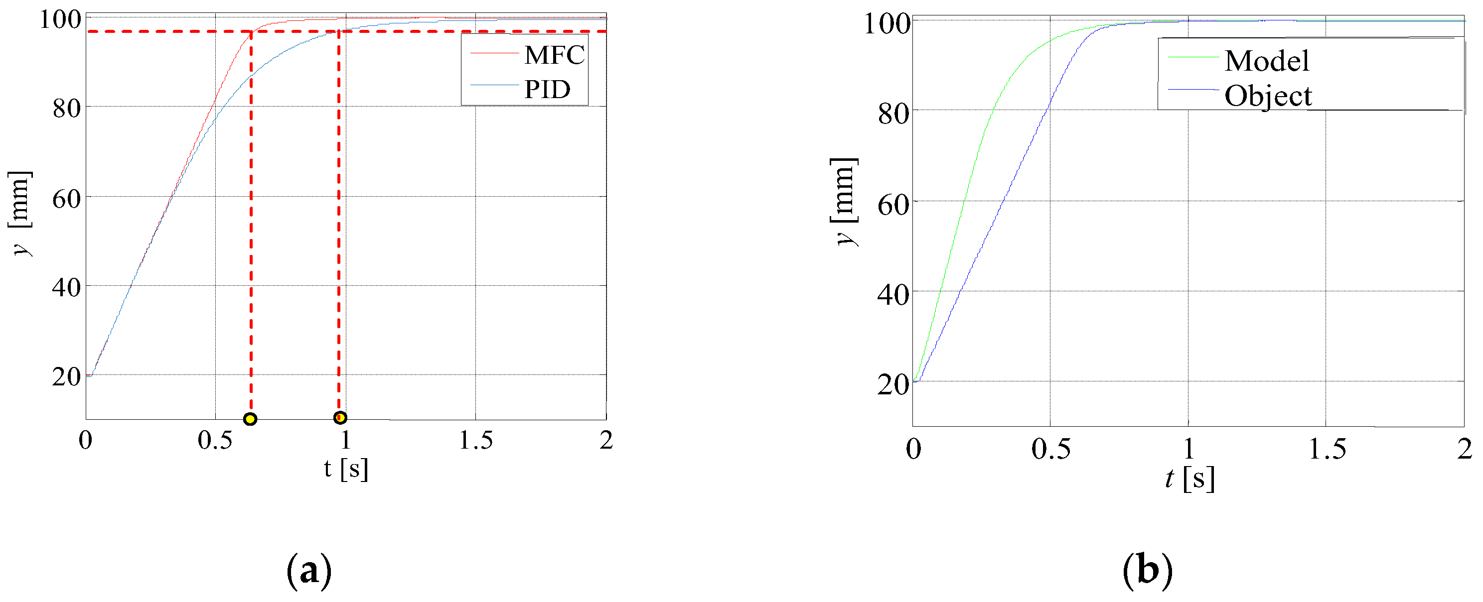
Simulation results, i.e., the recorded step responses, are shown in Figure 5. It has been observed that the compensation works well for different set points. The settling time for the drive controlled by MFC was about 0.44 s and for the PID it was 0.56 s (yellow points in Figure 6).

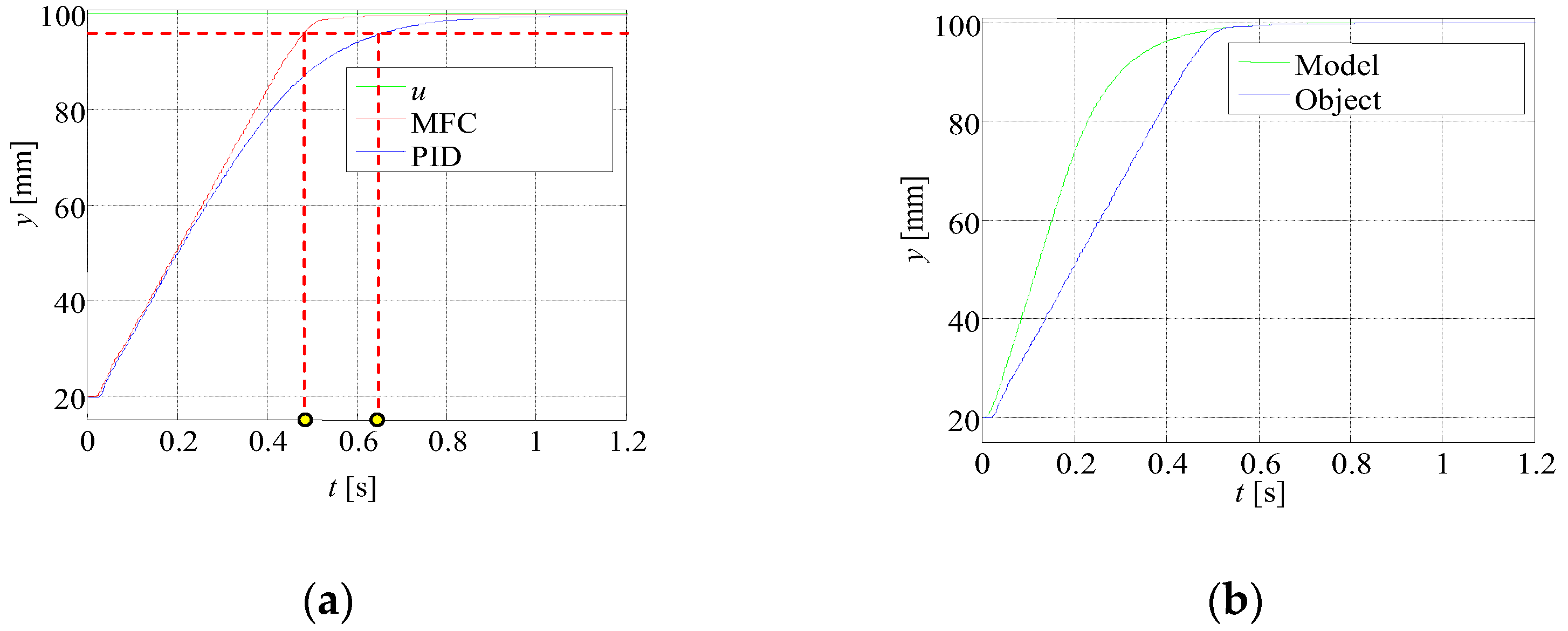
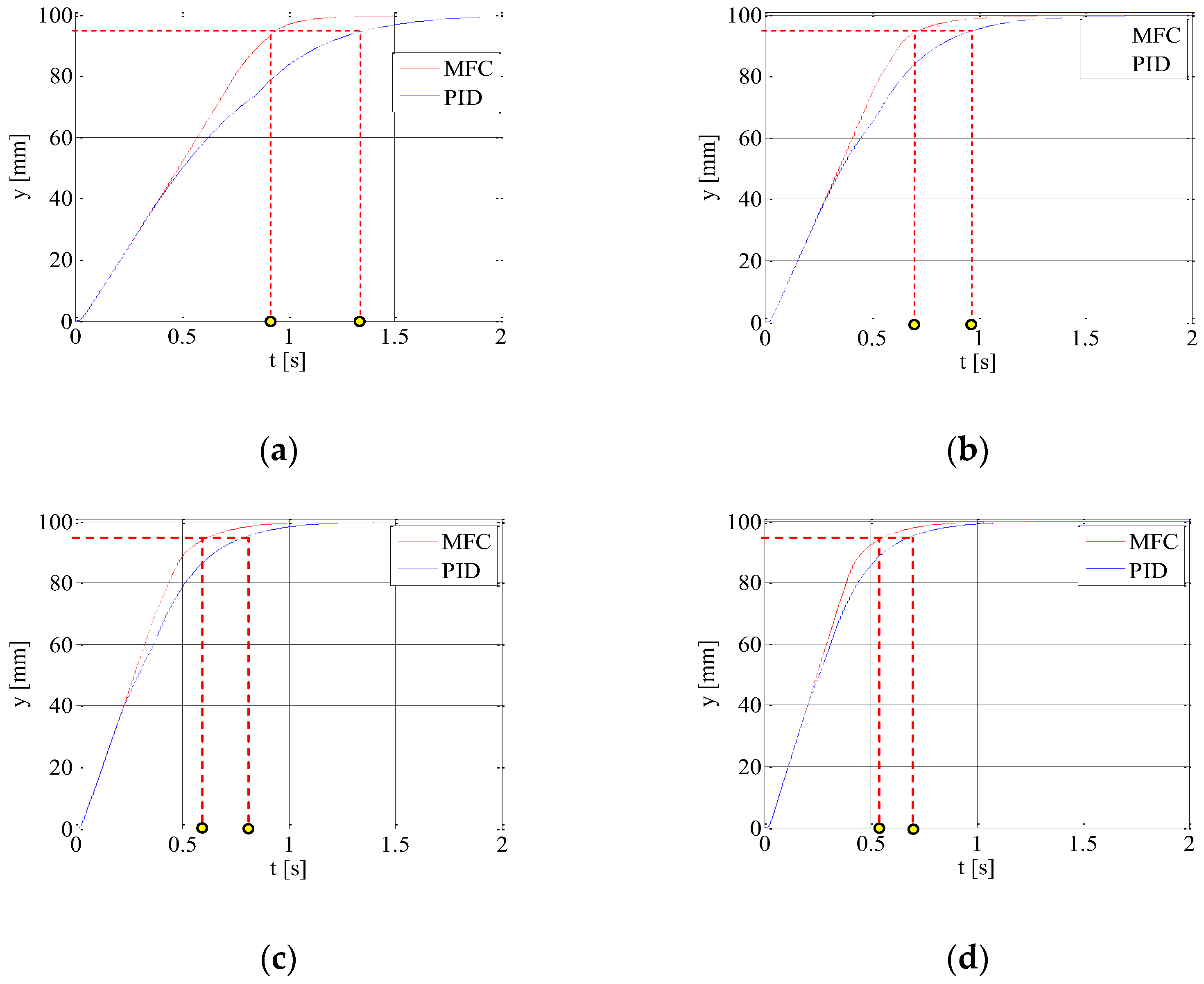
In the next steps, the results of the research on changes in selected controller parameters for the selected set position value are presented. The impacts of the load changes are shown in Figure 6. The load in the described control system is treated as a disturbance. The settling time for MFC was about 0.52 s and for PID it was 5.65 s.

The method could also be successfully used in the event of a change in the drive supply pressure, as shown in Figure 7.

The impact of individual controller parameters for both loops is shown in Figure 8.

The proposed controller, based on the MFC method, allowed a change to the flow coefficient K_Q in the reference model, multiplying it by k_{q_k} coefficient (Figure 1):

for: x > 0:

$$\begin{gathered} Q_a\left(t\right)=K_Q\times k_{q_k} \sqrt{p_0-p_a\left(t\right)}\times x\left(t\right) \\ Q_b\left(t\right)=K_Q\times k_{q\_k}\sqrt{p_b\left(t\right)}\times x\left(t\right) \end{gathered}$$

(18)

for: x < 0:

$$\begin{gathered} Q_a\left(t\right)=K_Q\times k_{q_k}\sqrt{p_a\left(t\right)}\times x\left(t\right) \\ {Q}_b\left(t\right)=K_Q\times k_{q\_k}\sqrt{p_0-p_b\left(t\right)}\times x\left(t\right) \end{gathered}$$

(19)

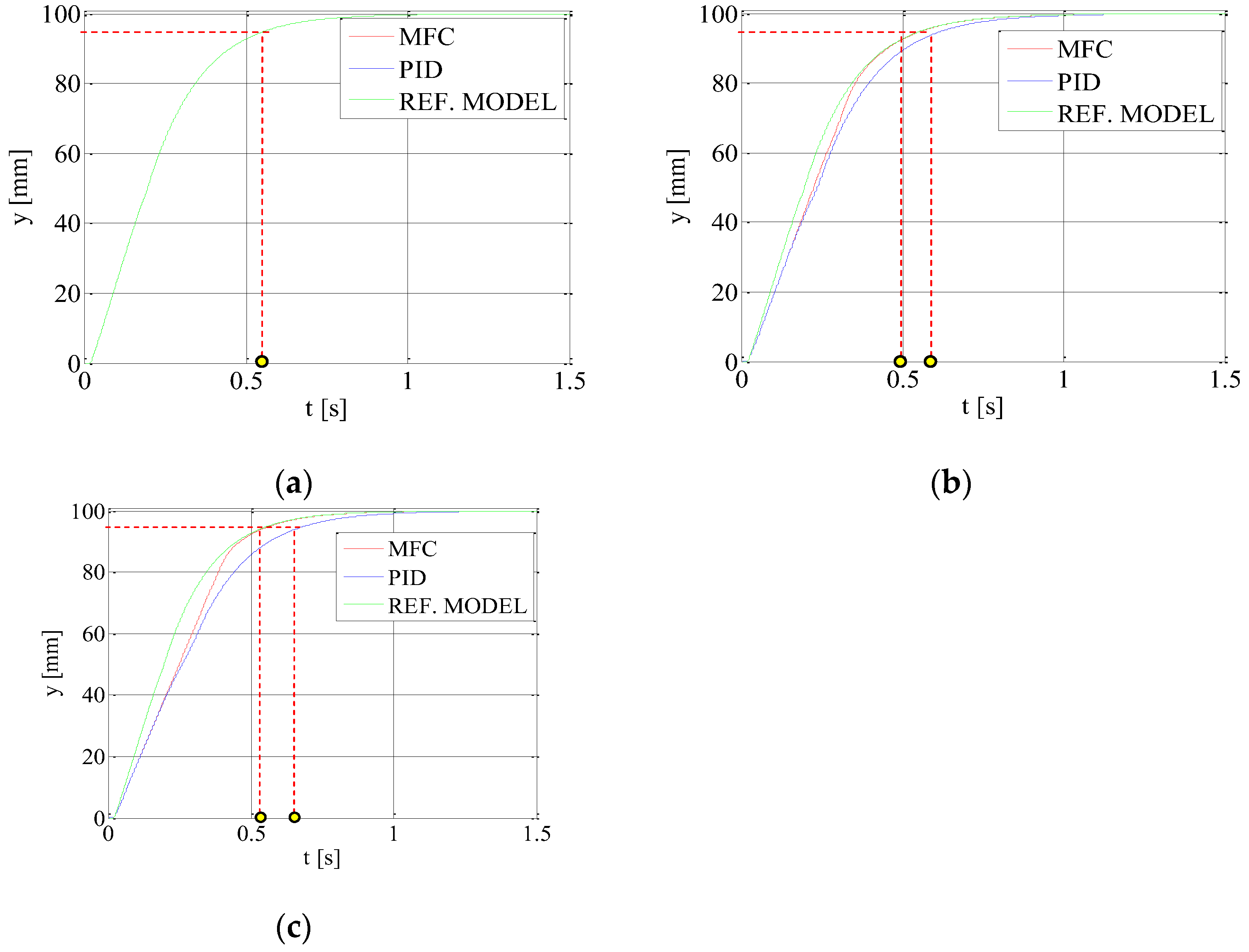
Change of this coefficient improved the dynamics of the model. The MFC regulator trends to tracking the reference model, which resulted in an improvement in the dynamics of the whole system.

Figure 9 shows the effect of changing this parameter if the corrective controller and the model controller have equal values. Changing this parameter in the described case improves the dynamics by shortening the settling time of the MFC controller in relation to the PID controller by 0.19 s. This is because the real object conforms to a reference model with a greater gain factor.

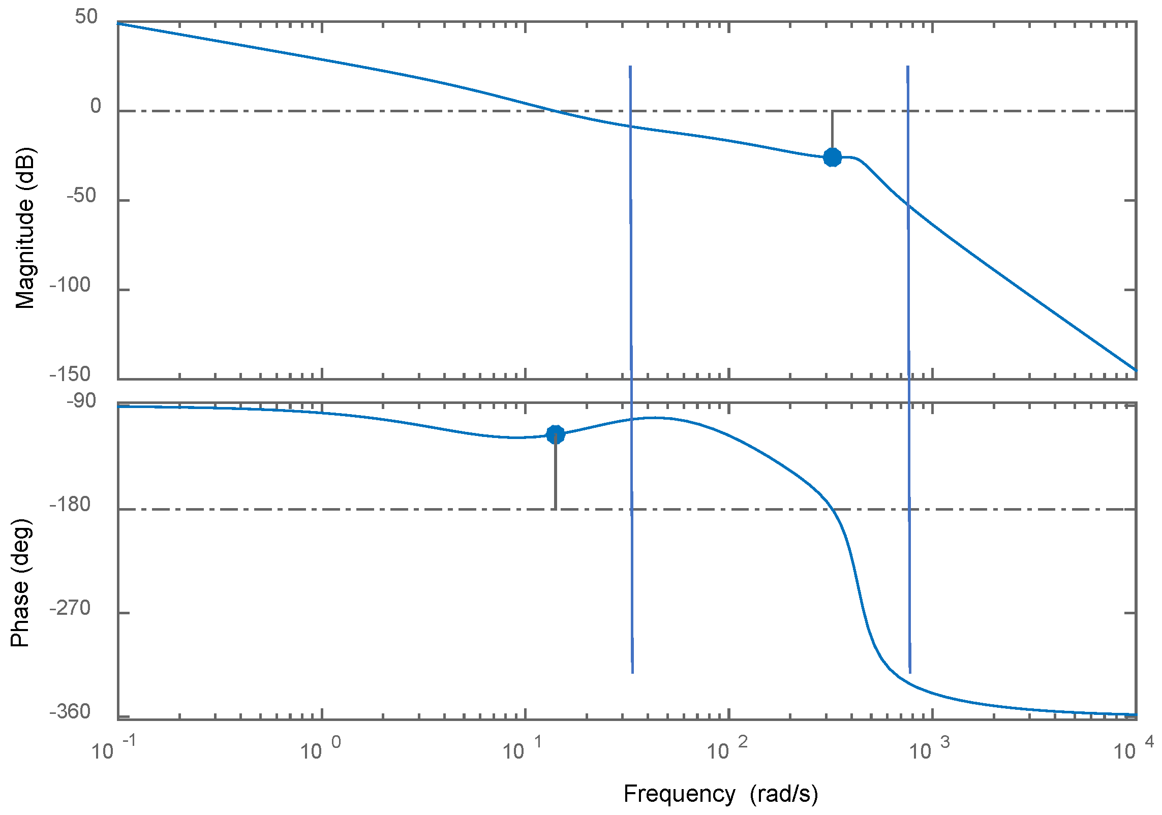
Based on simulation tests, the following stability margins for the electrohydraulic drive with MFC controller were determined (Figure 10):

-

Gain margin (dB): 25.9 (at frequency (rad/s): 323).

-

Phase margin (deg): 65.1 and delay margin (sec): 0.0807 (at frequency (rad/s): 14.1).

Doubling the diameter of the active cross-section areas of both sides of the piston rod causes change of the stability margins to:

-

Gain margin (dB): 42.2 (at frequency (rad/s): 635).

-

Phase margin (deg): 59.9 and delay margin (sec): 0.152 (at frequency (rad/s): 6.87).

On the other hand, doubling the gain coefficient k_p causes change of the stability margins to:

-

Gain margin (dB): 24.4 (at frequency (rad/s): 317).

-

Phase margin (deg): 50.7 and delay margin (sec): 0.0314 (at frequency (rad/s): 28.1).

These examples show that the developed system is resistant, i.e., stable, despite changes in various parameters.

5. Investigations and Discussion

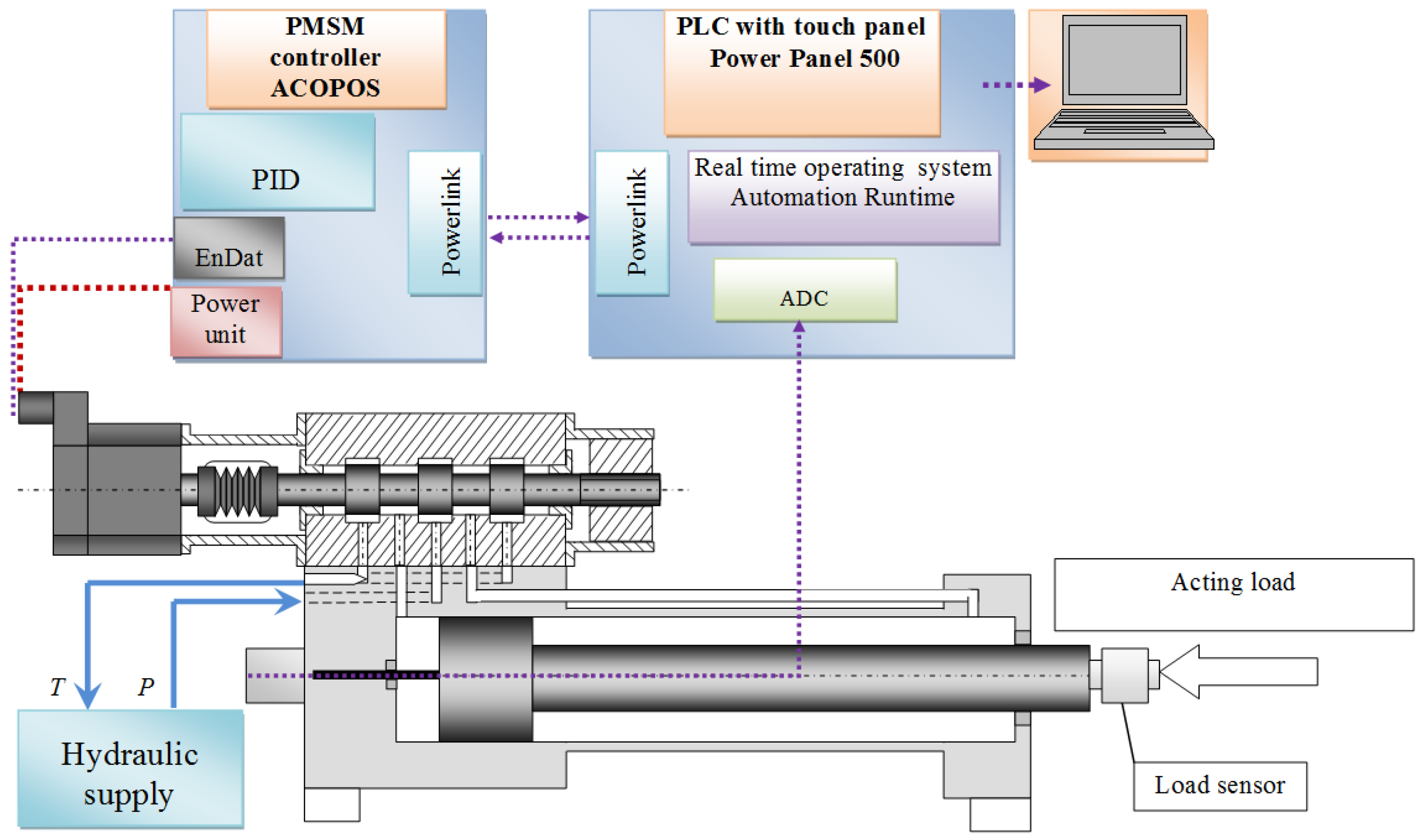
In Figure 11, the structure of the laboratory test stand that was built is presented. The stand allows us to check the effectiveness of the load disturbances compensation if the proposed controller based on the MFC method is used. On the test stand, a single-acting cylinder with a proportional valve controlled by PMSM is installed. As a control unit, a PLC was used. The cylinder piston position was measured by the assembled sensor, which was a magnetostrictive sensor, built inside the cylinder. Its output signal was the voltage ±10 V. A control system was based on a master controller, consisting of a PLC with a touch panel. The motor was controlled by the servo-inverter, which acted as a slave controller. The PLC enabled real-time control, and the system worked with a cycle frequency of 1250 Hz.

The electrohydraulic drive was supplied by a hydraulic power unit, which kept the pressure constant. The valve with the PMSM motor controlled the hydraulic piston displacement, changing the pressures in cylinder chambers and flow of oil from the supply unit to the actuator chambers.

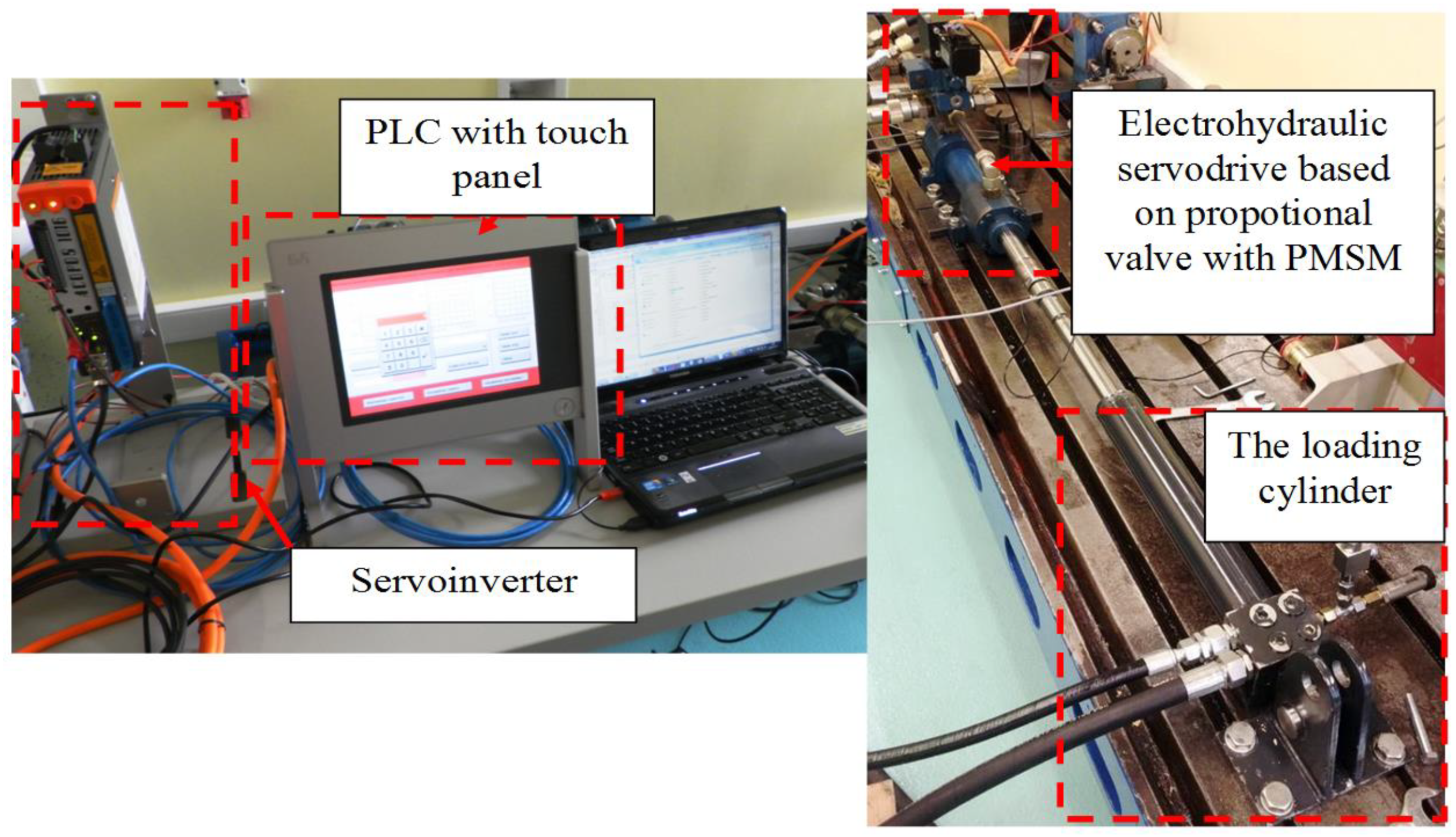
The test stand was equipped with the load electrohydraulic cylinder and force sensor type HBMC9B, which allowed us to measure the force up to 50 kN (Figure 12).

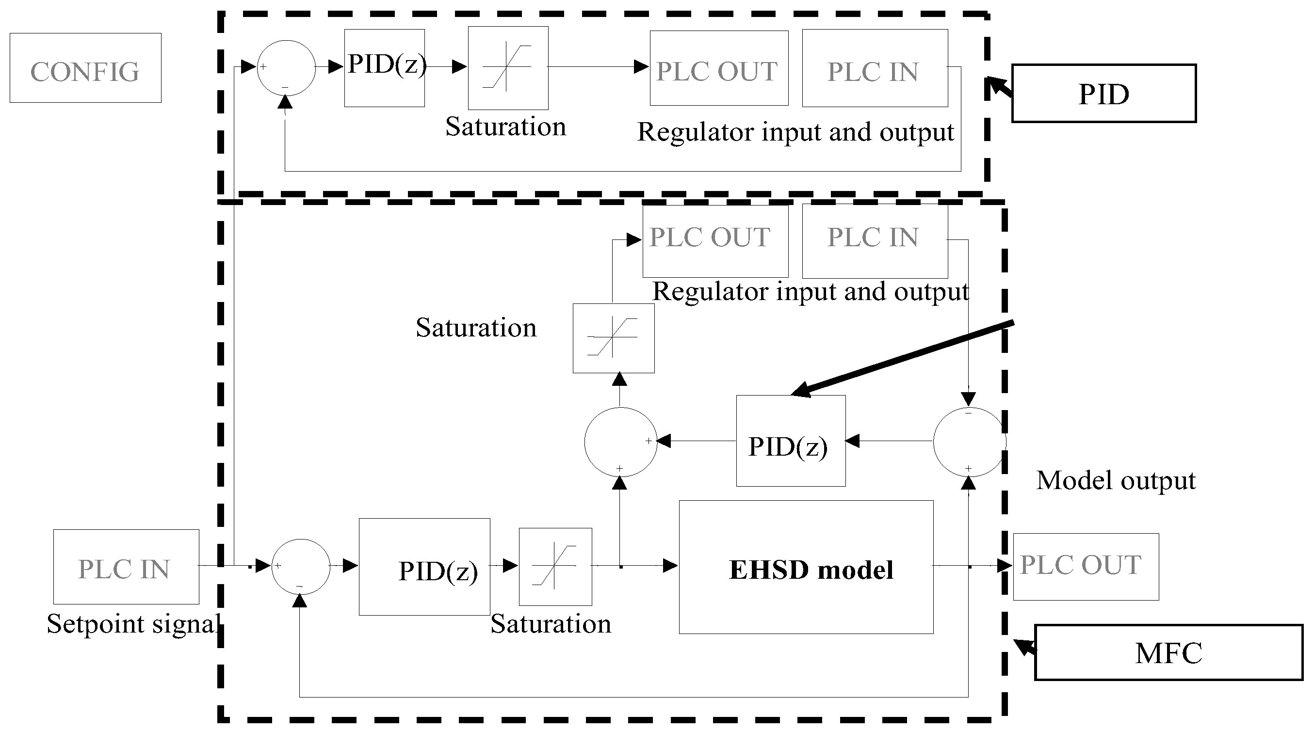
The model of the drive is implemented in the model loop of the MFC controller (Figure 13). The software implemented on the PLC control enabled to switch between a PID and MFC controller. In the design of the control system, the rapid prototyping technique for the control system design is used. In this approach, the model of the control system has been built previously in the software environment and improved. After obtaining positive test results, it was recompiled for the C code and then implemented as one of the task classes in the PLC. Because the used industrial controller PLC worked in a discrete mode, it was necessary to discretize the continuous model of the control system. The discrete time base was established as T = 0.8 ms. This value resulted from the minimum time base for a single task execution on the PLC controller.

PID and MFC controllers for electrohydraulic servo proportional valve with synchronous motor were tested and compared using drive step responses. The parameters of all used PID controllers were established experimentally as follows: k_p = 15, T_i = 0.001 s, and T_d = 0.5 s. In order to achieve the improvement of the tested electrohydraulic drive dynamics, the gain coefficient of MFC controller R_c(s) was increased from k_ko = 1 to the value of k_ko = 4. If this value is larger, the oscillations occurred in the system. The additional flow coefficient of reference model k_{q_k} was equal to 1.2.

The aim of the applied model-based controller in the electrohydraulic servo drive was to improve dynamic parameters. The load measurements were performed using a force sensor located between the drive rod and piston cylinder loading (Figure 14, Figure 15 and Figure 16). Tests were performed for the hydraulic pressure supply p₀ = 4 MPa, 8 MPa, and 12 MPa.

The graphs show the improvement in the dynamics of operation of the real electrohydraulic drive by reducing the time for obtaining the results. The results are summarized in

Table 1. Settling time comparison.

Controller	Pressure Supply p0 (MPa)	Load F (N)	Settling Time (s)
MFC	12	1800	0.4
PID	12	1800	0.65
MFC	8	1477	0.5
PID	8	1477	0.8
MFC	4	697	0.7
PID	4	697	1.2

. This improvement, i.e., the reduction of settling time for the MFC method, is mainly due to the use of a reference model with an increased gain parameter in the system.

The collected data were also used to compare the applied controllers using the integral absolute error method.

$$I_m={\displaystyle \underset{0}{\overset{\infty }{\int }}|e(t)|dt}$$

(20)

where I_m—IAE (integral absolute error), and e(t)—error.

The mechanical power used by the servo drive during step responses was calculated based on obtained settling time. It can be directly translated into energy consumption assessment. The obtained results are summarized in

Table 2. IAE and mechanical force comparison.

Controller	Pressure Supply p0 (MPa)	Load F (N)	IAE	Mechanical Power (W)
MFC	12	1800	0.0167	342.0
PID	12	1800	0.0190	210.5
MFC	8	1477	0.0207	224.5
PID	8	1477	0.0238	140.3
MFC	4	697	0.0271	75.7
PID	4	697	0.0311	44.1

. It is visible that the shortening of the response time leads to an increase of power generated by the drive. The energy consumption is, in all cases, very similar.

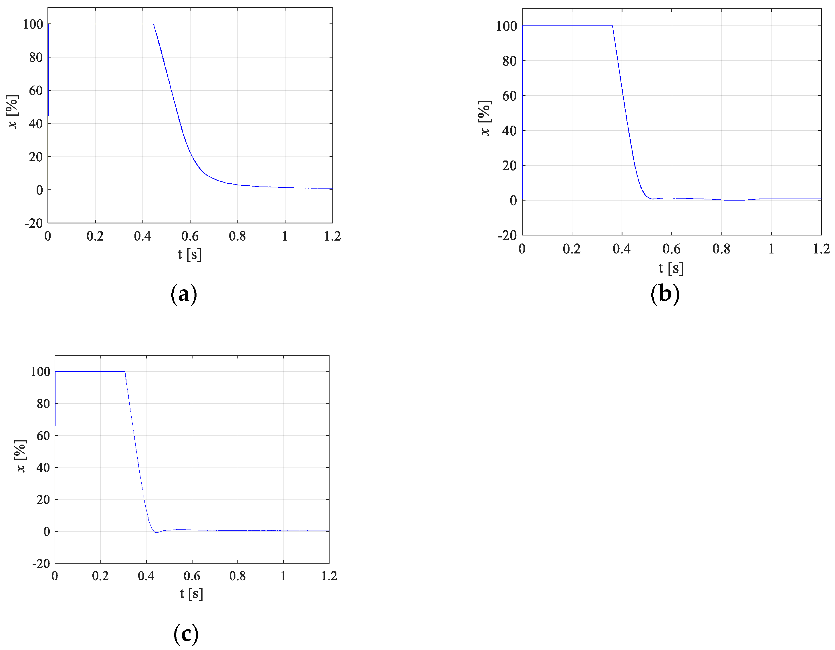
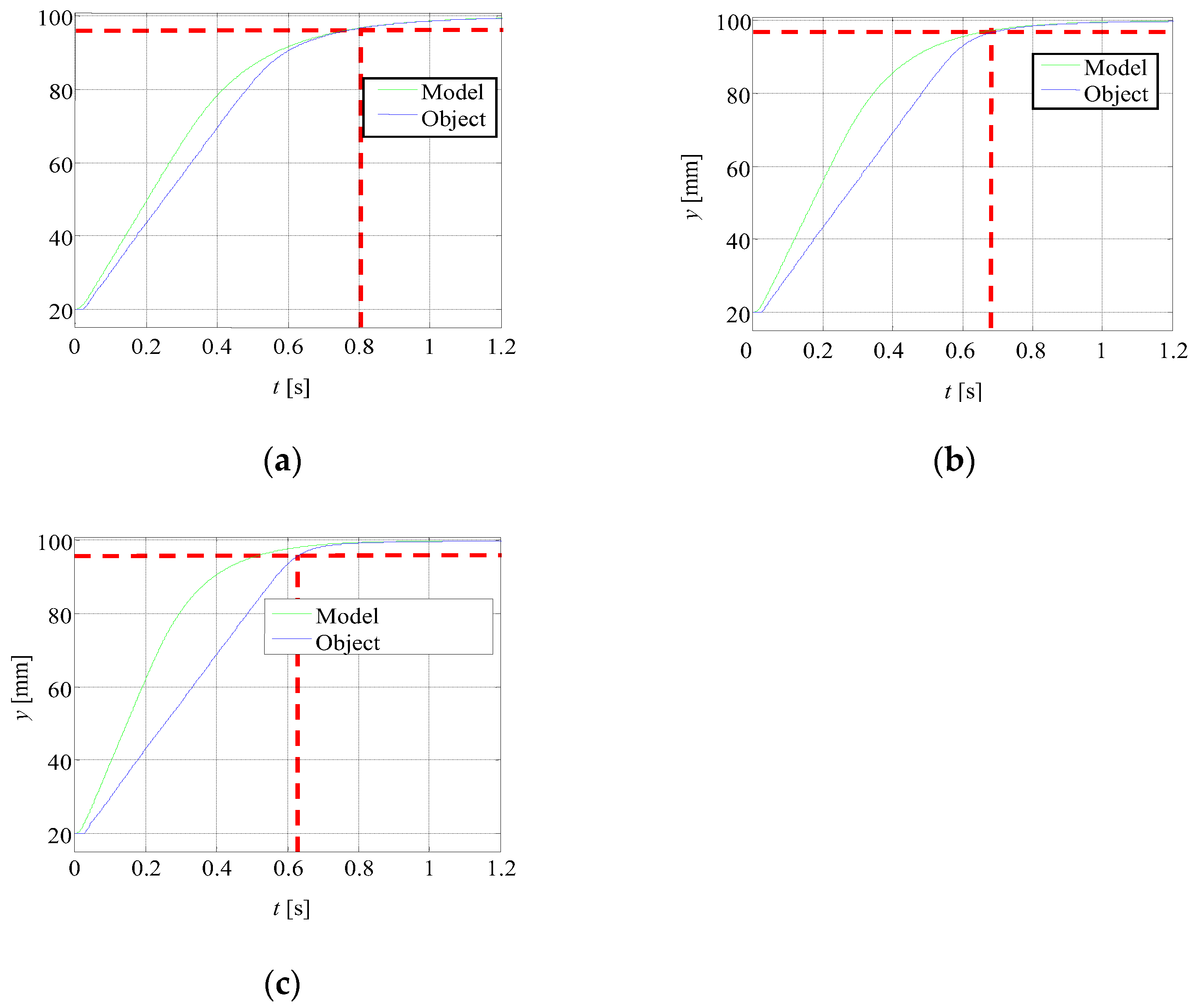
Figure 17 shows the valve spool displacements due to the cylinder piston rod being moved. Increasing the supply pressure increases the dynamics of the spool movement.

In the following studies, the effects of varying model parameters on the control system were investigated (Figure 18). Based on the collected charts, it can be said that faster system responses occur when a reference model in the controller MFC has great rate of the flow, K_Q, of the reference model.

6. Conclusions

The MFC method is usually used in devices or process control when the automatic adjustment is required. The research results presented in this paper were made to verify the MFC method’s usefulness in electrohydraulic servo drives.

The main advantage of the MFC method described above is simplicity of the controller structure in comparison with other modern advanced controllers, such as, for example, adaptive controllers. A model for the main control loop is not very complicated, i.e., based on typical PID. Furthermore, the identification of the controlled object’s dynamics is based only on the time characteristic. Although the nature of the MFC method is linear, it can effectively control the nonlinear objects such as electrohydraulic servo drive. Considering the obtained characteristics, the authors have shown that the MFC method allowed faster correction of external disturbances compared with the classical PID. Based on the calculated mechanical power consumption, it can be concluded that the improvement of the dynamics of the system is related to slightly higher energy consumption. However, proper matching of the drive to the needs of the application will optimize this consumption.

The investigations of the application of the MFC method in electrohydraulic servo drives will be conducted by the authors in the future. Ongoing studies are aimed at designing a control algorithm, which can be implemented in an embedded system. The MFC system offers a much higher robustness to process parameter variations than the classic PID controller.