Displacement-Constrained Neural Network Control of Maglev Trains Based on a Multi-Mass-Point Model

Abstract

To address the safety displacement-constrained control problem of maglev trains during operation, this study applied the radial-based neural network control displacement-constrained method to maglev trains based on the multi-mass-point model, and strictly limited the output of maglev train displacement and speed values to keep the overshoot within a given range. Firstly, the dynamics and kinematics of the maglev train were modeled from the perspective of multi-mass modeling. Secondly, the basic structure of the radial-based neural network was determined according to the displacement-limited constraints of the maglev train during operation, and the stability was proven by applying the control rate and output-limited priming according to the limitations. Finally, based on the displacement-limited operation control of maglev trains, the system of the radial-based neural network was simulated. The simulation results show that this method can make the displacement and velocity signals of the maglev train converge to the command signals, the target convergence position is reached rapidly, and the deviation can be kept within a stable range so that the displacement and velocity signals of the maglev train can be limited to the desired safety constraints, which can guarantee the stability and safety of the maglev transportation system in the operation process.

1. Introduction

To build a new modern comprehensive multi-dimensional transportation travel mode and optimize the existing urban traffic network layout, maglev train systems have an important application value in realizing rapid commuting in cities. The state of the maglev train itself changes with different environments during operation, and it is a prerequisite for the promotion of maglev transportation systems to ensure that maglev trains can travel under a given safe displacement range. If the given safe displacement is exceeded, it will be difficult for maglev trains to guarantee safe and efficient transit; thus, it is important to study the dynamic model of maglev trains through the safe displacement-constrained control method.

Many contemporary scholars have also proposed more dynamic models and control methods for trains. Mao Z et al. [1] studied the adaptive tracking control problem of a multi-body high-speed train dynamics model with unknown parameters and used a feedback linearization method to decompose the system into two-part subsystems in dealing with the nonlinear term problem, proving that the system was stable. Xiaowen Wang et al. [2] proposed an adaptive terminal sliding mode controller (ATSMC) to improve robustness in speed tracking control, and simulations were performed to verify the effectiveness using train data. Y Liu et al. [3] proposed a cascaded predictive fuzzy PID (F-PID) control algorithm with weights, which effectively improved the train tracking accuracy and comfort, and reduced the train’s energy consumption and stopping errors. Qian Pu et al. [4] developed a training model with dynamic parameters considering the time-varying parameters of train motion, combined neural networks with PID algorithms, and verified the effectiveness and stability of this controller. Y Jie [5] used a traction force feedforward approach to address the displacement and speed tracking problem for the time lag of wagon trains, which greatly improved the dynamic performance of the controller. M Chou et al. [6] proposed a longitudinal dynamics model for heavy-haul trains, which was influenced by the input data recorded for a specific track section; the simulation results show that this model was reasonable at considering the speed regulation of heavy-haul trains with electronically controlled pneumatic braking systems and the treatment of internal train forces. J Xu et al. [7] proposed an adaptive robust control method for the levitation control problem of nonlinear maglev trains with state constraints, which allows the air gap to be controlled in a safe range. Sun Y et al. [8] proposed an adaptive neuro-fuzzy sliding mode controller that can suppress disturbances and parameter perturbations in magnetic levitation system controllers in low-speed maglev trains; the design and implementation of this controller significantly reduced the effects caused by parameter perturbations.

Most of the modeling and control objects of the above studies were for high-speed trains. There are fewer studies on the application of maglev trains, and most of the existing studies on maglev train dynamics models focus on single mass points, which cannot accurately reflect the actual situation during operation. In terms of neural network control methods, radial-based neural networks have strong generalization ability and high approximation accuracy, and can automatically increase neurons until they meet the accuracy requirements with a fast convergence speed, which can be applied to the real-time maglev train displacement-constrained control. Therefore, this paper adopts a multi-mass modeling approach. The radial-based neural network control displacement-constrained control was applied to maglev trains, and finally, numerical simulations were performed to demonstrate the effectiveness.

2. Maglev Train Dynamic Model

The prerequisite for research on the displacement-constrained control of maglev trains is establishing an accurate model of maglev train dynamics. In the direction of operation of the maglev train, the forces are traction $F_t(\mathrm{kN})$, braking force $F_b(\mathrm{kN})$ and running resistance $f(\mathrm{kN})$.

2.1. Maglev Train Traction and Braking Force

Traction and braking forces are prerequisites to ensure the proper operation of maglev trains on a guide track. To achieve the safe and efficient operation of maglev trains under normal operation, it is necessary to dynamically adjust the traction and braking forces according to the running speed of maglev trains. When the train speed reaches a certain value, the traction force needs to be reduced, and the braking force needs to be adjusted when the magnetic levitation train resistance changes with the external environment. The formula for calculating the traction force of a maglev train is as follows [9,10,11]:

$$F_t=\frac{3\pi }{2\mathsf{\tau }}({\mathsf{\psi }}_d\times i_q-{\mathsf{\psi }}_q\times i_d)$$

(1)

In the formula, $\mathsf{\tau }$ is the linear synchronous motor pole torque $(\mathrm{m})$, $i_q$, $i_d$ is the stator winding current component $(\mathrm{A})$, and ${\mathsf{\psi }}_d$, ${\mathsf{\psi }}_q$ is the magnetic chain component of stator winding $(\mathrm{Wb})$.

The formula for calculating the braking force of a maglev train is as follows [9,12]:

$$F_b=\{\begin{array}{l}\frac{3\pi }{2\mathsf{\tau }}({\mathsf{\psi }}_d\times i_q-{\mathsf{\psi }}_q\times i_d)\\ 1.2qM(1-e^{(-\frac{v}{B})})(v\ge 10\mathrm{km}/\mathrm{h})\\ \mu Mg\sqrt{1-{(\frac{I(s)}{1000})}^2}(0<v<10\mathrm{km}/\mathrm{h})\end{array}$$

(2)

In the formula, $q$ is the eddy current brake level, $B$ is the velocity constant, $30\mathrm{m}/\mathrm{s}$, $\mu$ is the friction coefficient, $M$ is the weight of the train $(\mathrm{t})$, and $I(s)$ is a function of the distance indicating the slope in thousands.

2.2. Maglev Train Running Resistance

2.2.1. Basic Resistance

The basic resistance of magnetic levitation trains is caused by the vehicle’s structure, including air resistance $f_a$, electromagnetic resistance $f_e$ and linear generator operating resistance $f_d$.

The formula for calculating the air resistance of a maglev train is as follows [13]:

$$f_a=0.5C_d\rho v^{2}S$$

(3)

In the formula, $C_d$ is the coefficient of resistance $({\mathrm{N}/\mathrm{m}}^2)$, $\rho$ is the air density $({\mathrm{kg}/\mathrm{m}}^3)$, $v$ is the train running speed $(\mathrm{km}/\mathrm{h})$, and $S$ is the maximum vertical windward area of the train $({\mathrm{m}}^2)$.

The formula for electromagnetic resistance on the guide rails on both sides of a maglev train line is as follows [13,14]:

$$f_e=0.005Mg$$

(4)

The formula for calculating the operating resistance of the linear generator of a maglev train is as follows [9]:

$$f_d=\{\begin{array}{l}3.3n(0<v<150\mathrm{km}/\mathrm{h})\\ (\frac{146}{v}-0.2)n(v\ge 150\mathrm{km}/\mathrm{h})\end{array}$$

(5)

In the formula, $n$ is the number of vehicles in the formation and $v$ is the train running speed $(\mathrm{km}/\mathrm{h})$.

Combining the above-mentioned resistance, the basic resistance during the operation of the maglev train is as follows:

$$f_{rb}=f_a+f_e+f_d$$

(6)

2.2.2. Additional Resistance

The additional resistance is the new resistance in addition to the basic resistance to the operation of the maglev train in different environmental conditions. Specifically, this can be divided into ramp resistance during climbing conditions $f_g(\mathrm{N}/\mathrm{kN})$, curve resistance in turning conditions $f_c(\mathrm{N}/\mathrm{kN})$ and tunnel resistance when passing through a tunnel $f_t\left(\mathrm{N}/\mathrm{kN}\right)$.

The equation for the unit gradient resistance of the multi-mass-point model of the maglev train is as follows [15]:

$$f_g=\frac{L_1{i}_1+L_2{i}_2}{L}$$

(7)

In the formula, $i_1$, $i_2$ is the slope of the area where the maglev train is located and $L_1$, $L_2$ is the length of the maglev train at the corresponding ramp $(\mathrm{m})$.

A schematic diagram of the ramp resistance of a multi-mass model maglev train is shown in Figure 1.

The formula for the unit curve resistance of a maglev train is as follows [16]:

$$f_c=\frac{A{L}_1}{R_{1}L}+\frac{A{L}_2}{R_{2}L}$$

(8)

In the formula, $A$ is a constant and is taken as 600, $R_1$, $R_2$ is the radius of the curve where the maglev train is located $(\mathrm{m})$, and $L_1$, $L_2$ is the length of the maglev train in the corresponding curve $(\mathrm{m})$.

The formula for the unit tunnel resistance of a maglev train is as follows [16]:

$$f_t=0.00013L_t$$

(9)

In the formula, $L_t$ is the length of the tunnel $(\mathrm{m})$.

Combining the above-mentioned resistance, the additional resistance during the unit operation of the maglev train is as follows:

$$f_{ra}=f_g+f_c+f_t$$

(10)

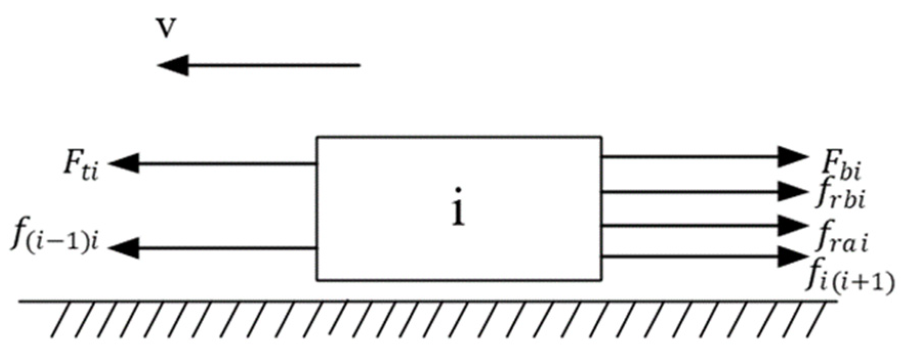
2.3. Forces between Maglev Train Sections

According to force models between the multi-mass carriages of high-speed trains presented in the literature [17], it can be applied to maglev trains, where each section of the maglev train can be regarded as an independent mass, and the sections are connected with elastic and damping devices, as shown in Figure 2.

The coupling forces between the maglev train sections are as follows:

$$f_{i(i+1)}=k(x_i-x_{i+1})+d({\dot{x}}_i-{\dot{x}}_{i+1})$$

(11)

In the formula, $f_{i(i+1)}$ is the coupling force between $i$ and $i+1$ carriages, $k$ is the elasticity factor $(\mathrm{N}/\mathrm{m})$, $d$ is the damping factor $(\mathrm{N}\cdot \mathrm{s}/\mathrm{m})$, $x_i$, $x_{i+1}$ is the displacement, and ${\dot{x}}_i$, ${\dot{x}}_{i+1}$ is the speed.

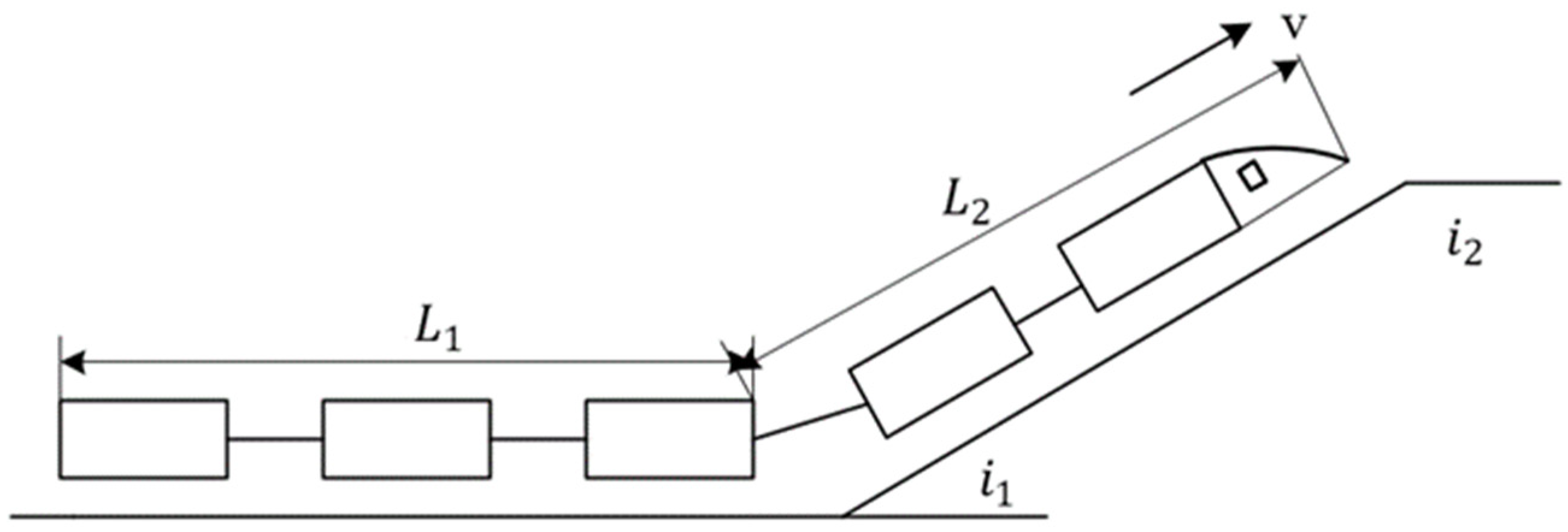
2.4. Multi-Mass Dynamics Model of Maglev Trains

One of the sections in the maglev train was selected for force analysis, as shown in Figure 3.

Based on multi-mass-point models of high-speed trains presented in the literature [18], electromagnetic drag, $f_e$, and linear generator operating drag, $f_d$, can be added and applied to a maglev train to elaborate a multi-mass-point dynamics and kinematics model for magnetic levitation trains.

In Figure 3, shows the traction force of section $i$, $F_{bi}$ shows the braking force of section $i$, $f_{rbi}$ shows the basic resistance of section $i$, $f_{rai}$ shows the additional resistance of section $i$, $f_{(i-1)i}$ shows the coupling force between section $i-1$ and section $i$, and $f_{i(i+1)}$ shows the coupling force between section $i$ and section $i+1$. $m_i$ is the mass of the carriage $i$, according to Newton’s second law of motion:

$$m_i{\ddot{x}}_i=F_{ti}-F_{bi}-f_{rbi}-f_{rai}+f_{(i-1)i}-f_{i(i+1)}$$

(12)

Carriage 1 can be expressed as carriage n by deriving it from Equation (12):

$$\left[\begin{array}{l}{m}_1{\ddot{x}}_1\\ m_2{\ddot{x}}_2\\ ...\\ m_n{\ddot{x}}_n\end{array}\right]=\left[\begin{array}{l}{F}_{t1}\\ F_{t2}\\ ...\\ F_{tn}\end{array}\right]-\left[\begin{array}{l}{F}_{b1}\\ F_{b2}\\ ...\\ F_{bn}\end{array}\right]-\left[\begin{array}{l}{f}_{rb1}\\ f_{rb2}\\ ...\\ f_{rbn}\end{array}\right]-\left[\begin{array}{l}{f}_{ra1}\\ f_{ra2}\\ ...\\ f_{ran}\end{array}\right]+\left[\begin{array}{c}{f}_{01}-f_{12}\\ f_{12}-f_{23}\\ ...\\ f_{(n-1)n}-f_{n(n+1)}\end{array}\right]$$

(13)

Then, substituting Equation (11) into the last term in Equation (13) gives:

$$\left[\begin{array}{c}{f}_{01}-f_{12}\\ f_{12}-f_{23}\\ ...\\ f_{(n-2)(n-1)}-f_{(n-1)n}\\ f_{(n-1)n}-f_{n(n+1)}\end{array}\right]$$

(14)

The first section is only subject to coupling force from the back section, and the last section is only subject to coupling force from the front section; therefore, $f_{01}=0$, $f_{n(n+1)}=0$.

$$\left[\begin{array}{c}0\\ k(x_1-x_2)+d({\dot{x}}_1-{\dot{x}}_2)\\ ...\\ k(x_{n-2}-x_{n-1})+d({\dot{x}}_{n-2}-{\dot{x}}_{n-1})\\ k(x_{n-1}-x_n)+d({\dot{x}}_{n-1}-{\dot{x}}_n)\end{array}\right]-\left[\begin{array}{c}k(x_1-x_2)+d({\dot{x}}_1-{\dot{x}}_2)\\ k(x_2-x_3)+d({\dot{x}}_2-{\dot{x}}_3)\\ ...\\ k(x_{n-1}-x_n)+d({\dot{x}}_{n-1}-{\dot{x}}_n)\\ 0\end{array}\right]$$

(15)

Adding the two sides of Equation (13), in turn, it is clear from Equation (15) that the coupling forces between the sections of the maglev train cancel out, giving:

$$m_1{\ddot{x}}_1+m_2{\ddot{x}}_2+...+m_n{\ddot{x}}_n={\displaystyle \sum _{i=1}^n{F}_{ti}}-{\displaystyle \sum _{i=1}^n{F}_{bi}}-{\displaystyle \sum _{i=1}^n{f}_{rbi}}-{\displaystyle \sum _{i=1}^n{f}_{rai}}$$

(16)

Notably, $\Delta x_{i-1}$ denotes the difference in displacement obtained between the adjacent $i$ and $i-1$ compartments. ${\ddot{x}}_i$, ${\ddot{x}}_{i-1}$ is the acceleration of the section, and $\Delta {\ddot{x}}_{i-1}$ is the relative acceleration between sections.

$$x_i-x_{i-1}=\Delta x_{i-1}$$

(17)

$${\ddot{x}}_i-{\ddot{x}}_{i-1}=\Delta {\ddot{x}}_{i-1}$$

(18)

Choosing the first maglev train section as the reference point, the acceleration relationship between the first section and section $i$ is given by Equation (18).

$${\ddot{x}}_i={\ddot{x}}_1+{\displaystyle \sum _{k=1}^{i-1}\Delta {\ddot{x}}_k}$$

(19)

where:

$$\left[\begin{array}{l}{m}_1{\ddot{x}}_1\\ m_2{\ddot{x}}_2\\ m_3{\ddot{x}}_3\\ ...\\ m_n{\ddot{x}}_n\end{array}\right]=\left[\begin{array}{l}{m}_1{\ddot{x}}_1\\ m_2({\ddot{x}}_1+\Delta {\ddot{x}}_1)\\ m_3({\ddot{x}}_1+\Delta {\ddot{x}}_1+\Delta {\ddot{x}}_2)\\ ...\\ m_n({\ddot{x}}_1+\Delta {\ddot{x}}_1+...+\Delta {\ddot{x}}_{n-1})\end{array}\right]$$

(20)

$${\displaystyle \sum _{i=1}^n{F}_{ti}-}{\displaystyle \sum _{i=1}^n{F}_{bi}-}{\displaystyle \sum _{i=1}^n{f}_{rbi}-}{\displaystyle \sum _{i=1}^n{f}_{rai}=\lambda (t)}$$

(21)

Substituting Equation (20) for Equation (16), the multi-mass dynamics and kinematics model of the maglev train is as follows:

$${\ddot{x}}_1{\displaystyle \sum _{i=1}^n{m}_i=\lambda (t)-\Delta {\ddot{x}}_1}{\displaystyle \sum _{i=2}^n{m}_i-}\Delta {\ddot{x}}_2{\displaystyle \sum _{i=3}^n{m}_i-}...-\Delta {\ddot{x}}_{n-1}{m}_n$$

(22)

The multi-mass-point dynamics and kinematics model of the maglev train takes into account the electromagnetic resistance and linear generator running resistance of the maglev train, as well as the coupling forces between the carriages; it also considers the special working conditions of slopes, curves and tunnels, which describe the actual operation of maglev trains more accurately than the single-mass-point model of maglev trains.

3. Radial-Based Neural Network for the Displacement-Limited Operation Control of Maglev Trains

To ensure the safe operation of a maglev train system and that the overshoot cannot impact the safety of the system, the upper and lower bounds of the position and speed signals of the maglev train system need to be strictly limited, and the maglev train will be limited in two aspects during operation, namely, output-limited and state-limited. $u_{\max }(t)$ and $u_{\min }(t)$ denote the input upper and lower bounds of the system control during operation of the maglev train, respectively. $k$ denotes the system order of the maglev train operation process, $k=1,2$; $x_{k,\max }(t)$ and $x_{k,\min }(t)$ are the upper and lower bounds of the system state signal during the operation of maglev trains. The output limit can be expressed as [19]:

$$u_{\min }(t)\le u_i(t)\le u_{\max }(t)$$

(23)

$$x_{k,\min }(t)\le x_{k,i}(t)\le x_{k,\max }(t)$$

(24)

The objective of this study was to develop a radial-based neural-network-based control system to accurately track the target desired curve within a constrained range for a given desired position profile, $x_d$, and desired speed profile, $y_d$, during the operation of a maglev train, subject to output constraints and state constraints.

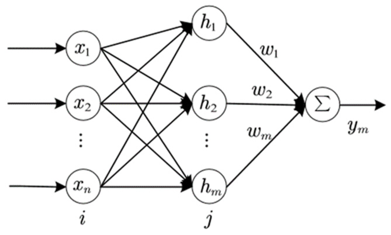
3.1. Radial-Based Neural Network

The radial-based neural network structure was selected because of the strong real-time nature of maglev trains during operation. This neural network structure is characterized by nonlinear mapping from the input layer to the output layer, and a linear relationship between the output layer and the adjustable parameters, which has an advantage; the weight values of the neural network can be solved by linear equations without the need for extensive error estimations to adjust each node of each layer of the neural network. This is in line with the real-time control of maglev train operating state processes, avoiding the problem of a local minimum [20,21,22] and speeding up the learning rate in real time. The structure of the radial-based neural network is shown in Figure 4.

The network inputs the initial values of the position and speed of the maglev train: $x={\left[x_1{x}_2\right]}^T$. The neuron activation function of the hidden layer of the neural network consists of a radial-based function, and the array of arithmetic units, comprising the hidden layer, are called the hidden layer nodes. The hidden layer output of the neural network is $h={[h_j]}^T$, where $h$ represents the displacement limit of a magnetic levitation train, and the output expression of the implicit layer [23] is:

$$h_j=\exp (-\frac{{\Vert x-c_{ij}\Vert }^2}{2b_j^2})$$

(25)

where $c_{ij}$ is the coordinate vector of the centroid of the Gaussian basis function of the $j$ neuron node. $b_j$ is the width of the basic function of the $j$ neuron node in the hidden layer, $w$ is the weight of the radial-based neural network, and $i=1,2,...,n$; $j=1,2,...,m.$ The radial-based neural network output can be expressed as:

$$c=[c_{ij}]=\left[\begin{array}{ccc}{c}_{11}& ...& c_{1m}\\ ...& ...& ...\\ c_{n1}& ...& c_{nm}\end{array}\right]$$

(26)

$$b={[b_1,...,b_m]}^T$$

(27)

$$w={[w_1,...,w_m]}^T$$

(28)

$$y(t)=w^{T}h=w_1{h}_1+w_2{h}_2+...+w_m{h}_m$$

(29)

3.2. Radial-Based Neural Network for the Design of a Displacement-Constrained Operation Controller for Maglev Trains

This study presents the first application of an RBF neural network in the displacement-constrained control of maglev trains and constructs weights using the stability theory. The innovative aspect is that the value of the position signal and the command signal after subtraction can be guaranteed to be less than the given safety limit at any moment when the time is greater than zero. The safety constraint on the displacement and speed of the maglev train ensures stability and safety during its operation.

Based on the maglev train dynamics model, it can be transformed into the system state-space equation:

$$\{\begin{array}{l}{\dot{x}}_1=x_2\\ {\dot{x}}_2=f(t)+bu\end{array}$$

(30)

$$f(t)=\lambda (t)/{\displaystyle \sum _{i=1}^n{m}_i}$$

(31)

where $x_1$ is the maglev train displacement signal, $x_2$ is the speed signal of the maglev train, and $f(t)$ is the time-varying state variable of the maglev train. By designing control laws to achieve $\forall t\ge 0$ and $t\to \infty$, $x_1\to y_d$, $x_2\to {\dot{y}}_d$, and $\left|x_1(t)\right|<k_c$. $y_d$ is a displacement signal command; ${\dot{y}}_d$ is a speed signal command. $k_c$ is the limit value of the position signal.

Displacement signal error:

$$z_1=x_1-y_d$$

(32)

We let $\left|z_1(t)\right|<k_b$ to obtain $-k_b+y_{d\min }<x_1<k_b+y_{d\max }$. The problem can be translated into the design of the control law to achieve $\forall t\ge 0$,$\left|z_1(t)\right|<k_b$. $k_b$ is the limit value for subtracting the position signal from the command signal. According to Equation (32), we can derive ${\dot{z}}_1=x_2-{\dot{y}}_d$ and define $z_2=x_2-\alpha$ [15]; $\alpha$ is the stability function to be designed. Then, the following Lyapunov function can be defined [24,25]:

$$V_1=\frac{1}{2}\ln \frac{k_b^2}{k_b^2-z_1^2}$$

(33)

$${\dot{V}}_1=\frac{z_1{\dot{z}}_1}{k_b^2-z_1^2}=\frac{z_1(z_2+\alpha -{\dot{y}}_d)}{k_b^2-z_1^2}$$

According to the above form, the stability function can be designed as $\alpha =-k_1{z}_1+{\dot{y}}_d$, $k_1>0$.

${\dot{V}}_1=-\frac{k_1{z}_1^2}{k_b^2-z_1^2}+\frac{z_1{z}_2}{k_b^2-z_1^2}$ When $z_2=0$, ${\dot{V}}_1\le 0$, the Lyapunov function can be re-defined:

$$V_2=V_1+\frac{1}{2}{z}_2^2$$

(34)

$${\dot{z}}_2={\dot{x}}_2-\dot{\alpha }=f(t)+bu-\dot{\alpha }$$

therefore:

$${\dot{V}}_2={\dot{V}}_1+z_2{\dot{z}}_2=-\frac{k_1{z}_1^2}{k_b^2-z_1^2}+\frac{z_1{z}_2}{k_b^2-z_1^2}+z_2[f(t)+bu-\dot{\alpha }]$$

The Lyapunov function can be designed as [24]:

$$V=V_2+\frac{1}{2\gamma }{\tilde{W}}^T\tilde{W}=\frac{1}{2}\log \frac{k_b^2}{k_b^2-z_1^2}+\frac{1}{2}{z}_2^2+\frac{1}{2\gamma }{\tilde{W}}^T\tilde{W}$$

(35)

$$\tilde{W}=\widehat{W}-W^{*}$$

$\widehat{W}$ is the actual weight of the radial-based neural network, and $W^{*}$ is the ideal weight of the radial-based neural network. The ideal weight, $W^{*}$, is the ideal connection between neurons; an output is calculated after inputting the data, and then the error is back-propagated after comparing it with the actual output; the weights are continuously adjusted, and the new weights are generated to be adjusted again after comparing them with the ideal weights, $W^{*}$, until the ideal error is reached. The ideal weights $W^{*}$ are set before training, and the actual weights $\widehat{W}$ are obtained during training. The neural network keeps narrowing the difference between them in the training process, so that the actual weights gradually approach the ideal weights. The derivative of Equation (35) gives:

$$\dot{V}=-\frac{k_1{z}_1^2}{k_b^2-z_1^2}+\frac{z_1{z}_2}{k_b^2-z_1^2}+z_2[f(t)+bu-\dot{\alpha }]+\frac{1}{\gamma }{\tilde{W}}^T\dot{\widehat{W}}$$

The control rate can be designed as:

$$u=\frac{1}{b}[-\widehat{f}(t)+\dot{\alpha }-k_2{z}_2-\frac{z_1}{k_b^2-z_1^2}](k_2>0)$$

(36)

$$\dot{V}=-\frac{k_1{z}_1^2}{k_b^2-z_1^2}-k_2{z}_2^2+z_2[f(t)-\widehat{f}(t)]+\frac{1}{\gamma }{\tilde{W}}^T\dot{\widehat{W}}$$

In radial-based neural networks, $f(t)$, $h$ is the output of the Gaussian basis function of the radial-based neural network, and $\epsilon$ is the approximation error value. When the network inputs the initial values of the maglev train displacement and speed signals, the output is $\widehat{f}(t)$; thus:

$$f(t)-\widehat{f}(t)=W^{*T}h(t)+\epsilon -{\widehat{W}}^{T}h(t)=-{\tilde{W}}^{T}h(t)+\epsilon$$

$$\dot{V}=-\frac{k_1{z}_1^2}{k_b^2-z_1^2}-k_2{z}_2^2+z_2[-{\tilde{W}}^{T}h(t)+\epsilon ]+\frac{1}{\gamma }{\tilde{W}}^T\dot{\dot{\widehat{W}}}$$

$$=-\frac{k_1{z}_1^2}{k_b^2-z_1^2}-k_2{z}_2^2+{\tilde{W}}^T[\frac{1}{\gamma }\dot{\widehat{W}}-z_{2}h(t)]+\epsilon z_2$$

The adaptive rate can be set as:

$$\dot{\widehat{W}}=\gamma z_{2}h(t)-\gamma \widehat{W}$$

$$\dot{V}=-\frac{k_1{z}_1^2}{k_b^2-z_1^2}-k_2{z}_2^2-{\tilde{W}}^T\widehat{W}+\epsilon z_2$$

$${\tilde{W}}^T\widehat{W}={\tilde{W}}^T(\tilde{W}+W^{*})={\tilde{W}}^T\tilde{W}+{\tilde{W}}^T{W}^{*}$$

$$=\frac{3}{4}{\tilde{W}}^T\tilde{W}+\frac{1}{4}{\tilde{W}}^T\tilde{W}+{\tilde{W}}^T{W}^{*}\ge \frac{3}{4}{\tilde{W}}^T\tilde{W}-W^{*T}{W}^{*}$$

$$-{\tilde{W}}^T\widehat{W}\le -\frac{3}{4}{\tilde{W}}^T\tilde{W}+{\Vert W^{*}\Vert }^2$$

According to the prior analyses [26], this satisfies $\forall t\ge 0$, $\left|z_1(t)\right|<k_b$. When $\forall t\in [0,\infty )$, $\ln \frac{k_b^2}{k_b^2-z_1^2}<\frac{z_1^2}{k_b^2-z_1^2}$. Additionally, $\epsilon z_2\le \frac{1}{4}{\epsilon }^2+z_2^2$.

$$\dot{V}\le -k_1\ln \frac{k_b^2}{k_b^2-z_1^2}-k_2{z}_2^2-\frac{3}{4}{\tilde{W}}^T\tilde{W}+{\Vert W^{*}\Vert }^2+\frac{1}{4}{\epsilon }^2+z_2^2$$

We let [26]:

$$\xi ={\Vert W^{*}\Vert }^2+\frac{1}{4}{\epsilon }^2$$

$$\eta =\min [2k_1,2(k_2-1),\frac{3}{2}\gamma ]$$

then:

$$\dot{V}\le \xi -\eta V$$

According to [26], we can determine that $V$ is bounded; thus, $z_1$, $z_2$ and $\tilde{W}$ are also bounded. In the case of satisfying $\forall t\ge 0$, $\left|z_1(t)\right|<k_b$. $V(t)\le e^{-\eta t}V(0)+\frac{\xi }{\eta }(1-e^{-\eta t})$, $t\to \infty$ and $V(t)\to \frac{\xi }{\eta }$ gradually converge to make it bounded. This shows that the method can make the system stable, when $\xi \ll \eta$, $V(t)\to 0$, $z_1$, $z_2\to 0$, i.e., the maglev train displacement signal $x_1$ converges to the displacement signal command $y_d$, and the maglev train speed signal $x_2$ converges to the speed signal command ${\dot{y}}_d$. It is possible to keep the maglev train displacement and speed values within the constraint limits.

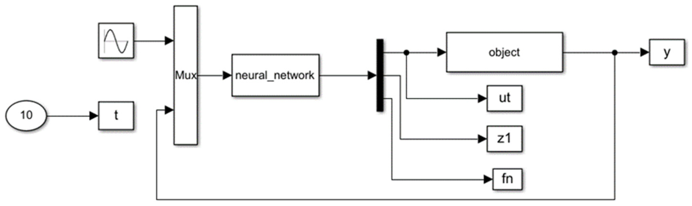
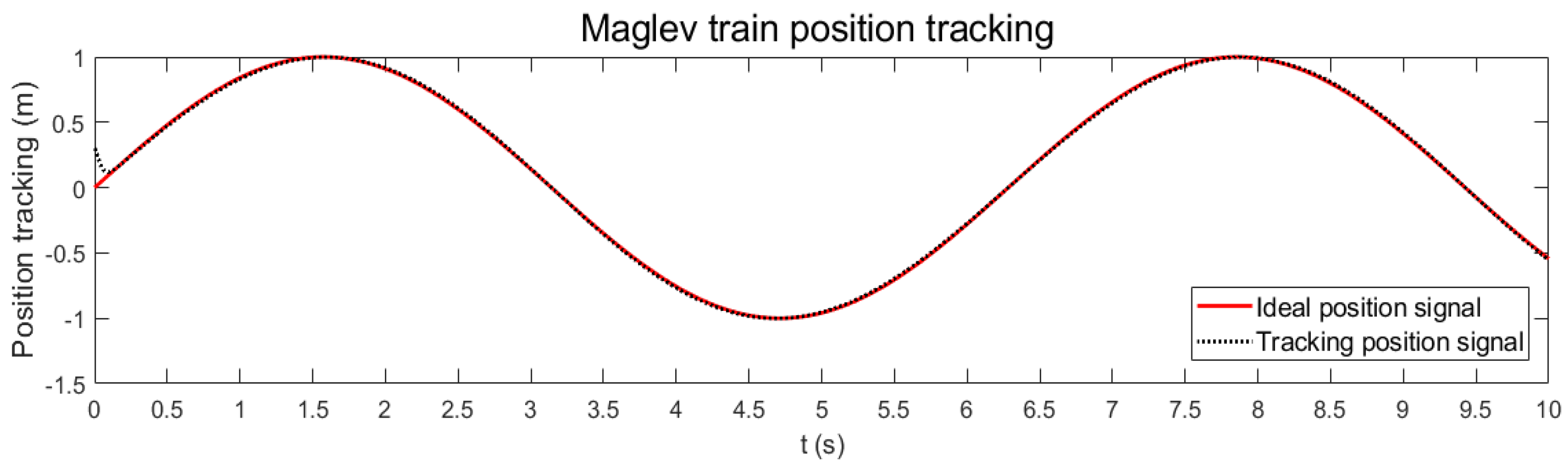
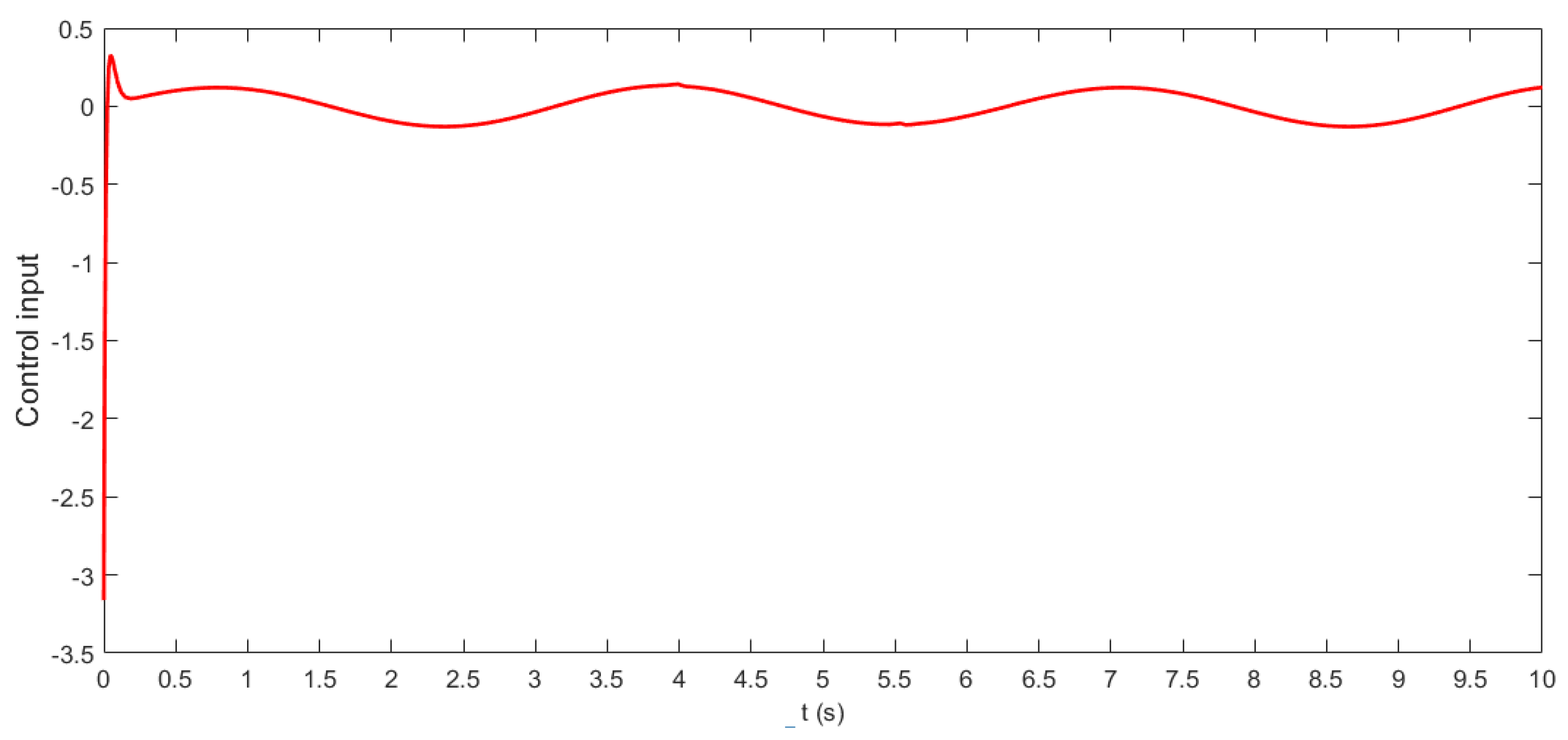
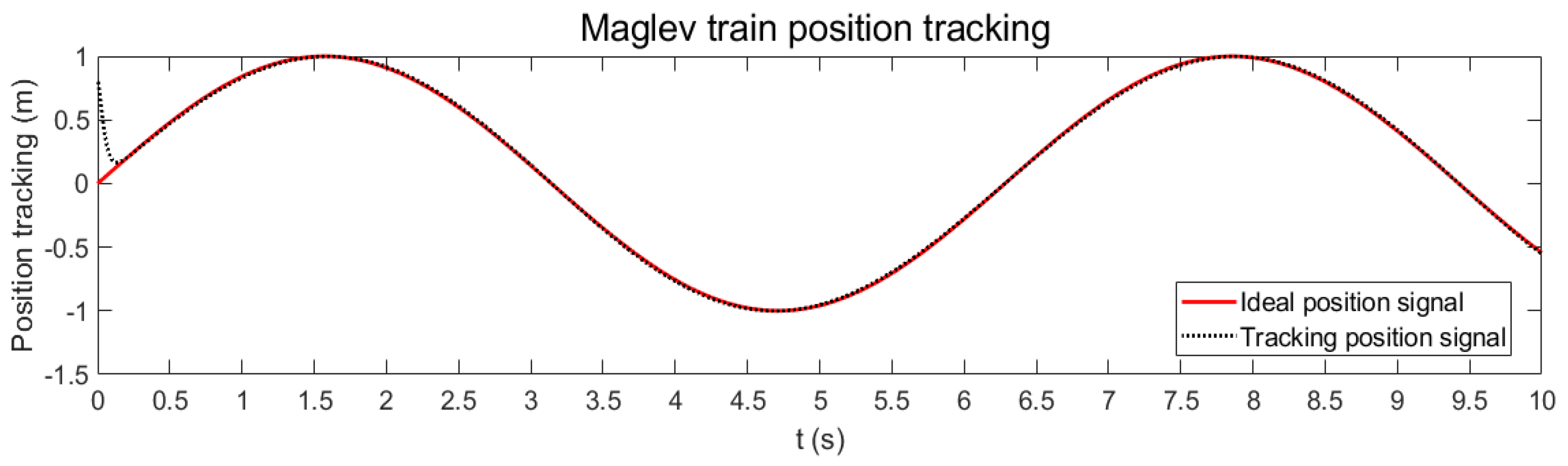
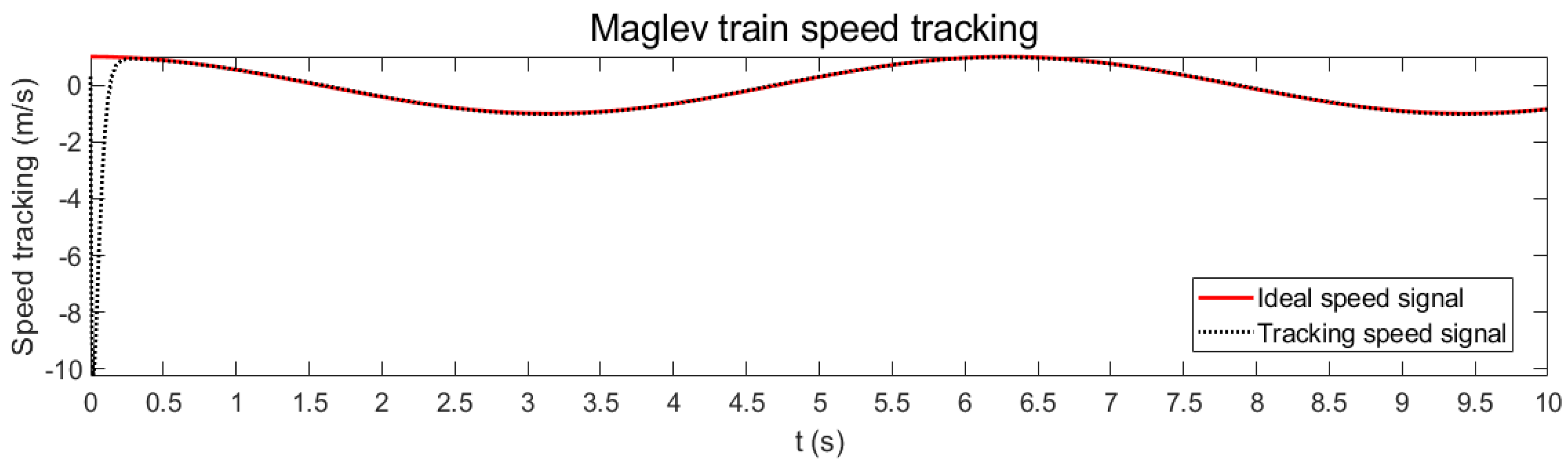
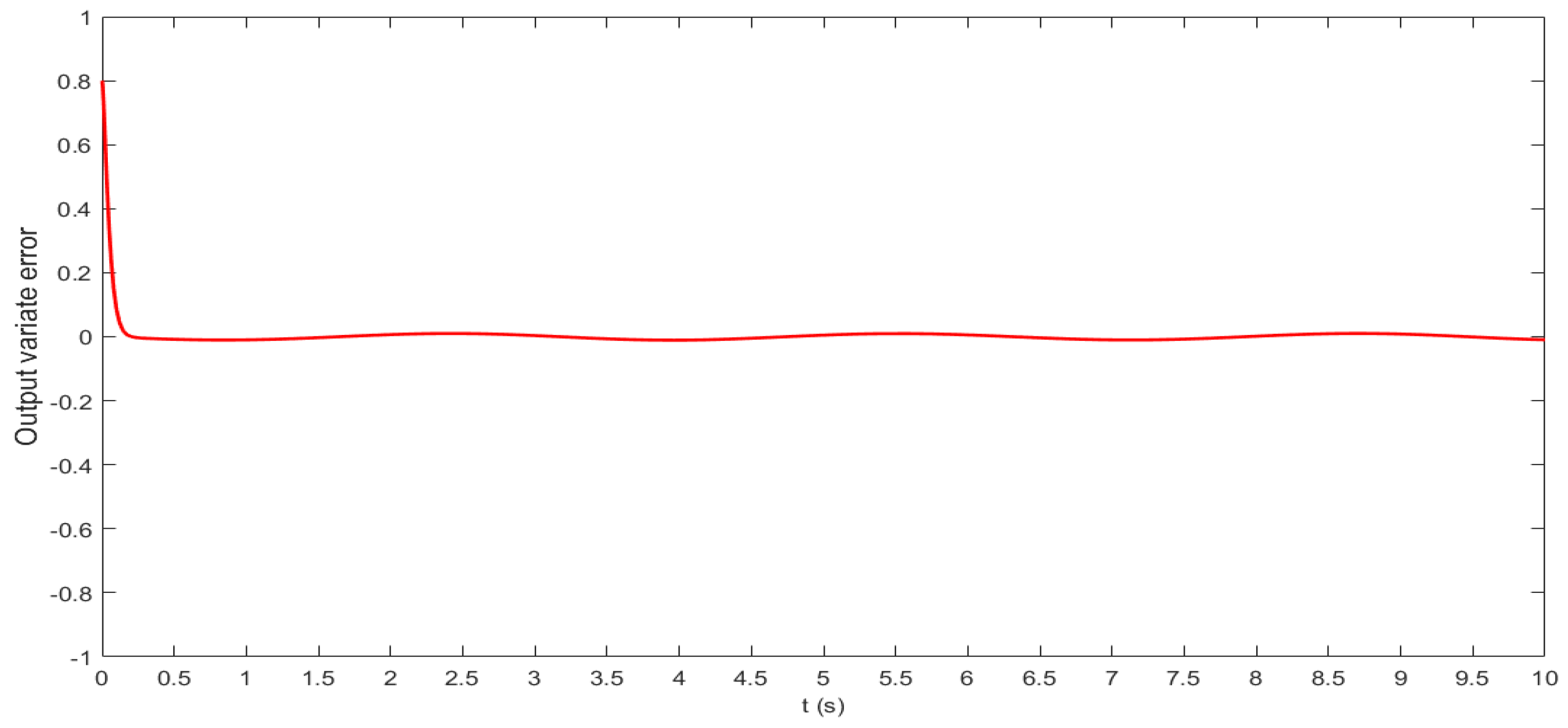
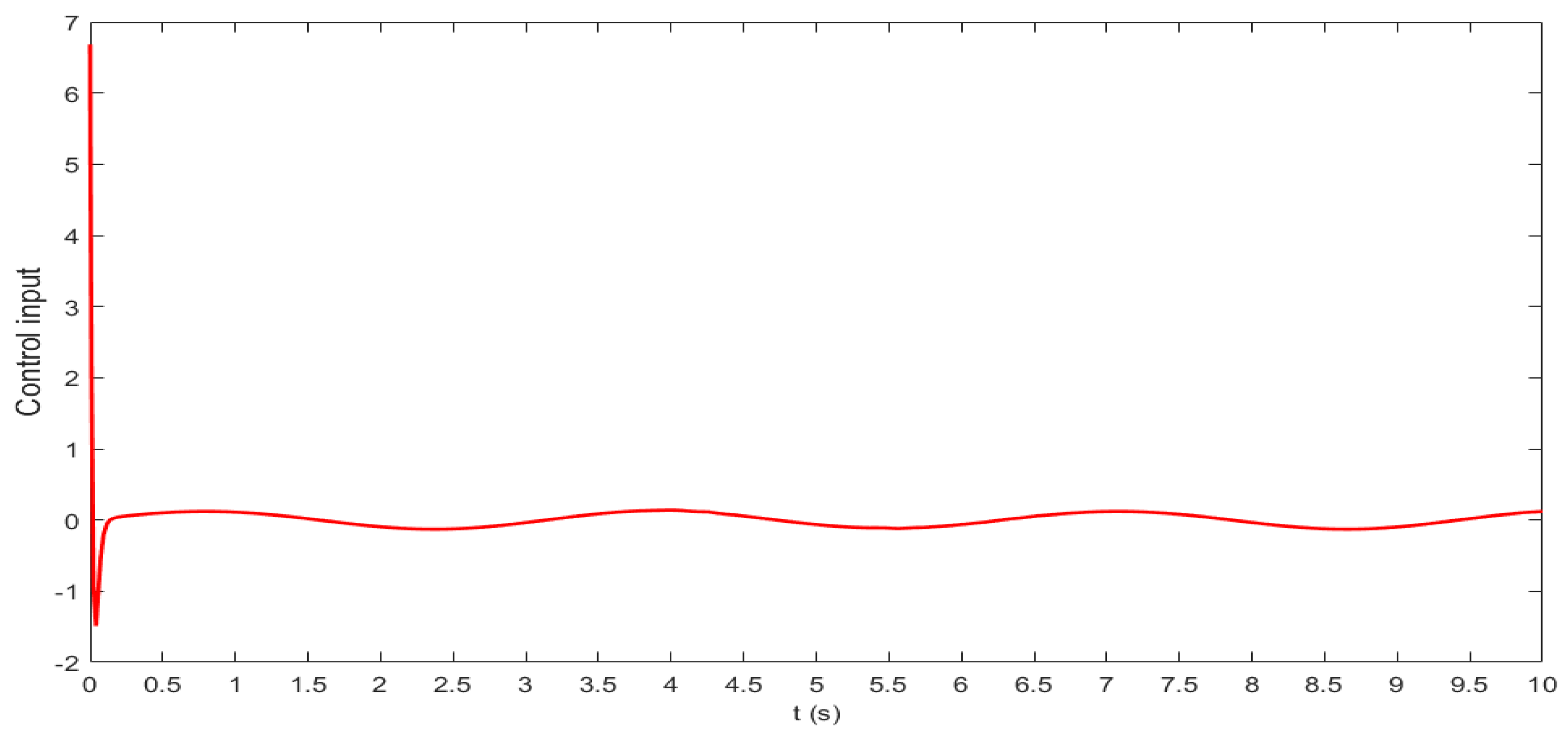
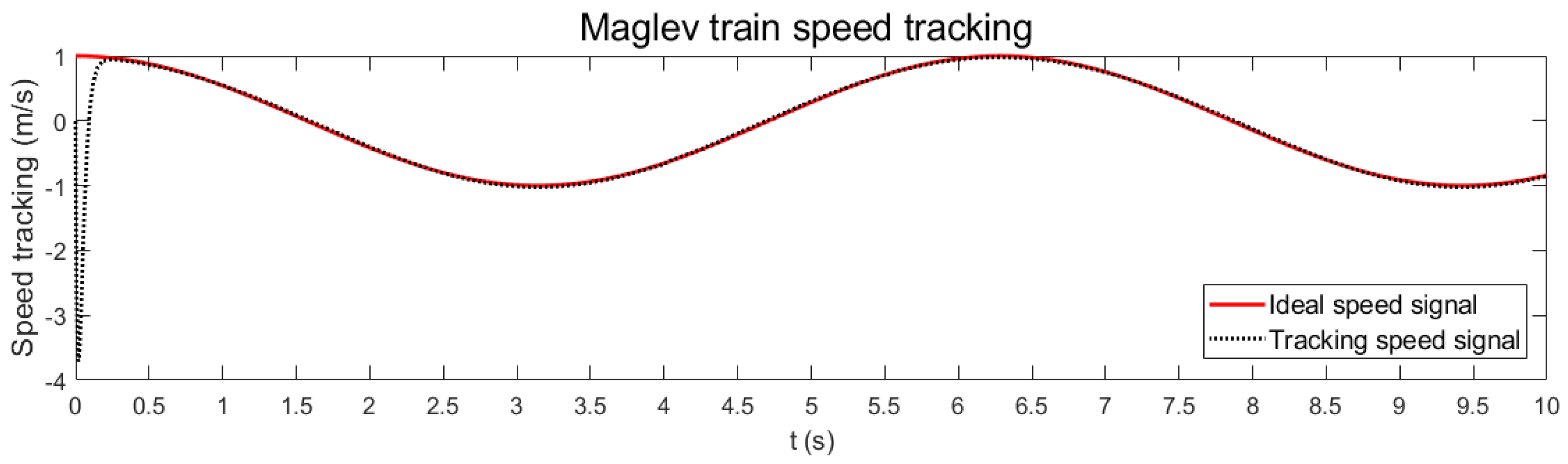
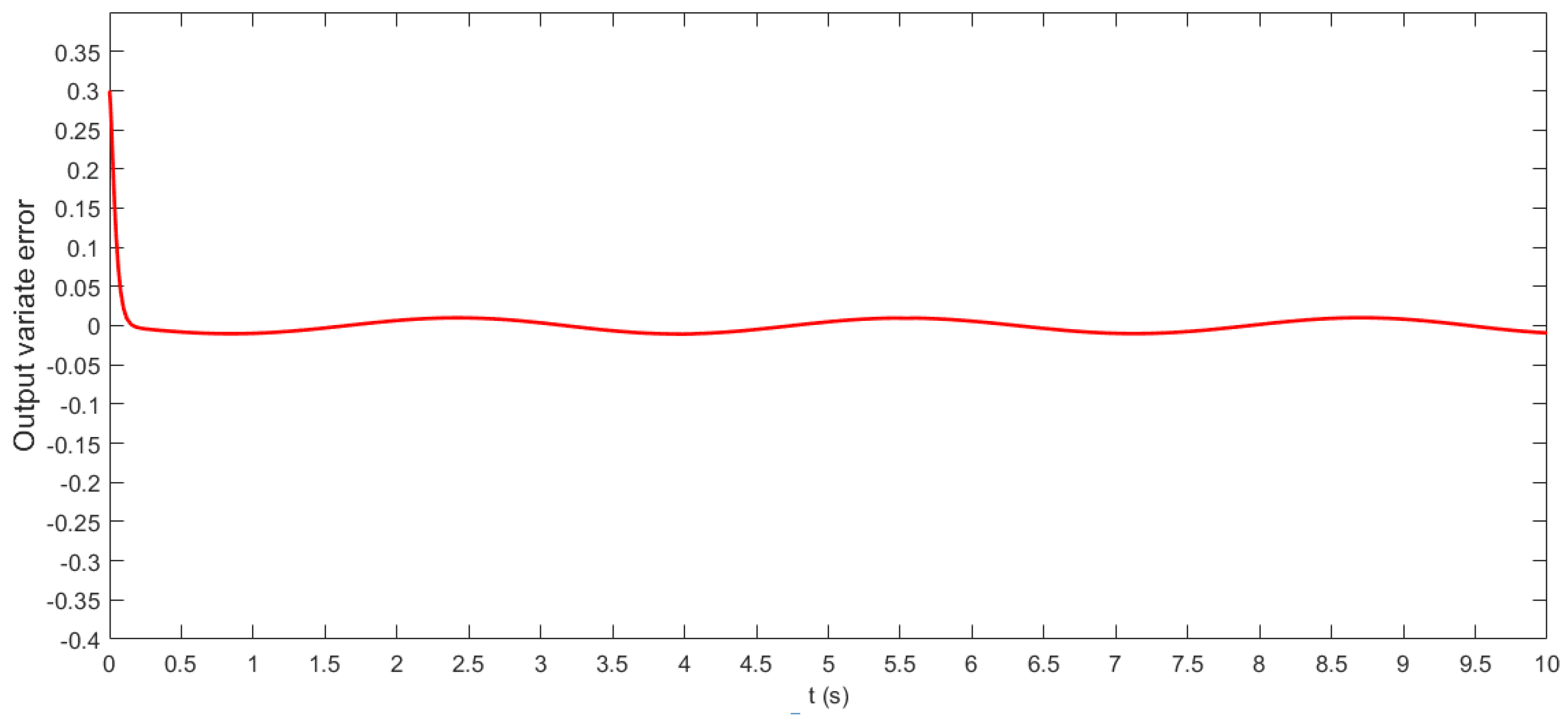
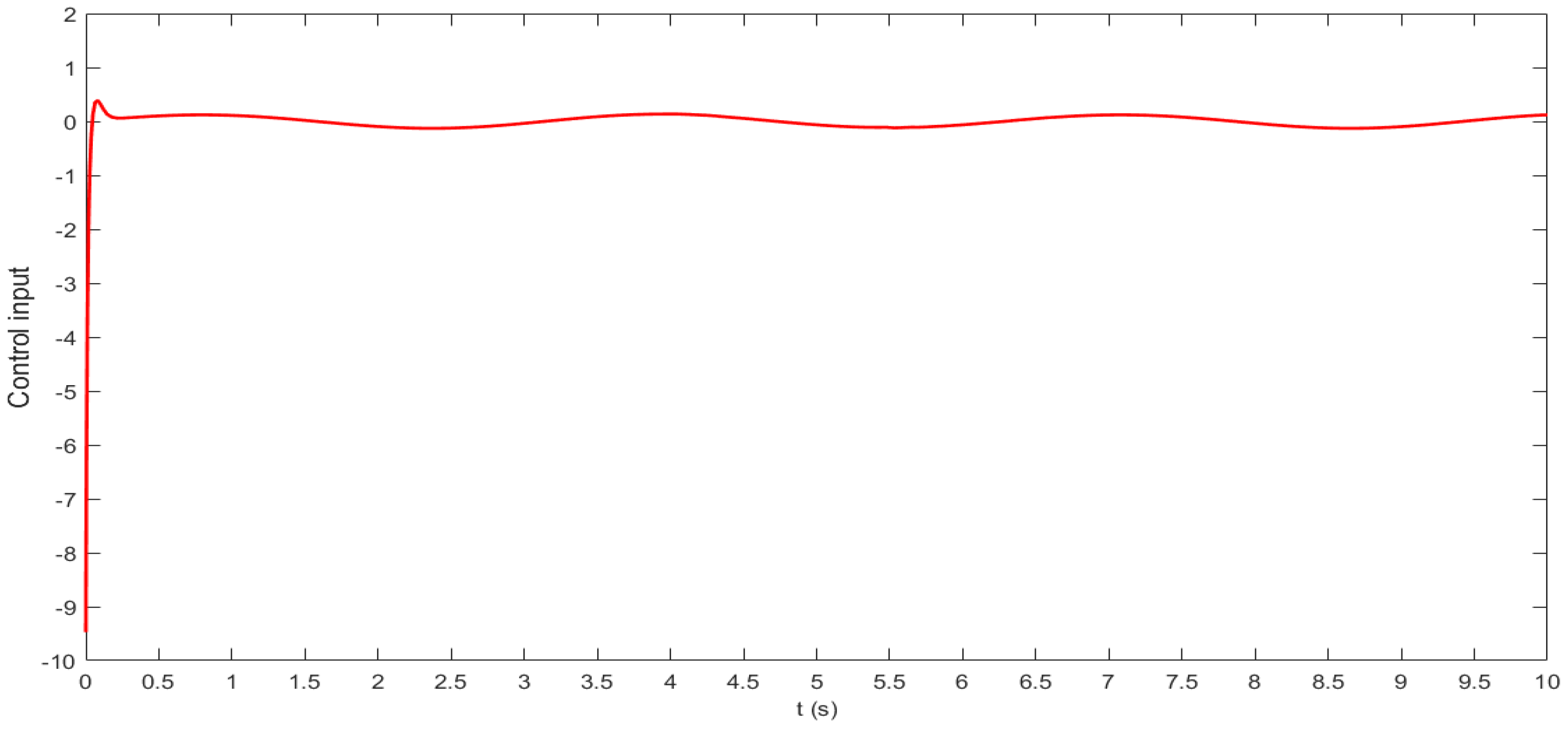
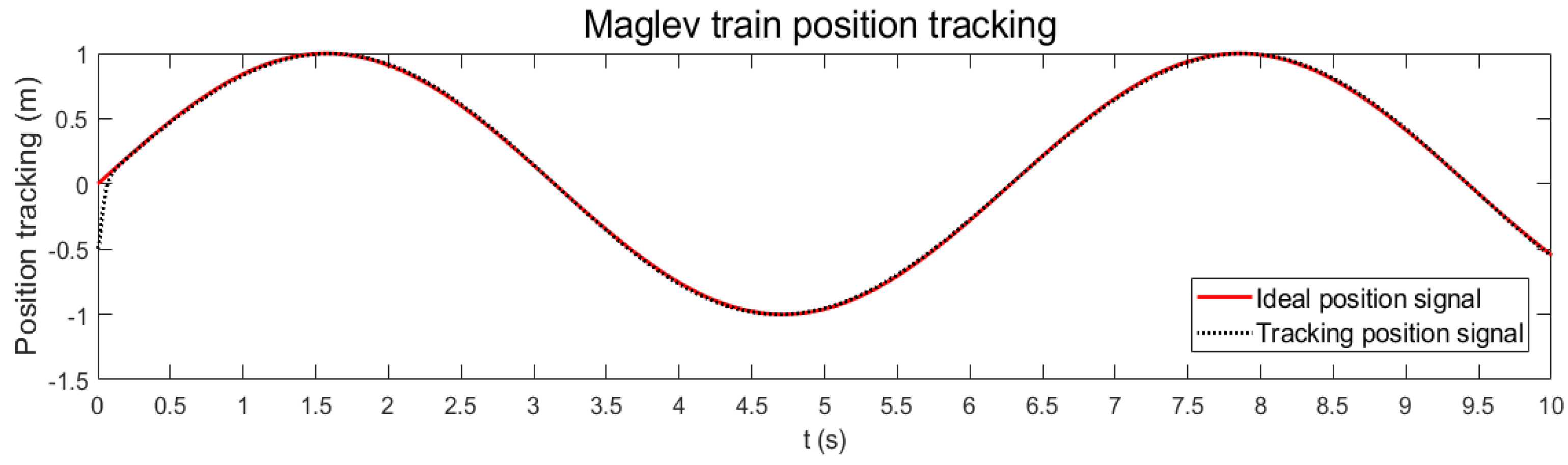
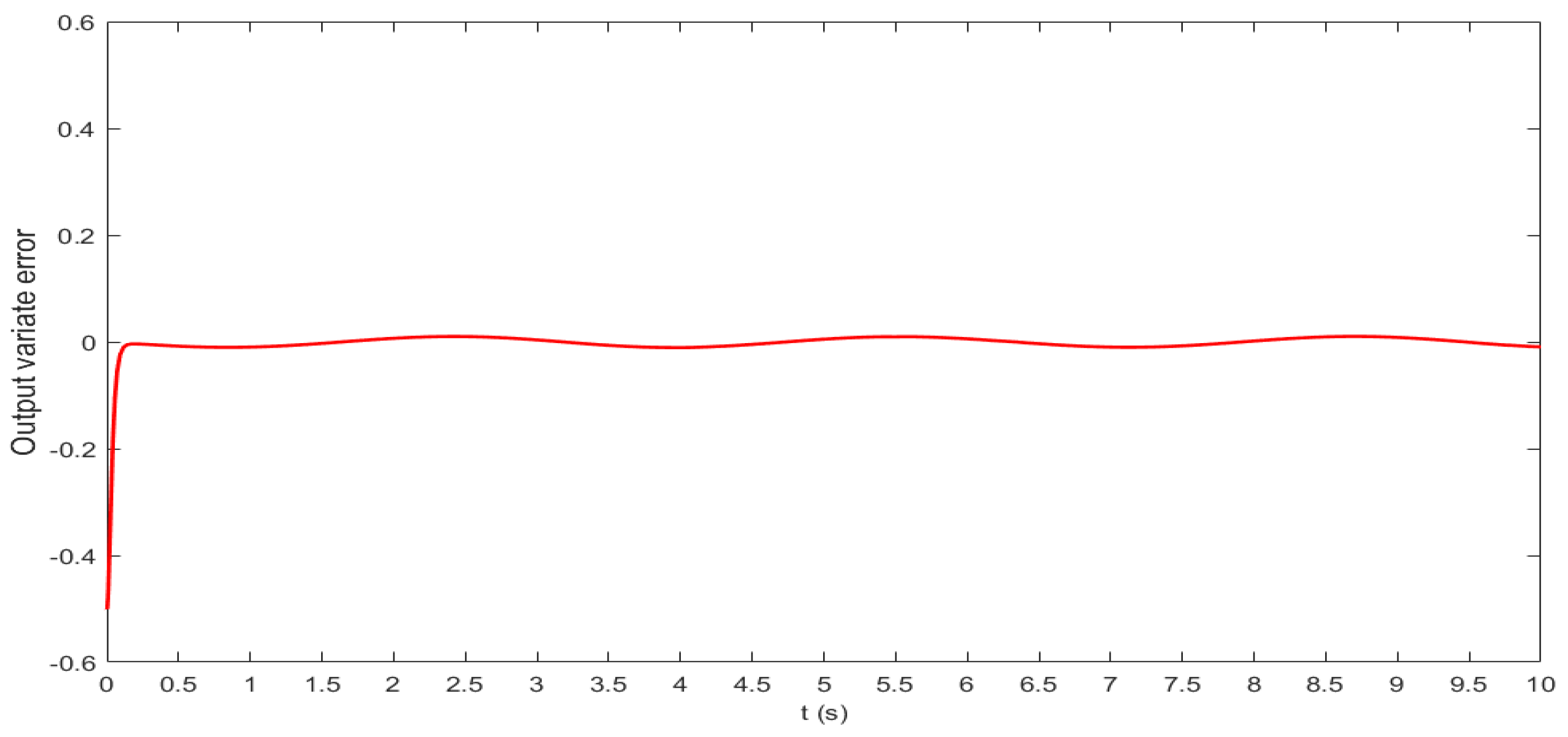
3.3. System Simulation

In this study, a multi-mass-point model was used in the dynamic modeling process of maglev trains, and the initial state input of the controlled object was $[0.30]$. Specifically, the initial value of displacement was $0.3\mathrm{m}$, and the initial value of velocity was $0\mathrm{m}/\mathrm{s}$; it was determined that $f(t)=-43x_1{x}_2$ and $b=172$. Traction, speed uniformity and braking are all aspects of maglev train operation. In this paper, we chose the displacement signal command $y_d=\sin t$ at the initial moment of $t=0$. $z_1=x_1-y_d=0.3$; at this time, the value $k_b=0.31$ was taken. The maglev train displacement signal $x_1$ was limited to $\pm 1.31$, and the constant was taken as $\frac{1}{2\gamma }=5$, $k_1=k_2=46$. In radial-based neural networks, the Gaussian basis function parameter $c_i$ is the coordinate vector of the center point of the Gaussian basis function, the value of $c_i$ is closer to the input value, and the Gaussian basis function is more sensitive to the input; here, $c_i$ can be taken as $\left[-1-0.500.51\right]$. The value of $b_i$ is the width of the Gaussian basis function; the larger the value, the wider the function, and the greater the mapping ability of the radial-based neural network. When setting $b_i$ to a suitable value, i.e., $b_i=1.5$, in radial-based neural networks, each initial weight value can be taken as $0.2$. Figure 5 shows a simulation model of speed and displacement in limited operation control of a maglev train. Figure 6 shows the ideal displacement signal curve and tracking position signal curve of a maglev train. Figure 7 shows the ideal speed signal curve and tracking speed signal curve of a maglev train. Figure 8 shows that the control input values are large in absolute value before $0.2\mathrm{s}$, and then gradually converge to stability. Figure 9 shows that the subsequent error can be kept within the stable range.

In order to verify the validity and stability of the model under different input operating conditions, the initial state input of the controlled object was changed to $\left[0.80.3\right]$, i.e., the initial value of displacement was $0.8\mathrm{m}$, and the initial value of velocity was $0.3\mathrm{m}/\mathrm{s}$. $f(t)=-43x_1{x}_2$ and $b=172$ were set; traction, homogeneous speed and braking are all key aspects of maglev trains throughout the operation process. The displacement signal command $y_d=\sin t$ can be selected at the initial moment of $t=0$, $z_1=x_1-y_d=0.8$, when it takes a value of $k_b=0.81$. The magnetic levitation train displacement signal $x_1$ is constrained at approximately $\pm 1.81$; the constants are taken as $\frac{1}{2\gamma }=5$, $k_1=k_2=46$, and $c_i$ as $[-1-0.500.51]$, $b_i=1.5$; and the initial weight of each radial-based neural network is taken as $0.2$. Figure 10 shows the ideal displacement signal curve and tracking position signal curve of a maglev train. Figure 11 shows the ideal speed signal curve and tracking speed signal curve of a maglev train. Figure 12 shows that the control input values are large in absolute value before $0.2\mathrm{s}$, and then gradually converge to stability. Figure 13 shows that the subsequent error can be kept within the stable range.

The initial state input of the controlled object can be changed to $\left[-0.50\right]$, i.e., the initial value of displacement is $-0.5\mathrm{m}$, and the initial value of speed is $0\mathrm{m}/\mathrm{s}$, setting $f(t)=-43x_1{x}_2$, $b=172$; traction, uniformity and braking are all associated with maglev train operation. The displacement signal command $y_d=\sin t$ is chosen for the initial moment in $t=0$, $z_1=x_1-y_d=-0.5$, at which point it is taken as $k_b=-0.51$, and the maglev train displacement signal $x_1$ is constrained at approximately $\pm 1.51$, with constants taken as $\frac{1}{2\gamma }=5$, $k_1=k_2=46$ taken as $c_i$ for $[-1-0.500.51]$, $b_i=1.5$, and radial-based neural networks with each initial weight taken as $0.2$. Figure 14 shows the ideal displacement signal curve and tracking position signal curve of a maglev train. Figure 15 shows the ideal speed signal curve and tracking speed signal curve of a maglev train. Figure 16 shows that the control input values are large in absolute value before $0.2\mathrm{s}$, and then gradually converge to stability. Figure 17 shows that the subsequent error can be kept within the stable range.

Figures of displacement and velocity tracking curves show that the radial-based neural network multi-mass-point magnetic levitation train displacement-constrained operation controller design can ensure that the magnetic levitation train displacement and speed signals converge to the command signal and reach the target convergence position quickly—in around $0.2\mathrm{s}$. From Figures of control input curve, it can be seen that the control input values are large in absolute value before $0.2\mathrm{s}$, and then gradually converge to stability; from Figures of Output error curve, it can be seen that the subsequent error can be kept within the stable range; Simulation results show that the system effectiveness and stability are good under different operating conditions, and the control is rapid and accurate, which can limit the magnetic levitation train displacement and speed within the desired safety constraints.

4. Conclusions

In this study, a radial-based neural network was used to control the displacement limits of a magnetic levitation train based on a multi-mass-point model. Simulation experiments show that the method can make the displacement and velocity signals of the maglev train rapidly converge to the command signal, and the overshoot and error can be kept within the stable range; thus, the output of the displacement and velocity values of the maglev train can be strictly limited, and the displacement and velocity signals of the maglev train can be limited within the desired safety constraints. Moreover, the radial-based neural network structure accelerates the learning rate while avoiding the local minimum problem, which is consistent with ensuring the real-time control of maglev train operating state processes and can guarantee the operational stability and safety of maglev transportation systems.

References

1. Mao, Z.; Tao, G.; Jiang, B.; Yan, X.G. Adaptive Control Design and Evaluation for Multibody High-Speed Train Dynamic Models. IEEE Trans. Control. Syst. Technol. 2020, 29, 1061–1074. [Google Scholar] [CrossRef]
2. Wang, X.; Xiao, Z.; Chen, M.; Sun, P.; Wang, Q.; Feng, X. Energy-Efficient Speed Profile Optimization and Sliding Mode Speed Tracking for Metros. Energies 2020, 13, 6093. [Google Scholar] [CrossRef]
3. Liu, Y.; Fan, K.; Ouyang, Q. Intelligent Traction Control Method Based on Model Predictive Fuzzy PID Control and Online Optimization for Permanent Magnetic Maglev Trains. IEEE Access 2021, 9, 29032–29046. [Google Scholar] [CrossRef]
4. Pu, Q.; Zhu, X.; Zhang, R.; Liu, J.; Fu, G. Speed Profile Tracking by an Adaptive Controller for Subway Train Based on Neural Network and PID Algorithm. IEEE Trans. Veh. Technol. 2020, 69, 10656–10667. [Google Scholar] [CrossRef]
5. Jie, Y.; Jia, L.; Fu, Y.; Lu, S. Speed Tracking Based Energy-Efficient Freight Train Control Through Multi-Algorithms Combination. IEEE Intell. Transp. Syst. Mag. 2017, 9, 76–90. [Google Scholar]
6. Chou, M.; Xia, X.; Kayser, C. Modelling and model validation of heavy-haul trains equipped with electronically controlled pneumatic brake systems. Control Eng. Pract. 2007, 15, 501–509. [Google Scholar] [CrossRef]
7. Xu, J.; Du, Y.; Chen, Y.H.; Hong, G. Adaptive robust constrained state control for nonlinear maglev vehicle with guaranteed bounded airgap. IET Control Theory Appl. 2018, 12, 1573–1583. [Google Scholar] [CrossRef]
8. Sun, Y.; Xu, J.; Qiang, H.; Lin, G. Adaptive Neural-Fuzzy Robust Position Control Scheme for Maglev Train Systems with Experimental Verification. IEEE Trans. Ind. Electron. 2019, 66, 8589–8599. [Google Scholar] [CrossRef]
9. Yang, G. Research on Optimal Speed Profile and Tracking Control of High-Speed Maglev Trains. Ph.D. Thesis, Beijing Jiaotong University, Beijing, China, 2007. [Google Scholar]
10. Fan, C.; Wu, G.; Hu, G. Characterization of long-stator linear synchronous motors based on state equations. Micro Mot. (Servo Technol.) 2005, 38, 26–28. [Google Scholar] [CrossRef]
11. Lu, Q.; Chen, Y.; Ye, Y.; Fan, C. Calculation of reactance and force analysis of long-stator linear synchronous motors. Small Medium-Sized Mot. 2003, 3, 17–22. [Google Scholar]
12. Tsunashima, H.; Abe, M. Static and dynamic performance of permanent magnet suspension for maglev transport vehicle. Veh. Syst. Dyn. 1998, 29, 83–111. [Google Scholar] [CrossRef]
13. Cui, J. Calculation of Operating Speed Profile of Low and Medium Speed Maglev Trains. Master’s Thesis, Southwest Jiaotong University, Chengdu, China, 2012. [Google Scholar]
14. Jiang, Q.L.; Zhang, K.L.; Lian, C.S. Calculation of operating resistance of EMS-type maglev trains. Locomot. Electr. Transm. 1999, 10–12. [Google Scholar]
15. Guo, Y.Y. Research on Automatic Driving of High-Speed Trains Based on Fuzzy Predictive Control. Master’s Thesis, Lanzhou Jiaotong University, Lanzhou, China, 2020. [Google Scholar]
16. Hou, T.; Guo, Y.; Chen, Y.; Yang, H. Research on speed control of high-speed trains based on multi-mass point model. J. Railw. Sci. Eng. 2020, 2, 314–325. [Google Scholar]
17. Wang, L.S. Automatic Driving Predictive Control of High-Speed Trains Based on Multi-Mass Model. Ph.D. Thesis, Beijing Jiaotong University, Beijing, China, 2016. [Google Scholar]
18. Liang, X.R.; Xiao, L.; Wang, X.; Yang, S.W.; Dong, H.R. Design of a neural network PID controller for high-speed train speed tracking. Comput. Eng. Appl. 2021, 57, 7. [Google Scholar]
19. He, Z.-Y.; Yang, Z.-J.; Lu, J.-Y. Research on iterative learning control method for high-speed trains under constrained conditions. Railw. Stand. Des. 2019, 63, 7. [Google Scholar]
20. Chen, W.B.; Wu, X.B.; Pei, Y.R.; Li, J.A. Study on Adaptive PID Control Algorithm Based on RBF Neural Network. In Proceedings of the 3rd International Conference on Computational Intelligence and Industrial Application (PACIIA2010), Wuhan, China, 4–5 December 2010; pp. 341–344. [Google Scholar]
21. Wang, X.Y.; Zhang, Z.K. Research of RBF Neural Networks Algorithm to Fault Diagnosis of Rotary Machinery. In Proceedings of the IITA International Conference on Control, Automation and Systems Engineering, Zhangjiajie, China, 11–12 July 2009; pp. 331–334. [Google Scholar]
22. Chen, W.B.; Wu, X.B.; Pei, Y.R.; Li, J.A. Study on Adaptive PID Control Algorithm Based on RBF Neural Netwoik. In Proceedings of the International Conference on Intelligent Computation and Industrial Application (ICIA2011), Hong Kong, China, 18–19 June 2011; pp. 337–340. [Google Scholar]
23. Yue, C.; Song, J. Application of Combination Model Based on RBF Neural Network in GPS Elevation Fitting. J. Geomat. 2020, 45, 20–22. [Google Scholar] [CrossRef]
24. Liu, J.K. RBF Neural Network Adaptive Control MATLAB Simulation, 2nd ed.; Tsinghua University Press: Beijing, China, 2018. [Google Scholar]
25. Tee, K.P.; Ge, S.S.; Tay, E.H. Barrier Lyapunov Functions for the control of output-constrained nonlinear systems. Automatica 2009, 45, 918–927. [Google Scholar] [CrossRef]
26. Ren, B.; Ge, S.S.; Tee, K.P.; Lee, T.H. Adaptive Neural Control for Output Feedback Nonlinear Systems Using a Barrier Lyapunov Function. IEEE Trans. Neural Netw. 2010, 21, 1339–1345. [Google Scholar] [PubMed]
Figure 1. Schematic diagram of the ramp resistance of a multi-mass model maglev train.
Energies 15 03110 g001
Figure 2. Schematic diagram of the coupling of adjacent sections of a maglev train.
Energies 15 03110 g002
Figure 3. Force diagram of a single maglev train carriage.
Energies 15 03110 g003
Figure 4. Structure of radial-based neural network.
Energies 15 03110 g004
Figure 5. Simulation model.
Energies 15 03110 g005
Figure 6. Maglev train displacement tracking curve.
Energies 15 03110 g006
Figure 7. Speed tracking curve of a maglev train.
Energies 15 03110 g007
Figure 8. Control input curve.
Energies 15 03110 g008
Figure 9. Output error curve.
Energies 15 03110 g009
Figure 10. Maglev train displacement tracking curve.
Energies 15 03110 g010
Figure 11. Speed tracking curve of a maglev train.
Energies 15 03110 g011
Figure 12. Control input curve.
Energies 15 03110 g012
Figure 13. Output error curve.
Energies 15 03110 g013
Figure 14. Maglev train displacement tracking curve.
Energies 15 03110 g014
Figure 15. Speed tracking curve of a maglev train.
Energies 15 03110 g015
Figure 16. Control input curve.
Energies 15 03110 g016
Figure 17. Output error curve.
Energies 15 03110 g017
Publisher’s Note: MDPI stays neutral with regard to jurisdictional claims in published maps and institutional affiliations.