Article

Side Fins Performance in Biomimetic Unmanned Underwater Vehicle

Polish Naval Academy, Faculty of Mechanical and Electrical Engineering, Smidowicza 69, 81-127 Gdynia, Poland
Energies 2022, 15(16), 5783; https://doi.org/10.3390/en15165783
Submission received: 15 July 2022 / Revised: 1 August 2022 / Accepted: 7 August 2022 / Published: 9 August 2022
(This article belongs to the Special Issue Vehicles Dynamics and Propulsion Technologies)

Abstract

:
This paper presents the experimental research conducted for the Biomimetic Unmanned Underwater Vehicle (BUUV). The study’s major goal is to create a single, flexible side fin with adequate proportions and stiffness for an energy-efficient propulsion system. The experiments were carried out in a laboratory water tunnel equipped with a sensor for direct thrust measurement for various fin dimensions. Further, the particle image velocimetry (PIV) approach was used for a more in-depth examination of fluid–structure interaction (FSI) phenomena. The given experiments indicate the region of superior propulsion system performance and explain the main aspects that have influenced thrust generation using image processing and the PIV approach.

1. Introduction

Biomimetic propulsion systems used in underwater vehicles are based on biological species that evolved over time through natural selection [1,2]. Unlike screw-type propeller systems, biomimetic propeller systems move like a fish [3], a turtle [4], a seal [5], or other marine animal. By pushing the water against the passing wave, the undulatory action of the fins provides propulsion [6]. One of the most significant advantages of biomimetic propulsion systems is their reduced hydro-acoustic noise spectrum [7]. The energy efficiency of an undulating propulsion system is determined by a variety of construction and control parameters. For energy efficiency analysis, a diverse range of real fin shape species were digitised and analysed [8], ranging from homocercal tails with a low aspect ratio (square shape used by bluegill sunfish and rainbow trout) to high aspect ratio (lunate shape used by tuna and swordfish) and even the heterocercal caudal fin used by sharks. When cruising, high aspect ratio fins (tuna and shark) are more efficient (St < 0.4), whereas short aspect ratio caudal fins (catfish and trout) are more efficient when accelerating or manoeuvring (St > 0.4).
The underwater vehicles depicted in [9,10,11] have a hull produced by the coupling of rigid movable elements with a flexible fin at the end. This type of construction is difficult to control, costly, and increases the risk of electronic components flooding within. A cost is also significant when designing a BUUV swarm, as the expense rises dramatically. As a result, efforts are being made to develop a biomimetic propulsion system based on single, flexible fins. Two fins are mounted on both sides of the hull in this type of propulsion system, and two fins are implemented at the rear. Aside from thrust generation, the two side fins can control BUUV immersion, while the rear fins can control course. It is more convenient to stabilise the course using two tail fins [12], especially when considering the work condition for hydroacoustic sensors installed in BUUV [13,14,15].
The primary purpose of this research is to obtain a simpler structure propulsion system solution that is also more reliable and has a high energy efficiency. Instead of a multi-unit drive, the particular goal of the effort is to construct single fins with adequate size and stiffness that induces an oscillating movement in the water.
Images of BUUVs with two flexible tails and two flexible side fins are shown in Figure 1. The BUUV presented in Figure 1a,b is the next-generation BUUV built within the ambit of SABUVIS, a European Defense Agency project (category B), while the miniature version of the same vehicle is shown in Figure 1c. The miniature version of the vehicle was built for testing in a laboratory water tunnel to work on the propulsion system characteristics, particularly the construction and control algorithm for energy efficiency analysis and increasing drive performance [16].
The influence of tail oscillation on fluid flow around a hull creates vortices and necessitates thorough examination of the fluid–structure interaction (FSI) [17,18,19,20] and vortex structures [21]. The thrust and drag of fins are affected by their flexibility [22] and shape [23] for different fluid velocities [24], as well as different frequencies [25] and amplitudes of oscillation [26]. Because the shape of the hull generates turbulence in the area of effect of the tail fins, only the side fin parameters are studied in this study.
The LS-DYNA programme and incompressible computational fluid dynamics (ICFD) can be utilised for analysis, as shown in the paper [27], but only for a fin drag force in a BUUV. Despite the fact that the results were experimentally proven, the fin was analysed as a rigid body. Simulation models are also presented in publications such as [17,28] with determined fin or artificial fish shape as a function of time. However, this model does not take into account the interaction between the flexible fin and the fluid. The FSI analysis remains a difficult operation, and the findings are sensitive to parameter changes, even when using the smoothed particle hydrodynamics (SPH) approach [29]. Although considerable research has been conducted on the design, prototyping, and dynamic modelling of compact, tunable-stiffness fins for robotic fish, where electrorheological fluid acts as the enabling ingredient [30], in most cases there is no direct control of the trailing edge amplitude. This is because the fish-like flapping foils for BUUVs have an open-loop control system with no information concerning fin deflection and trailing edge amplitude.
Taking the foregoing into account, the analysis in this study is based on measurements taken in the water tunnel. Given that vortex morphologies are mostly determined by the fin aspect ratio and trailing edge geometry [31], the rectangular shape of the fins was chosen for the investigation. The fin length was assumed to be the most interesting, although the width and thickness were also examined.
The following parts describe the fabrication of the side fins and the mathematical description of the propulsion system, as well as the laboratory water tunnel description and measurement method employed. Furthermore, the results of measurements for the fish-like flapping foils based on image processing, particle image velocimetry (PIV), and direct thrust measurement are compared for different dimensions. The outcomes of this study are addressed at the end, and conclusions and future research directions are recommended.

2. Mathematical Relations

For the propulsion system based on the one-piece flexible fin Lightill model coefficients are valid only in a narrow range of construction and control data, especially for fins with a variable cross-sectional area of the fin [32]. According to the authors’ paper [33], the Buckingham theory [34] can be used to describe fin performance using a reduced number of dimensionless variables (1). The fluid–structure interaction (FSI) is defined as follows:
F S I = f ( K , α , k , R e , S t ) .
All five parameters are described below:
(1)
K—the non-dimensional parameter defining the shape of the fin—herein different lengths, widths, and thicknesses are tested for rectangular shapes;
(2)
α —the fin angle of attack—after preliminary tests, the paper presents results for only one angle of attack;
(3)
k—the stiffness coefficient, which depends on the fluid velocity u, fluid density ρ (here constant) a fin length c and material parameters [35] defined with the Young module E [36], and the inertia of the fin I as presented in Equation (2):
k = E I ρ u 2 c 3
(4)
R e —the Reynolds number [37,38], defined as a ratio of fluid inertia to viscous forces involves the steady motion of the vehicle (3).
R e = c u μ
where: μ —the viscosity, considered as a constant values;
(5)
S t —the Strouhal number [33,39] depicted in Equation (4) describes how fast the fin is flapping relative to BUUV forward speed.
S t = f A u
where:
  • A—amplitude measured at the trailing edge of the fin;
  • f—the frequency of oscillation of the fins.
The peak-to-peak amplitude of an artificial fish is controlled by the kinematic description and control algorithm, whereas the peak-to-peak amplitude of a propulsion system designed from a single piece of flexible solid fin varies depending on its dimensions, the control algorithm, and even the fluid velocity. As a result, an amplitude measured at the trailing edge of the fin differs for different fin dimensions but the same angle of attack ( α ) and the same fin frequency oscillation (f). Furthermore, the resultant thrust and energy efficiency vary. The thrust was detected directly by the force sensor in this study, and the PIV approach was used to analyse the interaction between the fin and the fluid. The propulsion system performance [40,41] can be evaluated as the difference between thrust and drag force (eqn7).
T n = T + T D
where:
  • T n —the net thrust;
  • T—the thrust;
  • T D —the drag force.
To maintain constant speed in a propulsion system submerged in a viscous fluid, the propeller thrust must overcome the resistance force. Because the tests were conducted without the use of an external water flow control (water velocity equal to zero), just the thrust is examined without the drag force. The number of decision factors was reduced during hundreds of measurements, and only one was altered for each test. The thrust was measured with a fin length resolution of 10 mm steps, a discrete number of fin width and thickness. The following part goes through the specifics of the laboratory test stand and measurement methodologies.

3. Laboratory Test Equipment and Measurement Methods

The water tunnel shown in Figure 2a (dimensions: 2 m length, 0.6 m width, and 0.6 m depth) was specifically developed for the investigation of biomimetic propulsion systems in relation to BUUV dimensions. Glass walls were used to provide illumination from various angles. The water tunnel has a partition for forced water flow in the upper part in one direction and in the lower part in the opposite direction. A variable fluid velocity external water pump can be used to provide experiments with different fluid velocities, and then propulsion system characteristics can be accomplished in a closed-loop control system [42]. However, at this point in the investigation, the number of parameters impacting fin characteristics was reduced, and the measurement was performed without the use of an external water pump.
For thrust measurements, the vehicle is directly attached to the force sensor (denoted by the number 3 in Figure 2a). To reduce friction, ball bearings (numbered 4 in Figure 2a) were used to direct trust transfer created by BUUV fins (numbered 2 in Figure 2a) in interface with fluid. The force sensor parameters were set at a range of 5 N, a sampling time of 0.01 s, and a resolution of 0.1 mN.

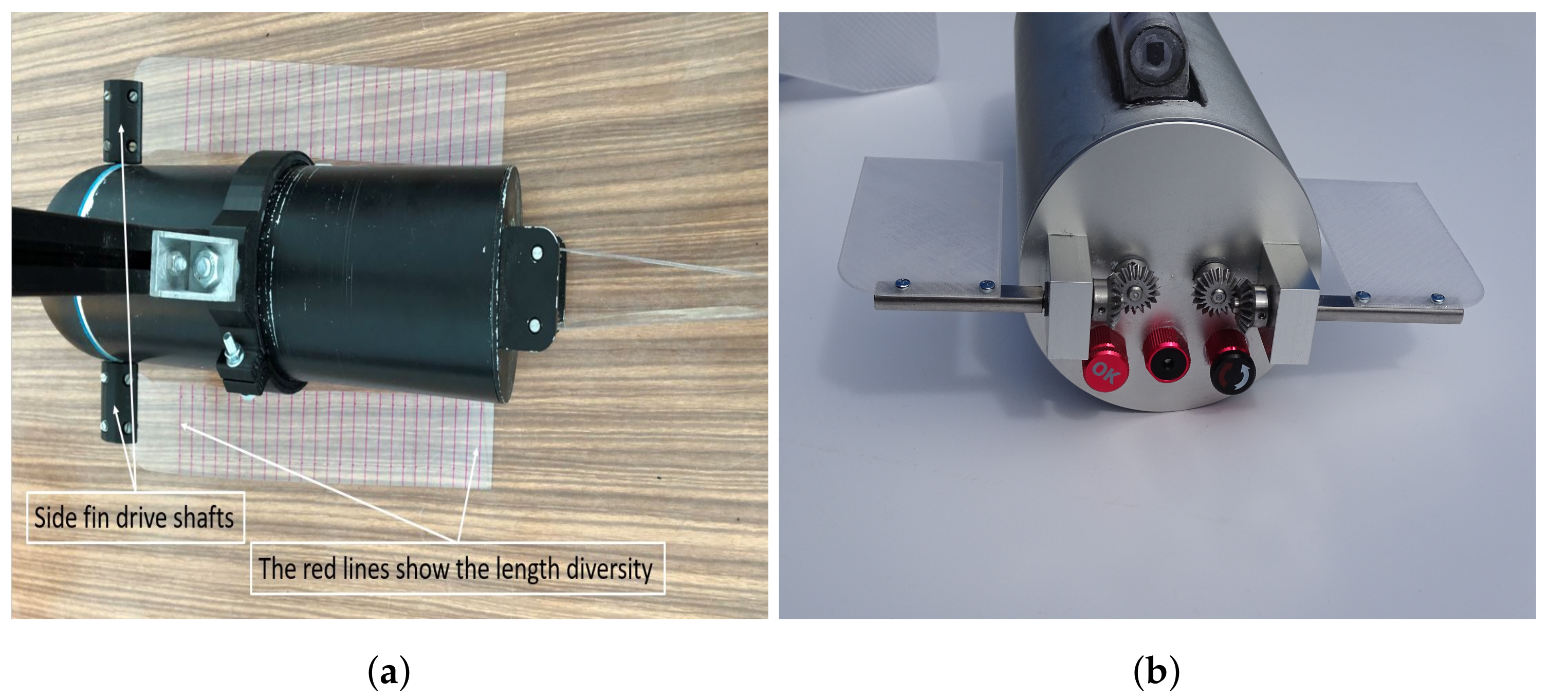
3.1. The Side Fins Construction and Control Algorithm

The test were provided for three values of the fin thickness: 1 mm, 0.75 mm, 0.5 mm; and three values of the fin width: 55 mm, 45 mm, 35 mm. The thickness above 1 mm was too stiff for that type of servo while the thickness below 0.5 mm and the width: 45 mm and 35 mm give low values of fin flexibility. That is why, for fin thickness equal to 0.5 mm, only the results for the widest fin (55 mm) are presented. All the fin’s length was changed from 330 mm to 80 mm with step 10 mm, as depicted in Figure 3, where the red lines show the length diversity. The maximal length of the tested side fins was limited by the length of the hull of the BUUV. Longer side fins than the BUUV hull dimensions caused an interaction with the tail fins. The tested fins were made from the same material (polymethyl methacrylate) due to easy design process of many various side area and shape. The parameters: density: 1.18 (g/cm 3 ); tensile strength: 70 (MPa); flexural modulus (GPa): 2.9; help to estimate Young’s modulus for calculating the stiffness coefficient [35]. Thanks to the shatter resistance, it can be used for many cycles of fin oscillations. It also provides outstanding stability against environmental conditions. Further, their transparency is convenient for the particle image velocimetry (PIV) technique. The laser can highlight both sides of the fin no matter how it is deflected (see Figure 2b).
The BUUV’s side fins are powered by a dynamixel AX-12A (http://www.dynamixel.com/, accessed on 15 July 2022) servomechanism installed inside the hull. The torque from the servomechanisms to the fins is transmitted through the bevel gear, as shown in Figure 3b. The Dynamixel AX-12+ has a stall torque (M) of 1.5 Nm (at 12 V, 1.5 A) and a top no load speed of 59 revolutions per minute (rpm). After preliminary tests, the maximal amplitude of the fin movement was established to 40 at the leading edge. The amplitude of the trailing edge, on the other hand, is proportional to the size and, hence, to the flexibility of the fin, so it was quantified using a non-invasive image processing method. The frequency of fin oscillation is determined by the servo’s rotating velocity, as well as the fin angle of attack. Fin frequency oscillation may be achieved at up to 4.5 Hz at unloaded speed and leading edge angle of 40 .

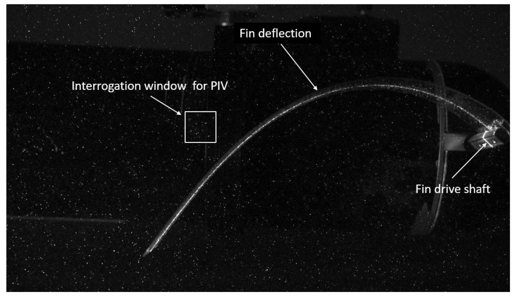
3.2. Image Processing Method
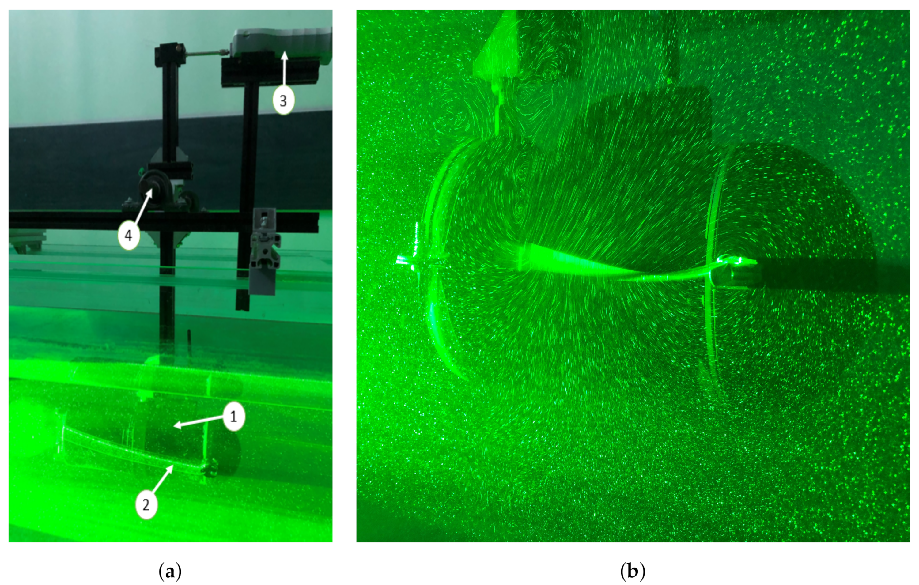
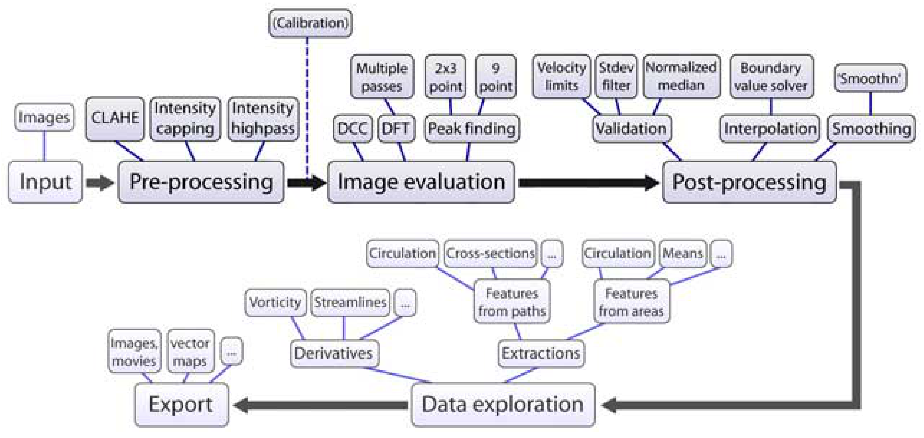
To determine fin displacement and deflection, a non-invasive image processing method was applied. An industrial high speed camera was employed to record particle movement as well as fin displacement while lit by a linear laser (see Figure 4). For the PIV approach, the camera records the motion of the fin, as well as the displacement of the particle. The fin motion is utilised to analyse kinematics, particularly the amplitude of the trailing edge, as presented in the author’s publications [32,43], whereas the PIV approach is employed for a more in-depth investigation of the fluid–fin interaction.

3.3. PIV Method

PIV is a non-invasive visual approach for determining fluid velocity in a specified area. The PIVLab programme was utilised for the analysis [44]. To compute the template displacement in each frame from the vision system, the normalised cross-correlation function based on grey-scale images is used. The size of an interrogation window (see Figure 4) is determined by the fluid velocity, the region of research, and the camera performance. Calibration is also supplied depending on frames per second and a reference distance. Because of their neutral buoyancy and small size (diameter 10 μ m), the test markers had no effect on the nature of the fluid movement. The markers are made from transparent glass balls that are encircled by silver. This, in conjunction with a 1 W green linear laser, ensures a high enough refraction to record particle velocity by a camera with a resolution of 2048 × 1952 at 1000 frames per second. The seed density (the number of markers in the area unit) has been set to guarantee that about 10 markers are within the interrogation window. The image shown in Figure 4 was acquired for an illuminated plane perpendicular to the side fin and used as input data for PIV analysis. To compute the velocity field, two successive pictures are analysed.
The PIV analysis typically consists of three main steps (image pre-processing, image evaluation, and post-processing). The workflow adopted from paper the [44] is presented in Figure 5, starting with image input and pre-processing options, and then continuing to the image evaluation, post-processing, and data exploration [45]. It allows calculating the velocity distribution within particle image pairs as well as to derive, display, and export multiple parameters of the flow pattern. In the situation of interrogation window size limitations in the cross correlation function, the PIV approach based on Artificial Intelligence [46] can be utilised for boundary layer analysis.
After achieving the state-of-the-art requirements [45], the PIV approach was employed to calculate water velocity in a fin–fluid interaction area. Furthermore, fluid turbulence analysis was provided to observe the characteristics of the flow, particularly at the trailing edge of the fin.

4. Results and Discussion

The next sub-paragraphs present all of the results obtained via image processing, the PIV method, and direct measurement of thrust.

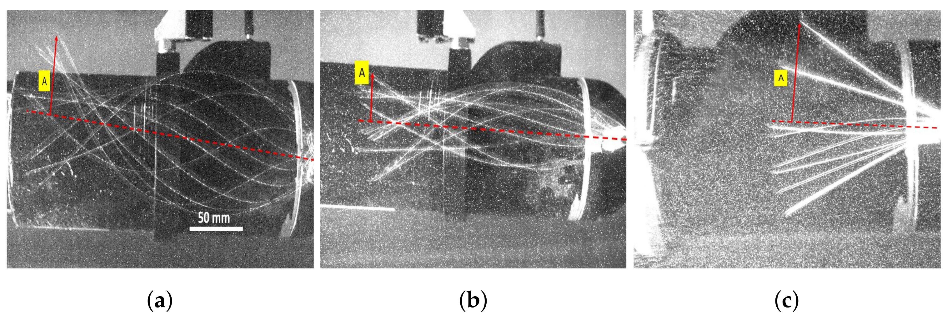
4.1. Kinematic Parameters Based on Image Processing
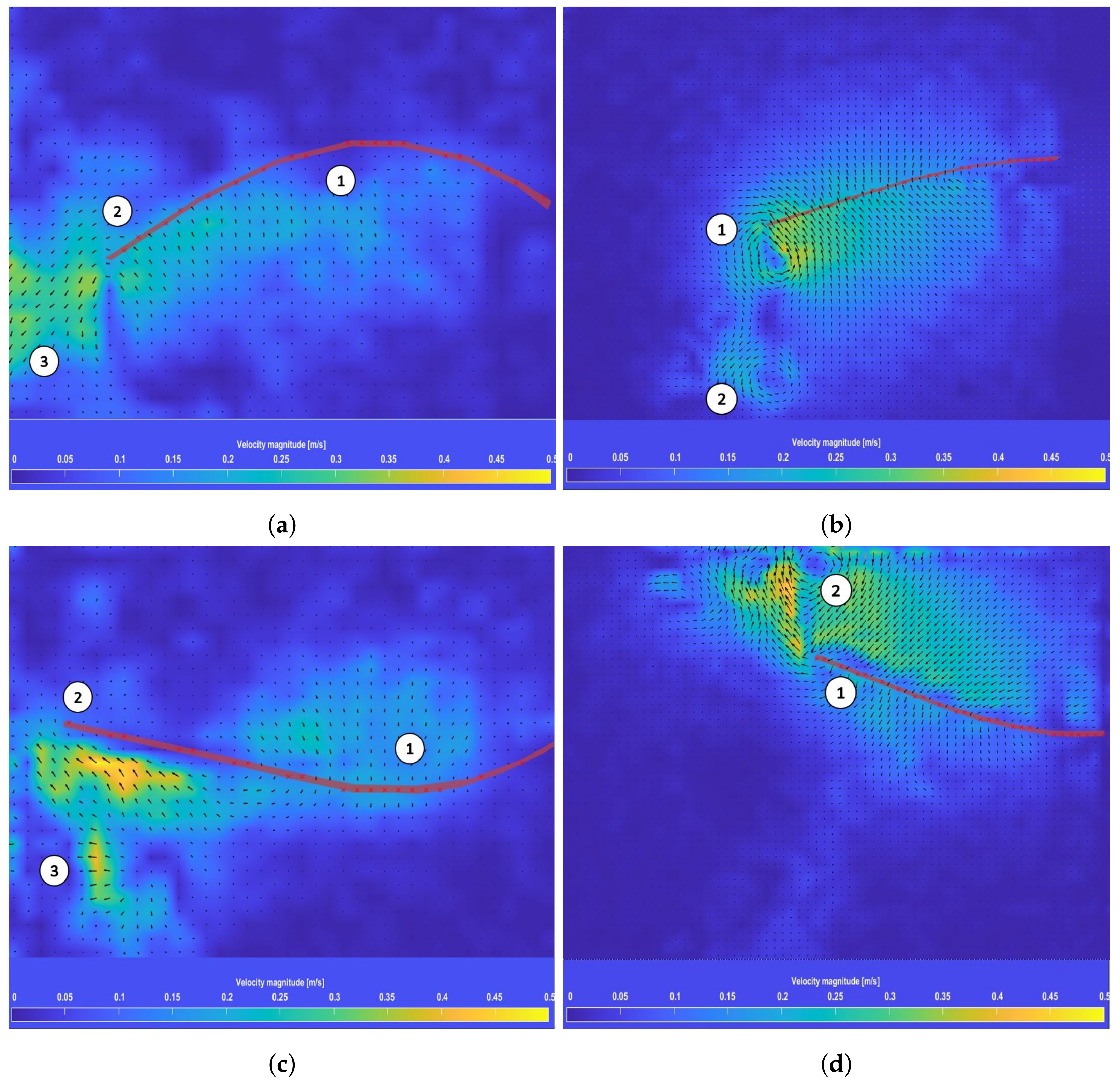
In Figure 6, an example of fins deflection is presented for the fin length equal to: 300 mm (see Figure 6a), 250 mm (see Figure 6b), and 150 mm (see Figure 6c). The photos were created by combining a series of images saved in a 2048 × 1952 matrix, with each pixel saved in u i n t 8 data format. As a result, when a u i n t 8 matrix sequence is added to one matrix, the brightness of the final result exhibited as an image varies depending on the magnification and number of recorded markers. The sequence of fin deflection allows the amplitude of a fin trailing edge, denoted by the capital letter A in Figure 6 on the yellow background, to be measured. The amplitude of the trailing edge of the fin is greatest (equivalent to 63 mm) for the fin length of 150 mm as shown in Figure 6c. The smallest amplitude of the fin trailing edge (42 mm) was measured for fin lengths of 250 mm (Figure 6b). The kinematic analysis shown in (Figure 6a) demonstrates that the amplitude of the trailing edge is 60 mm.
The amplitude of the fin trailing edge combined with the known frequency of fin oscillation can be used to calculate the Strouhal number (see Equation (4)). A fluid velocity is the most perplexing variable, especially for unmoving (fixed) BUUV. This can be measured using the PIV method in the area of interaction between fins and fluid, as shown in the next paragraph.

4.2. PIV Results

The result from the PIV analysis presented in Figure 7 was provided for fin dimensions: 55 mm width, 0.75 mm thickness, and two lengths 250 mm (Figure 7a,c) and 150 mm (Figure 7b,d) when moving the fin up (Figure 7a,b) and down (Figure 7c,d). The fluid velocity was calculated based on PIV method as an average value of velocity vectors in the area of the interaction between fins and fluid. All velocity vectors depicted in Figure 7 as arrows can be calculated in a selected area. Still, again the difficulties are connected with the size and shape of the area. For example, the shorter fins (e.g., 150 mm length) moved the fluid in a larger vertical area, but as presented in Figure 7b,d also generate turbulence. The swirls are especially noticeable at the fin tips (numbered 1 in Figure 7b), while for the longer fins, due to their flexibility, the flow at the fin tips is more laminar (see region numbered 2 in Figure 7a,c).
The regions marked by number 3 in Figure 7a,c show the velocity vectors for fin length 250 mm. There are no swirls in comparison to PIV results as presented in Figure 7b,d. The velocity vectors for longer fins are created into two steps (regions marked by numbers 1 and 3 in Figure 7a,c). During the first phase, the middle part of the fin attracts the water giving preliminary velocity value and direction (see region number 1 in Figure 7a,c), while in the second phase the velocity is added to the fin trailing edge velocity. As a result, the velocity vectors are formed with reverse direction than BUUV movement. It is worth mentioning that in each swirl, the energy is dissipated, so it is not desired from an energy efficiency point of view. This is useful for analysing if the flow is laminar or turbulent, and if it is turbulent, where is the energy dissipated most? Taking into account the results presented for the length of the fins 150 mm (Figure 7b,d), it can be seen that the turbulence occurs not only at the trailing edge of the fin, but also additional turbulence is generated as indicated in these graphs with the number 2.
Every test result can be analysed as an average value of fluid velocity but also the velocity component can be calculated. It is desirable to reduce the perpendicular component of the velocity vectors with respect to the direction of movement while maximising the longitudinal component.
The calculation of the fluid mean velocity for the desired area gives the fluid velocity value for two pairs of images from 0.06 m/s to 0.1 m/s, which gives the Strouhal number range from 0.31 up to 1.89 for the fin length 250 mm. The same calculation (based on Equation (4)) provides the Strouhal number with range from 0.27 up to 1.36 for fin length 150 mm. Because the measurements were performed for fixed BUUV it is expected that the velocity in an area of analysis will change proportionally to the BUUV hull velocity, giving the lower value of the Strouhal number. Although the measured fins have the same length diverse with 10 mm step it has an impact on: the non-dimensional parameter (K) defining the shape of the fin; the stiffness coefficient (see Equation (2)); the Reynolds number (see Equation (3)); and, as a consequence, has an impact on the Strouhal number (see Equation (4)). Although the Strouhal Number can be used to compare the energy efficiency of a propulsion system with a marine animal, the next paragraph presents direct thrust measurements.

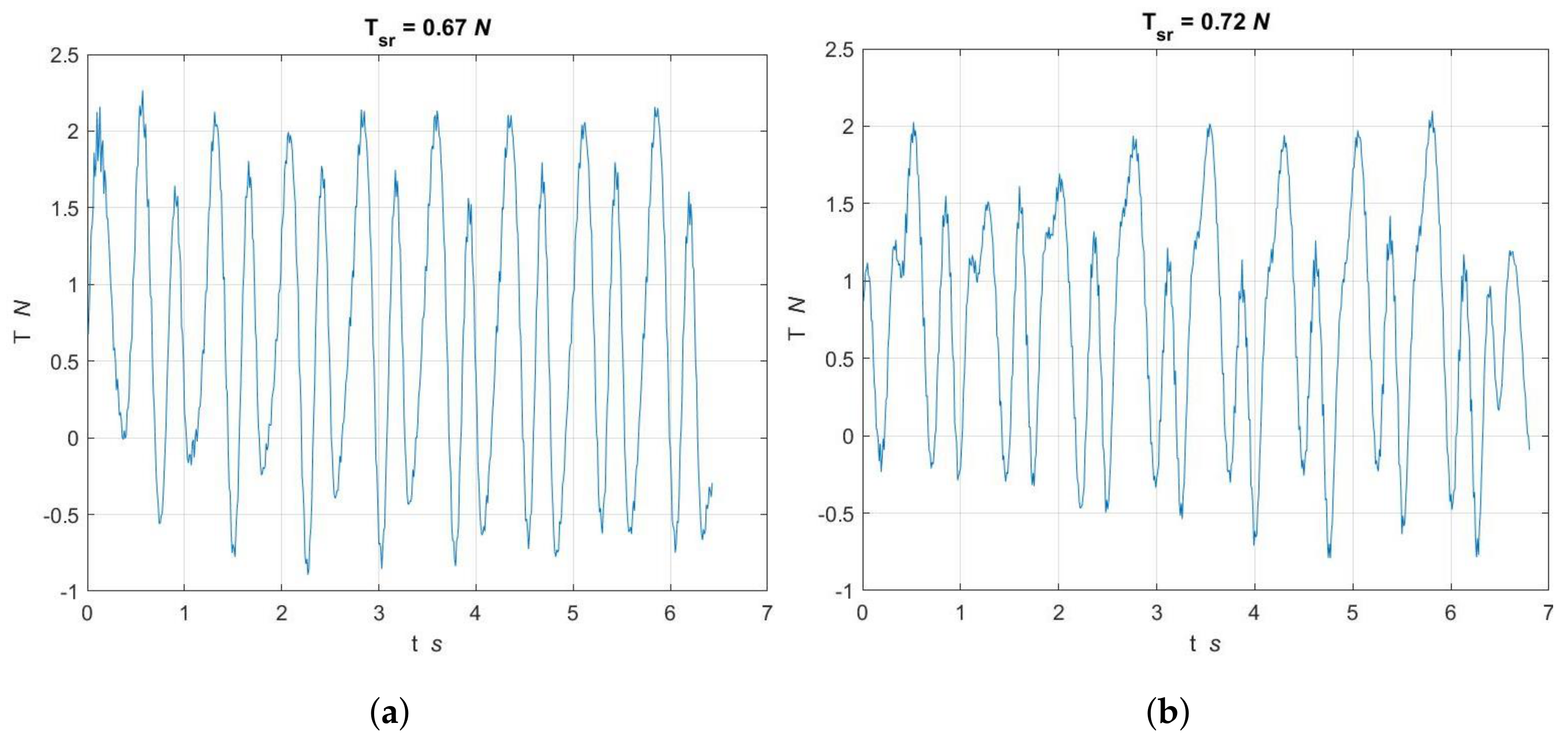
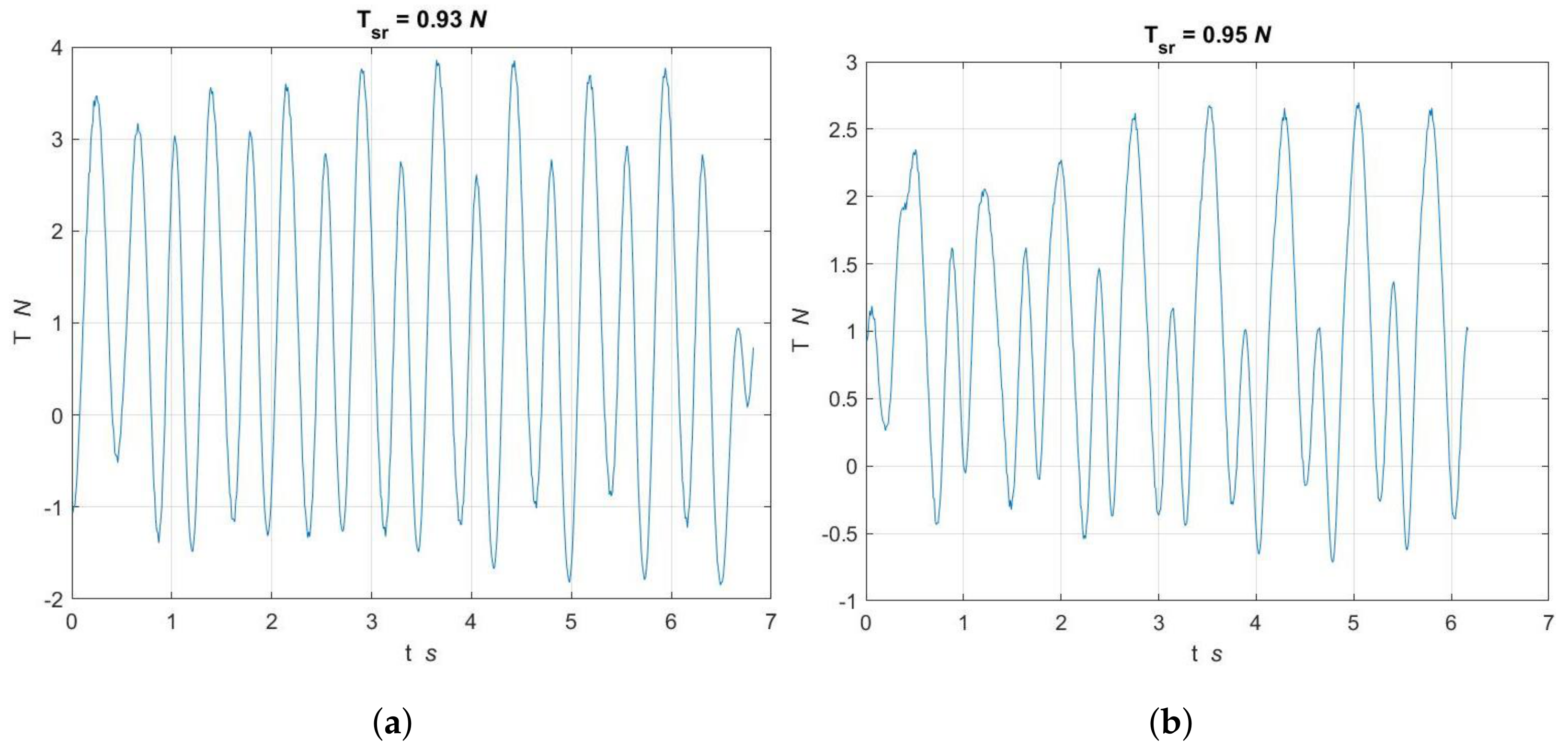
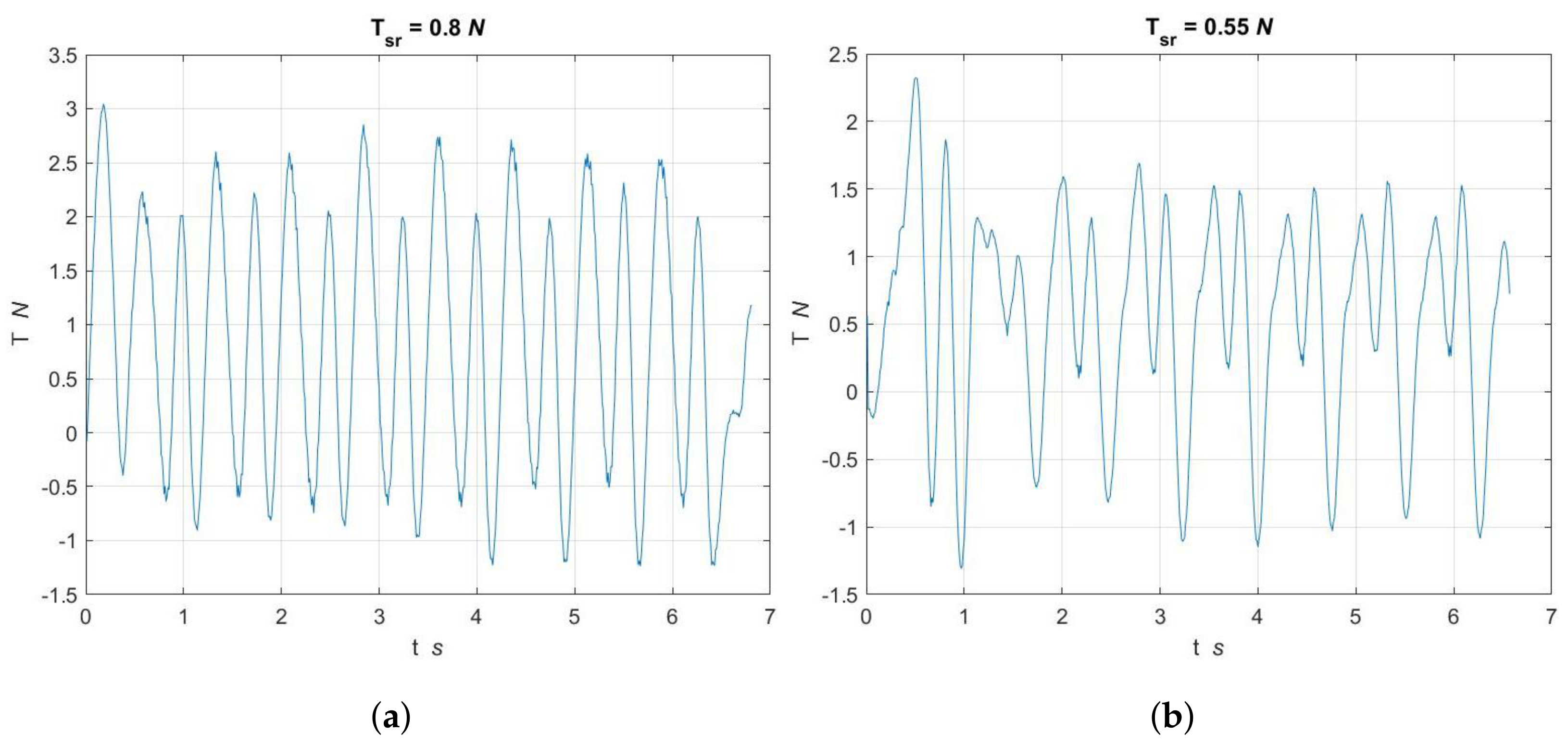
4.3. Direct Thrust Measurements

During the tests, it was observed (as presented in Table 1 and Figure 8 and Figure 9) a high sensitivity to changing the fins length. In Figure 8, the mean thrust is presented as a function of the fins length for different width (55 mm, 45 mm, and 35 mm) and thickness equal to 1 mm (left graph) and and thickness equal to 0.75 mm (right graph). The highest value of mean thrust is observed for the fins width of 55 mm, which can be explained by the greater side area of the fins. As the measurements revealed, to ensure the maximum value of mean thrust for a longer fin, the width should be changed. Further, the same relation can be observed for fin dimensions: 0.5 mm thickness, and 55 mm width, where three maximal values for fin length are equal to 100 mm, 220 mm, and 330 mm (see last column in Table 1). However, the most interesting relationships cab be seen in Figure 9 where results for fins with the same width but three different thickness (1.00 mm, 0.75 mm, and 0.50 mm) are presented. The stiffest fin (indicated as F i n 1.00 × 55 ) has one maximal value for the fin length equal to 150 mm and the second, almost the same maximal value for the fin length equal to 330 mm (longer fins were not analysed due to the BUUV hull length). For the fin thickness equal to 0.75 mm for every width of tested fins, two maximum mean thrust values are indicated as a function of the fin length. It can be seen that the second local maximal value ( T s r = 0.72 N for c = 290 mm) is higher than the first local maximal value ( T s r = 0.67 N for c = 140 mm). For the thinnest fin (indicated as F i n 0.50 × 55 ) three local maxima of the mean thrust in relation to fins’ length ( T s r = 0.43 N for c = 100 mm, T s r = 0.51 N for c = 220 mm, T s r = 0.43 N for c = 330 mm) are observed.
Based on the tests provided, it can be seen that the maximum mean value can be achieved for different fin lengths of the same with and thickness, as well as the same control algorithm. As distinguished in Table 1 and Figure 8 and Figure 9), the maximal value of mean thrust is correlated with the fin dimensions. The differences between the maximal value of mean thrust can be explained based on an analysis of the graph presenting the thrust as a function of time (see Figure 10b, Figure 11b and Figure 12b), where the nature of the thrust changes are presented. In Figure 10a, Figure 11 and Figure 12b, the chosen characteristics are presented among 625 measurements depicted in Table 1, just to highlight the nature of changes. The chosen relations indicate the mean value depicted above each graph.
Taking into consideration the thrust characteristics presented in Figure 10a,b it can be seen that both have almost the same mean thrust (0.93 N and 0.95 N), but the range of maximal and minimal thrust varies. For the fin length 150 mm (Figure 10a), the thrust range is from +3.7 N to −1.8 N, while for the fin length 330 mm the thrust range is from +2.6 N to −0.8 N. This indicates that the same thrust can be achieved with different energy consumption, while the difference is dissipated in the swirls. The next example presents the comparable minimum value of the thrust range with the mean value proportional to the differences in maximal values of the thrust (Figure 11a,b). It can also be observed that comparable minimum value of the thrust range (−0.5 N) with comparison to the high range (2.25 N) as depicted in Figure 12a and (2.0 N) as depicted in Figure 12b gives mean thrust equal to T = 0.67 N and 0.72 N, respectively. This is caused by the characteristic shape and this factor will be tested in the next step of research.
The fin movement can be divided into two parts: the working and the return movement. As it can be seen in Figure 10a, Figure 11 and Figure 12b there are significant differences between the thrust amplitude, even if the average one value is comparable. There are two methods for increasing the mean thrust force: the first is to increase the maximal thrust value throughout the movement in both cycles, and the second is to transfer all the characteristics to one region of the graph. In that case (more desirable due to better energy efficiency), the propulsion system generates only thrust in one direction during the working and return movements.

5. Conclusions and Future Work

To summarise, a wide range of fin shapes were examined, and a thorough analysis was presented using direct trust measurements, image processing, and the PIV approach. The number of design and control variables was reduced to highlight the impact of fin dimensions on side propulsion system performance. The reported findings were picked from thousands of observations to demonstrate the dependence of thrust created by a single flexible fins as a function of fin dimensions in time domain. Because of the non-linear relationships of many factors, the dependencies between fin dimensions demonstrate that maintaining high efficiency propulsion system settings is a difficult undertaking. As a result, nowadays stiff fins are frequently used in BUUV constructions. The stiffness fin is less efficient than the flexible fin, but the parameters are less dependent on the construction data, therefore the thrust may be modified for underwater vehicle velocity control by simply adjusting the control data.
Only one dimension of the side fin will be examined for different control algorithms in the following step of the project. The angle of attack and frequency of fin movement will then be modified to maintain the high energy-efficient propulsion system characteristics. As a final result, the propulsion system will be low noise (due to the one flexible side fin) and high energy efficient.

Funding

The BUUV was designed during the Polish Ministry of Defense competition. The laboratory tunnel was funded by the Polish Ministry of Defence Grand entitled “Model studies of the characteristics of an undulating propulsion system” provided in 2018–2021.

Acknowledgments

The BUUV swarm was designed by the team from Polish Naval Academy during the Minister of Defence competition in 2021.

Conflicts of Interest

The authors declare no conflict of interest.

Abbreviations

The following abbreviations are used in this manuscript:
BUUVBiomimetic Unmanned Underwater Vehicle
PIVParticle Image Velocimetry
RPMRevolutions Per Minute
FSIFluid–Structure Interaction.

References

  1. Mannam, N.P.B.; Krishnankutty, P. Biological Propulsion Systems for Ships and Underwater Vehicles. In Propulsion Systems; IntechOpen: London, UK, 2019; p. 113. [Google Scholar] [CrossRef] [Green Version]
  2. He, J.; Cao, Y.; Huang, Q.; Pan, G.; Dong, X.; Cao, Y. Effects of Bionic Pectoral Fin Rays’ Spanwise Flexibility on Forwarding Propulsion Performance. J. Mar. Sci. Eng. 2022, 10, 783. [Google Scholar] [CrossRef]
  3. Sitorus, P.E.; Nazaruddin, Y.Y.; Leksono, E.; Budiyono, A. Design and Implementation of Paired Pectoral Fins Locomotion of Labriform Fish Applied to a Fish Robot. J. Bionic Eng. 2009, 6, 37–45. [Google Scholar] [CrossRef]
  4. Shi, L.; Guo, S.; Mao, S.; Yue, C.; Li, M.; Asaka, K. Development of an Amphibious Turtle-Inspired Spherical Mother Robot. J. Bionic Eng. 2013, 10, 446–455. [Google Scholar] [CrossRef]
  5. Szymak, P.; Przybylski, M. Thrust measurement of biomimetic underwater vehicle with undulating propulsion. Sci. J. Pol. Nav. Acad. 2018, 213, 69–82. [Google Scholar] [CrossRef]
  6. Salazar, R.; Quintana, R.; Abdelkefi, A. Role of Electromechanical Coupling, Locomotion Type and Damping on the Effectiveness of Fish-Like Robot Energy Harvesters. Energies 2021, 14, 693. [Google Scholar] [CrossRef]
  7. Morawski, M.; Słota, A.; Zając, J.; Malec, M. Fish-like shaped robot for underwater surveillance and reconnaissance–Hull design and study of drag and noise. Ocean Eng. 2020, 217, 107889. [Google Scholar] [CrossRef]
  8. Liu, G.; Dong, H. Effects of tail geometries on the performance and wake pattern in flapping propulsion. In Proceedings of the ASME 2016 Fluids Engineering Division Summer Meeting collocated with the ASME 2016 Heat Transfer Summer Conference and the ASME 2016 14th International Conference on Nanochannels, Microchannels, and Minichannels, Washington, DC, USA, 10–14 July 2016; Volume 50299, p. V01BT30A002. [Google Scholar] [CrossRef] [Green Version]
  9. Malec, M.; Morawski, M.; Zając, J. Fish-like swimming prototype of mobile underwater robot. J. Autom. Mob. Robot. Intell. Syst. 2010, 4, 25–30. [Google Scholar]
  10. Morawski, M.; Malec, M.; Szymak, P.; Trzmiel, A. Analysis of Parameters of Traveling Wave Impact on the Speed of Biomimetic Underwater Vehicle. In Solid State Phenomena; Trans Tech Publications: Freienbach, Switzerland, 2014; Volume 210, pp. 273–279. [Google Scholar]
  11. Szymak, P.; Malec, M.; Morawski, M. Directions of development of underwater vehicle with undulating propulsion. Pol. J. Environ. Stud. 2010, 19, 107–110. [Google Scholar]
  12. Przybylski, M.; Szymak, P.; Kitowski, Z.; Piskur, P. Comparison of Different Course Controllers of Biomimetic Underwater Vehicle with Two Tail Fins. In Advanced, Contemporary Control; Springer: Berlin/Heidelberg, Germany, 2020; pp. 1507–1518. [Google Scholar]
  13. Hożyń, S.; Zalewski, J. Shoreline Detection and Land Segmentation for Autonomous Surface Vehicle Navigation with the Use of an Optical System. Sensors 2020, 20, 2799. [Google Scholar] [CrossRef]
  14. Hożyń, S. A Review of Underwater Mine Detection and Classification in Sonar Imagery. Electronics 2021, 10, 2943. [Google Scholar] [CrossRef]
  15. Jaskolski, K. Methodology for Verifying the Indication Correctness of a Vessel Compass Based on the Spectral Analysis of Heading Errors and Reliability Theory. Sensors 2022, 22, 2530. [Google Scholar] [CrossRef] [PubMed]
  16. Szymak, P.; Praczyk, T.; Pietrukaniec, L.; Hożyń, S. Laboratory stand for research on mini CyberSeal. Meas. Autom. Monit. 2017, 63, 228–233. [Google Scholar]
  17. Tytell, E.D.; Hsu, C.Y.; Williams, T.L.; Cohen, A.H.; Fauci, L.J. Interactions between internal forces, body stiffness, and fluid environment in a neuromechanical model of lamprey swimming. Proc. Natl. Acad. Sci. USA 2010, 107, 19832–19837. [Google Scholar] [CrossRef] [PubMed] [Green Version]
  18. Hozyn, S. An Automated System for Analysing Swim-Fins Efficiency. Nase More 2020, 67, 10–17. [Google Scholar] [CrossRef]
  19. Grzadziela, A.; Szymak, P.; Piskur, P. Method for assessing the dynamics and efficiency of diving fins. Acta Bioeng. Biomech. 2020, 22, 139–150. [Google Scholar] [CrossRef] [PubMed]
  20. Grządziela, A.; Kluczyk, M.; Batur, T. The Stand for Fin Drives Energy Testing. Pedagogica 2021, 93, 250–262. [Google Scholar] [CrossRef]
  21. Blondeaux, P.; Fornarelli, F.; Guglielmini, L.; Triantafyllou, M.; Verzicco, R. Vortex structures generated by a finite-span oscillating foil. In Proceedings of the 43rd AIAA Aerospace Sciences Meeting and Exhibit, Reno, NV, USA, 10–13 January 2005; p. 84. [Google Scholar] [CrossRef]
  22. Piskur, P.; Szymak, P.; Kitowski, Z.; Flis, L. Influence of fin’s material capabilities on the propulsion system of biomimetic underwater vehicle. Pol. Marit. Res. 2020, 179–185. [Google Scholar] [CrossRef]
  23. Matta, A.; Pendar, H.; Battaglia, F.; Bayandor, J. Impact of caudal fin shape on thrust production of a Thunniform swimmer. J. Bionic Eng. 2020, 17, 254–269. [Google Scholar] [CrossRef]
  24. Piskur, P.; Szymak, P.; Przybylski, M.; Naus, K.; Jaskólski, K.; Żokowski, M. Innovative energy-saving propulsion system for low-speed biomimetic underwater vehicles. Energies 2021, 14, 8418. [Google Scholar] [CrossRef]
  25. Thekkethil, N.; Sharma, A.; Agrawal, A. Self-propulsion of fishes-like undulating hydrofoil: A unified kinematics based unsteady hydrodynamics study. J. Fluids Struct. 2020, 93, 102875. [Google Scholar] [CrossRef]
  26. Gater, B.; Bayandor, J. Amplitude Effects on Thrust Production for Undulatory Swimmers. In Proceedings of the APS Division of Fluid Dynamics Meeting Abstracts, Denver, CO, USA, 19–21 November 2017; p. L9.007. [Google Scholar]
  27. Piskur, P.; Szymak, P.; Flis, L.; Sznajder, J. Analysis of a Fin Drag Force in a Biomimetic Underwater Vehicle. Nase More 2020, 67, 192–198. [Google Scholar] [CrossRef]
  28. Bergmann, M.; Iollo, A. Modeling and simulation of fish-like swimming. J. Comput. Phys. 2011, 230, 329–348. [Google Scholar] [CrossRef]
  29. Kubit, A.; Trzepieciński, T.; Kiciński, R.; Jurczak, K. Three-Dimensional Smooth Particle Hydrodynamics Modeling and Experimental Analysis of the Ballistic Performance of Steel-Based FML Targets. Materials 2022, 15, 3711. [Google Scholar] [CrossRef] [PubMed]
  30. Behbahani, S.B.; Tan, X. Design and dynamic modeling of electrorheological fluid-based variable-stiffness fin for robotic fish. Smart Mater. Struct. 2017, 26, 085014. [Google Scholar] [CrossRef]
  31. Engels, T.; Kolomenskiy, D.; Schneider, K.; Sesterhenn, J. Numerical simulation of vortex-induced drag of elastic swimmer models. Theor. Appl. Mech. Lett. 2017, 7, 280–285. [Google Scholar] [CrossRef]
  32. Jurczyk, K.; Piskur, P.; Szymak, P. Parameters identification of the flexible fin kinematics model using vision and Genetic Algorithms. Pol. Marit. Res. 2020, 39–47. [Google Scholar] [CrossRef]
  33. Eloy, C. Optimal Strouhal number for swimming animals. J. Fluids Struct. 2012, 30, 205–218. [Google Scholar] [CrossRef] [Green Version]
  34. Buckingham, E. The principle of similitude. Nature 1915, 96, 396–397. [Google Scholar] [CrossRef] [Green Version]
  35. Kiciński, R.; Kruszkowska, E.O.; Szturomski, B.; Jurczak, W. Stand for Biomimetic Swimming Fins Fatigue Testing. Preprints 2022. [Google Scholar] [CrossRef]
  36. Szturomski, B. Dynamic characteristics of high quality steel in Johnson-Cook’s model for fast processes simulation in CAE programs. In Solid State Phenomena; Trans Tech Publications: Freienbach, Switzerland, 2015; Volume 236, pp. 31–38. [Google Scholar]
  37. Reynolds, O. XXIX. An experimental investigation of the circumstances which determine whether the motion of water shall be direct or sinuous, and of the law of resistance in parallel channels. Philos. Trans. R. Soc. Lond. 1883, 174, 935–982. [Google Scholar]
  38. Baik, Y.S.; Bernal, L.P. Experimental study of pitching and plunging airfoils at low Reynolds numbers. Exp. Fluids 2012, 53, 1979–1992. [Google Scholar] [CrossRef]
  39. Triantafyllou, G.S.; Triantafyllou, M.S.; Grosenbaugh, M.A. Optimal thrust development in oscillating foils with application to fish propulsion. J. Fluids Struct. 1993, 7, 205–224. [Google Scholar] [CrossRef]
  40. Maertens, A.P.; Triantafyllou, M.S.; Yue, D.K.P. Efficiency of fish propulsion. Bioinspir. Biomimetics 2015, 10, 046013. [Google Scholar] [CrossRef] [PubMed] [Green Version]
  41. Bevilaqua, P.; Yam, C. Propulsive Efficiency of Wake Ingestion. J. Propuls. Power 2020, 36, 517–526. [Google Scholar] [CrossRef]
  42. Piskur, P.; Szymak, P.; Sznajder, J. Identification in a laboratory tunnel to control fluid velocity. In Advanced, Contemporary Control; Springer: Berlin/Heidelberg, Germany, 2020; pp. 1543–1552. [Google Scholar]
  43. Piskur, P. Strouhal Number Measurement for Novel Biomimetic Folding Fins Using an Image Processing Method. J. Mar. Sci. Eng. 2022, 10, 484. [Google Scholar] [CrossRef]
  44. Thielicke, W.; Stamhuis, E. PIVlab–towards user-friendly, affordable and accurate digital particle image velocimetry in MATLAB. J. Open Res. Softw. 2014, 2, 1. [Google Scholar] [CrossRef] [Green Version]
  45. Thielicke, W.; Sonntag, R. Particle Image Velocimetry for MATLAB: Accuracy and enhanced algorithms in PIVlab. J. Open Res. Softw. 2021, 9, 1. [Google Scholar] [CrossRef]
  46. Majewski, W.; Wei, R.; Kumar, V. Developing particle image velocimetry software based on a deep neural network. J. Flow Vis. Image Process. 2020, 27, 4. [Google Scholar] [CrossRef]
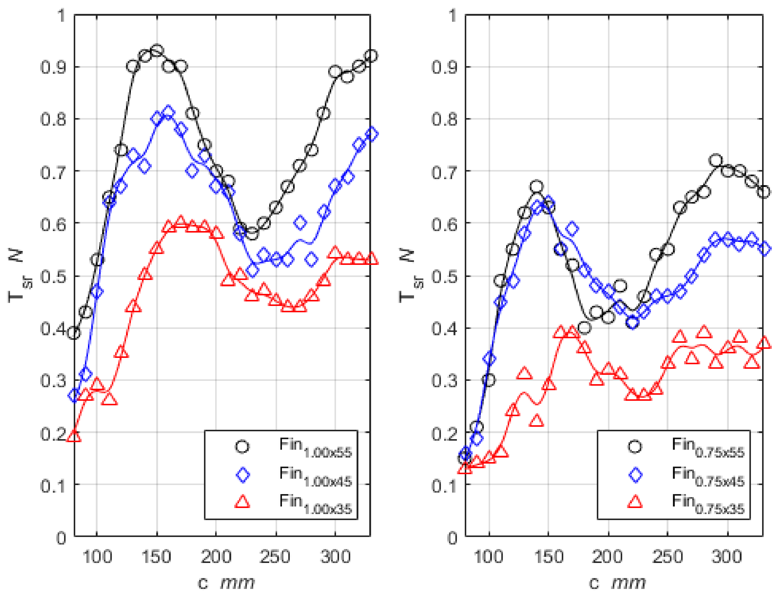
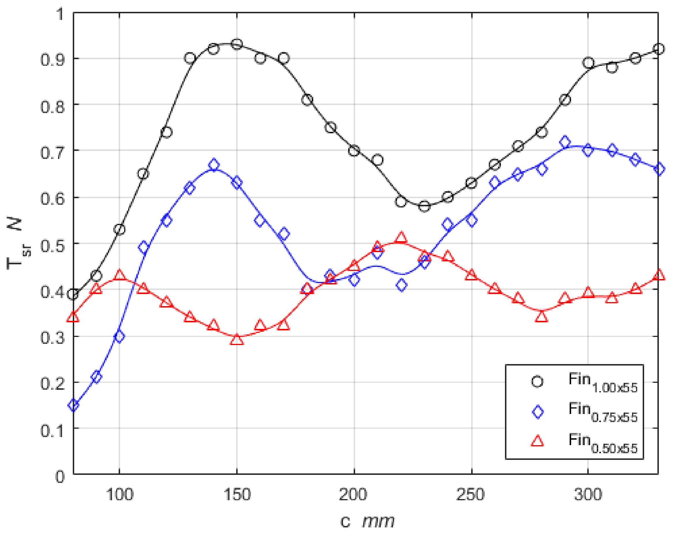
Figure 1. BUUV with propulsion system made of two flexible tail and side fins (a) top back view; (b) front view; and (c) small version.
Energies 15 05783 g001
Figure 2. The laboratory water tunnel and green linear laser highlighting one of the side fin (a): 1—BUUV, 2—the side fin, 3—the force sensor, and 4—a ball bearing; (b) particles illuminated by linear green laser.
Energies 15 05783 g002
Figure 3. Top view of the BUUV with side fins (a) and front view of (without bow dome) the propeller shaft with bevel gear (b).
Energies 15 05783 g003
Figure 4. The example of input data for analysis with highlight markers and illuminated the fin deflection.
Energies 15 05783 g004
Figure 5. Overview of the workflow in PIVlab and the implemented features [44].
Energies 15 05783 g005
Figure 6. Fins deflections for different length: (a) 300 mm, (b) 250 mm, and (c) 150 mm.
Energies 15 05783 g006
Figure 7. PIV analysis for fin length: 250 mm when moving the fin up (a) and down (c), 150 mm when moving the fin up (b) and down (d).
Energies 15 05783 g007
Figure 8. Thrust mean ( T s r ) as a function of the fins length for different fin widths and thicknesses.
Energies 15 05783 g008
Figure 9. Thrust mean ( T s r ) as a function of the fins length for fin widths equal to 55 mm, and different fin thicknesses.
Energies 15 05783 g009
Figure 10. The thrust value as a function of time for fins dimensions: width 55 mm, thickness 1 mm and length: (a) 150 mm; (b) 330 mm.
Energies 15 05783 g010
Figure 11. The thrust value as a function of time for fins dimensions: width 45 mm, thickness 1 mm and length: (a) 160 mm; (b) length 230 mm.
Energies 15 05783 g011
Figure 12. The thrust value as a function of time for fins dimensions: width 55 mm, thickness 0.75 mm and length: (a) 140 mm; (b) 290 mm.
Energies 15 05783 g012
Table 1. Thrust mean results ( T s r ) measured for different fin dimensions.
Mean Thrust T sr N
Fin DimensionsThickness mm × Width mm
Length mm1.0 × 551.0 × 451.0 × 350.75 × 550.75 × 450.75 × 350.5 × 55
3300.930.770.530.660.550.370.43
3200.900.700.530.680.570.330.40
3100.880.690.530.700.560.380.38
3000.890.670.540.700.570.360.39
2900.810.620.490.720.570.330.38
2800.740.530.460.660.540.390.34
2700.710.600.440.650.500.340.38
2600.670.530.440.630.470.380.40
2500.630.530.450.550.460.330.43
2400.600.540.470.540.460.280.47
2300.580.510.460.460.430.270.47
2200.590.580.500.410.410.270.51
2100.680.660.490.480.440.310.49
2000.700.670.580.420.470.320.45
1900.750.730.590.430.480.300.42
1800.810.700.590.400.510.360.40
1700.900.780.600.520.590.390.32
1600.900.810.590.550.550.390.32
1500.930.800.550.630.640.290.29
1400.920.710.500.670.630.220.32
1300.900.730.440.620.580.310.34
1200.740.670.350.550.490.240.37
1100.650.640.260.490.450.160.40
1000.530.470.290.300.340.150.43
900.430.310.270.210.190.140.40
800.390.270.190.150.160.130.34
Publisher’s Note: MDPI stays neutral with regard to jurisdictional claims in published maps and institutional affiliations.

