Thermodynamic, Exergetic and Thermoeconomic Analyses of Double-Effect LiBr–Water Absorption Refrigeration Systems with a 5 kW High Temperature PEMFC as Heat Source for Data Center Applications

Abstract

Thermodynamic, exergetic and thermoeconomic analyses were performed on two types of double-effect LiBr–water absorption refrigeration systems (ARS) for use with a 5-kW high-temperature proton exchange membrane fuel cell (HT-PEMFC) as a heat source. Proper temperatures of the high-pressure generator, combined generator and condenser, condenser, absorber and evaporator were determined to meet the requirements of constant cooling demands for data center operations. The heat balance of the combined unit of generator and condenser in the industrial double-effect LiBr-water ARS is important for determining the flow rate of the primary vapor refrigerant from the high-pressure generator. The industrial double-effect ARS system, whose analysis has not been studied analytically, outperformed the series double-effect system and provided 6.5 kW of cooling capacity with a coefficient of performance of 0.99. The unit cost of chilled water estimated by the modified productive structure analysis (MOPSA) method is approximately 7.18 USD/GJ (=0.026 US$/kWh). Effective exergetic efficiency of HT-PEMFC with the industrial ARS increases to 57.6% from 47.0%.

1. Introduction

Studies on combined cooling, heating and power (CCHP) systems that integrate single-effect absorption cooling systems (ARS) and low-temperature proton exchange membrane fuel cells (LT-PEMFC) have been conducted by various researchers. For example, a performance analysis of a CCHP system incorporating a 5-kW LT-PEMFC with a single effect ARS was performed by Chen et al. [1]. With a cold water input temperature of 15 °C and an output temperature of 10 °C in the evaporator, a cooling water input temperature of 32 °C in the absorber, a cooling water output temperature of 36 °C in the condenser and a heat source input temperature of 85 °C in the generator as design variables, they have a cooling capacity of 4.6 kW and a coefficient of performance (COP) of 0.67 at the operating temperature of LT-PEMFC, 86 °C. A thermodynamic performance evaluation of the CCHP system based on a 1-kW LT-PEMFC unit and a half-effect LiBr–water ARS was performed by Cozzolino [2]. A COP of 0.425 was obtained at high and low generator temperature of 58.2 °C, high and low absorber temperature of 33 °C, a condenser temperature of 33 °C and an evaporator temperature of 10 °C. On the other hand, a performance analysis of a high-temperature PEMFC (HT-PEMFC) with a single-effect ARS for trigeneration was conducted by Gwak et al. [3]. Their numerical studies showed that the HT-PEMFC system in combination with a single-effect chiller can adequately respond to a variety of power for cooling and heating needs. Recently, a theoretical model was developed to predict the thermal behavior of diffusion-absorption refrigeration system [4].

As can be seen from the analysis results of Chen et al. [1] and Cozzolino [2], the performance and cooling capacity of a LiBr–water ARS that can be used in connection with the PEMFC system depend crucially on the temperature of the heat source; the operating temperature of the absorber, condenser and evaporator; the inlet and outlet temperature of chilled water in the evaporator; and the inlet and outlet of cooling water temperatures. A double- or triple-effect ARS is recommended for a better COP or greater cooling capacity. However, the use of single-, double- or triple-effect ARSs should be chosen based on the temperature of the heat source. Therefore, CCHP systems integrated with LT-PEMFC cannot provide cooling demand with higher COP.

Maryyami and Dehghan [5] studied the performance of half-effect, single-effect, double-effect, and triple-effect LiBr–water ARSs through exergy analysis. They also analyzed how the COP of these refrigeration systems changes with the operating temperature of the generator, condenser or evaporator. At a condenser operating temperature of 33 °C and an evaporator operating temperature of 4 °C, the minimum operating temperature of the generator is about 55 °C for half-effect, 75 °C for single-effect, 140 °C for series and parallel double-effect and 190 °C for triple-effect ARS. Under these conditions, the COP is 0.41 for half-effect, 0.78 for single-effect, 1.15 for series double-effect, 1.22 for parallel double-effect and 1.50 for triple-effect refrigeration systems. Increasing the operating temperature of the condenser to 39 °C at the same evaporator temperature of 4 °C resulted in an increase in the minimum operation temperature of the generator to 65 °C for half effect, 90 °C for single-effect, 165 °C for series double-effect, 155 °C for parallel double-effect and 225 °C for triple-effect ARS. However, detailed heat balance for generators, condensers and evaporators, which is very important to estimate the COP of the ARS, has not been reported.

An exergy analysis of the multi-effect LiBr–water ARS was conducted by Kaynakli et al. [6] and Maryami and Dehghan [5]. Kaynakli et al.′s analysis revealed that exergy destruction in the high-pressure generator increased at higher temperatures of heat sources, and it increases when the condenser and the absorber temperature increased. According to energetic and exergetic analyses of the various multi-effect ARSs [5], they found that the COP and the exergetic efficiency increases from the half effect to the single, double and triple effects. Gebreslassie et al. [7] performed an exergy analysis considering only unavoidable exergy destruction to obtain the maximum achievable performance. They revealed that the largest exergy destruction occurred in the absorbers and generators, especially at higher heat source temperatures. However, exergy analysis alone does not provide sufficient information on ARS operation.

An exergoeconmic analysis of double-effect ARS was performed by Farshi et al. [8]. They found that lower total investment costs are obtained when the high-pressure generator and the evaporator temperature are high and the condenser temperatures as well as the effectiveness of the solution heat exchanger are low. They also found that the product cost flow rate varies compared to those of the total investment cost. Optimization of single-effect LiBr–water ARS using the exergy concept through the annual operating cost was performed by Rubio-Maya et al. [9]. Information on designing the heat exchangers of the LiBr–water ARS was discussed in detail by Florides et al. [10]. However, no researchers have succeeded in obtaining the unit cost of the chilled water obtained from a LiBr–water ARS, and no detailed thermodynamic, exergetic and thermoeconomic analyses of industrial double-effect LiBr–water ARSs have been performed.

Modified production structure analysis (MOPSA) is an exergetic and thermoeconomic analysis method [11]. In MOPSA, the exergy balance equations for thermal system components can be obtained from the first and second laws of thermodynamics. Therefore, if the exergy balance equation including two flows is expressed as the first law of thermodynamics for one flow and the second law of thermodynamics for another flow, the unit cost of “heat” according to the unit cost of supplied electricity can be obtained [12].

In this study, detailed thermodynamic, exergetic and thermoeconomic analyses of a double-effect LiBr–water ARS with a 5-kW HT-PEMFC system were performed under the following requirements of electricity and cooling demands for data center operation. The operating temperature of the HT-PEMFC and the available temperature of the coolant fluid to the generator were 160 °C and 155 °C, respectively. Measured data of thermal properties such as mass flow, temperature and pressure at various state points in the HT-PEMFC system were used in this analysis. The cooling water entering the absorber uses the water cooled in the cooling tower, and the cooling water exiting the condenser enters the cooling tower again. In addition, the temperature of chilled water entering and exiting the evaporator were set to 12 °C and 7 °C, respectively. The industrial double-effect ARS had a high-pressure generator, condenser, combined generator and condenser units, absorber and evaporator and provided 6.5 kW of cooling capacity with a COP of 0.99. The unit cost of chilled water obtained by MOPSA, which depends on the capital cost flow rate of investment and maintenance as well as the unit cost of the supplied electricity to the ARS was 7.18 USD/GJ (=0.026 USD/kWh).

2. Energy, Exergy, Exergy-Balance and Exergy Cost-Balance Equations

2.1. Mass and Energy Conservation

The mass flow into and out of each device must satisfy the following mass and energy conservation equations.

Mass conservation:

$${\displaystyle \sum }_{in}{\dot{m}}_i={\displaystyle \sum }_{out}{\dot{m}}_i$$

(1)

Energy conservation:

$${\dot{Q}}_{cv}+{\displaystyle \sum }_{in}{\dot{H}}_i={\displaystyle \sum }_{out}{\dot{H}}_i+{\dot{W}}_{cv}$$

(2)

In Equation (2), $\dot{H}=\dot{m}h$, and h is enthalpy per unit mass; ${\dot{Q}}_{cv}$ is the heat transfer interaction between a component and the environment; and ${\dot{W}}_{cv}$ is the power.

2.2. Exergy, Exergy-Balance and Cost-Balance Equations

An exergy stream may be decomposed into its thermal and mechanical exergies. These include the exergy losses due to the heat transfer through a non-adiabatic component, and a general exergy-balance equation obtained from the first and second law of thermodynamics may be expressed as [13]:

$$\begin{array}{l}{\dot{E}}_x^{CHE}+({\displaystyle {\displaystyle \sum }_{inlet}}{\dot{E}}_{x,i}^T-{\displaystyle {\displaystyle \sum }_{outlet}}{\dot{E}}_{x,j}^T)+({\displaystyle {\displaystyle \sum }_{inlet}}{\dot{E}}_{x,i}^P-{\displaystyle {\displaystyle \sum }_{outlet}}{\dot{E}}_{x,j}^P)\\ +T_o({{\displaystyle \sum }}^{}{\dot{S}}_i-{{\displaystyle \sum }}^{}{\dot{S}}_j+{\dot{Q}}_{cv}/T_o)={\dot{E}}_x^W.\end{array}$$

(3)

The fourth term in Equation (3) represents the negative value of the rate of lost work due to entropy generation, which can be obtained from the second law of thermodynamics for steady state flow process [14] and is given as:

$${\dot{E}}_x^D=T_o{\dot{S}}_{gen}=-T_o({\displaystyle \sum }_{inlet}{\dot{S}}_i-{\displaystyle \sum }_{outlet}{\dot{S}}_j+{\dot{Q}}_{cv}/T_o)$$

(4)

The term ${\dot{E}}_x^{CHE}$ in Equation (3) denotes the rate of the exergy flow of the fuel, $\dot{S}=\dot{m}s$ and $s$ is the entropy per mass, while $T_o$ is the ambient temperature. Superscripts CHE, T, P and W in Equation (3) denote the chemical, thermal and mechanical exergies and work or electricity, respectively.

If the exergy flow of the material stream is not divided into thermal exergy and mechanical exergies, Equation (3) can be written as follows:

$${\dot{E}}_x^{CHE}+({\displaystyle \sum }_{inlet}{\dot{E}}_x-{\displaystyle \sum }_{outlet}{\dot{E}}_x)+T_o({\displaystyle \sum }_{inlet}{\dot{S}}_i-{\displaystyle \sum }_{outlet}{\dot{S}}_i+{\dot{Q}}_{cv}/T_o)={\dot{E}}_x^W$$

(5)

The flow exergy for a material stream in Equation (5) is defined as:

$${\dot{E}}_x=\dot{m}{e}_x=\dot{H}-{\dot{H}}_o-T_o(\dot{S}-{\dot{S}}_o)$$

(6)

Or

$$e_x=h(T,P)-h_o(T_o,P_o)-T_o\left[s(T,P)-s_o(T_o,P_o)\right]$$

(7)

Specifically, the thermal exergy and mechanical exergy can be defined as follows [15]:

$$e_x^T=\left[h(T,P)-h(T_o,P)\right]-T_o\left[s(T,P)-s(T_o,P)\right]$$

(8)

$$e_x^P=\left[h(T_o,P)-h_o(T_o,P_o)\right]-T_o\left[s(T_o,P)-s_o(T_o,P_o)\right]$$

(9)

Equations (8) and (9) guarantee $e_x=e_x^T+e_x^P$. The subscript “o” in Equations (7)–(9) denotes the reference state point, which was taken as the ambient state in this study. Substituting Equation (6) into the exergy-balance equation given in Equation (5) gives the energy conservation equation given in Equation (2).

The modified productive structure analysis (MOPSA) [11], one of the thermoeconomic methods, is a method to obtain an exergy cost-balance by allocating different unit costs according to the type of exergy to the exergy-balance equation given in Equation (3). That is, if Co is assigned to fuel cost, C_T to thermal exergy unit cost, C_P to mechanical exergy unit cost, C_S to lost work unit cost, and C_W to work or electricity unit cost, the following general exergy cost-balance equation is obtained from Equation (3):

$$\begin{array}{l}{\dot{E}}_x^{CHE}{C}_0+({\displaystyle {\displaystyle \sum }_{inlet}}{\dot{E}}_{x,i}^T-{\displaystyle {\displaystyle \sum }_{outlet}}{\dot{E}}_{x,i}^T)C_T+({\displaystyle {\displaystyle \sum }_{inlet}}{\dot{E}}_{x,i}^P-{\displaystyle {\displaystyle \sum }_{outlet}}{\dot{E}}_{x,i}^P)C_P\\ +T_0({\displaystyle {\displaystyle \sum }_{inlet}}{\dot{S}}_i-{\displaystyle {\displaystyle \sum }_{outlet}}{\dot{S}}_j+{\dot{Q}}_{cv}/T_o)C_s+{\dot{Z}}_k={\dot{E}}_x^W{C}_W\end{array}$$

(10)

In the cost-balance equation, ${\dot{Z}}_i$ is the capital cost flow per unit time including the initial investment cost and operating cost of the i-th component, which can be obtained by the following equation [16]:

$${\dot{Z}}_i=\frac{{\phi }_i\cdot {\dot{C}}_i}{{\delta }_i}$$

(11)

In Equation (11), ${\phi }_i$ and ${\delta }_i$ are the maintenance cost factor and annual operating hours, respectively, and ${\dot{C}}_i$ is the annualized cost of the i-th component, which is given as follows:

$${\dot{C}}_i=\left[C_i-SV\cdot PWF(i,n)\right]\cdot CRF(i,n)$$

(12)

In Equation (12), $C_i$ is the initial investment cost of the i-th component, SV is the salvage value after n years of life of the component, and PWF and CRF are the present worth factor and capital recovery factor, respectively.

3. The 5-kW High Temperature PEMFC System

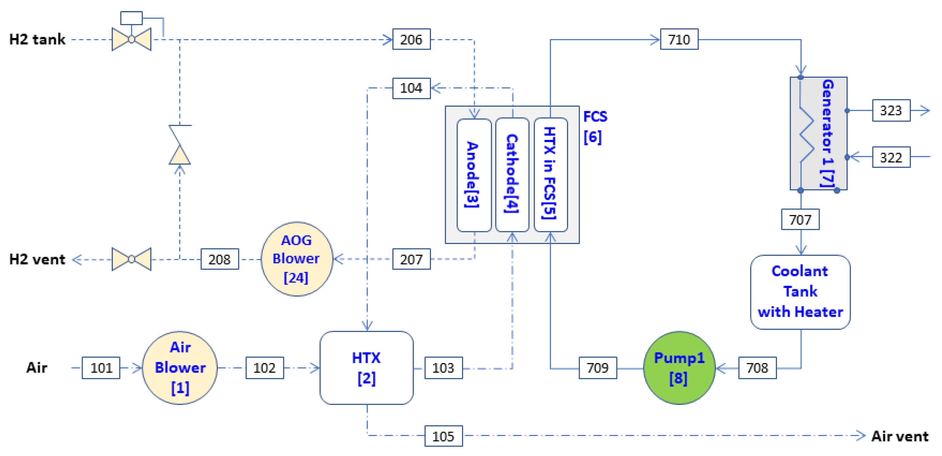
A schematic of a 5-kW HT-PEMFC system is shown in Figure 1. The system consists of eight components: air blower (1), heat exchanger (HTX) (2), anode (3), cathode (4), HTX) in fuel cell stack (FCS) (5), FCS (6), generator (7), and pump 1 (8). The FCS is an artificial component that produces electrical work and generates heat by consuming fuel (chemical exergy) without considering the mass flow in it. The mass flow and the physical exergies of fuel were considered in the anode [17]. The generator serves to provide heat to the LiBr–water ARS.

Table 1. Property values and thermal, and mechanical exergy flows and entropy flow rates at various state points in hydrogen-fueled 5-kW PEMFC.

States	$\dot{\mathit{m}}$ (kg/h)	$\mathit{T}$ (K)	$\mathit{P}$ (kPa)	$\dot{\mathit{H}}$ (kJ/h)	$\dot{\mathit{S}}$ (kJ/h-K)	${\dot{\mathit{E}}}_{\mathit{x}}$ (kJ/h)
101	14.15	299.3	101.05	16.89	2.71	−5.09
102	14.15	312.1	111.22	199.09	2.92	115.55
103	14.04	363.2	104.54	930.39	5.34	124.83
104	14.42	433.2	100.85	2428.72	10.32	287.61
105	14.42	300.5	101.37	41.69	3.73	−131.45
206	0.3960	300.0	103.30	10.37	0.035	0.006
207	0.0169	433.2	101.34	32.70	0.091	0.048
707	1013.0	413.2	101.11	345,048.1	804.0	‘-------’
708	1013.0	410.2	101.13	337,654.2	786.0	‘--------’
709	1013.0	410.2	158.00	337,752.8	786.3	‘-------’
710	1013.0	423.2	125.11	369,694.4	863.0	‘-------’

shows the measured values of the mass flow rate, temperature, and pressure, which are provided by the Fuel Cell Research Center, Korea Institute of Energy Research, and the calculated values of the enthalpy, entropy and exergy flow rate at various state points of the HT-PEMFC system based on the measured data.

3.1. Exergy-Balance Equation for the HT-PEMFC System

The following exergy-balance equations can be obtained by applying the general exergy-balance equation given in Equation (3) to each component in the 5-kW HT-PEMFC system. The first digit in the subscript indicates a specific fluid stream; 1 for air, 2 for hydrogen, 3 for the LiBr–water solution and 7 for coolant fluid. The second and third digits denote a digital number that represents the inlet or outlet state points in components. The number in the bracket indicates each component. The anode off gas (AOG) blower and coolant tank were considered to be parts of the anode and generator, respectively:

1.

Air Blower {1}:

$$\begin{array}{l}({\dot{E}}_{x,101}^T-{\dot{E}}_{x,102}^T)+({\dot{E}}_{x,101}^P-{\dot{E}}_{x,102}^P)+({\dot{E}}_{x,101}^C-{\dot{E}}_{x,102}^C)\\ +T_0({\dot{S}}_{101}-{\dot{S}}_{102}+\frac{{\dot{Q}}_{\left\{1\right\}}}{T_0})={\dot{E}}_{x,\left\{1\right\}}^W\end{array}$$

(13)

In Equation (13), the superscript C means chemical exergy of air.

2.

HTX {2}:

$$\begin{array}{l}\left[({\dot{E}}_{x,102}^T-{\dot{E}}_{x,103}^T)+({\dot{E}}_{x,104}^T-{\dot{E}}_{x,105}^T)\right]+\left[({\dot{E}}_{x,102}^P-{\dot{E}}_{x,103}^P)+({\dot{E}}_{x,104}^P-{\dot{E}}_{x,105}^P)\right]\\ +\left[({\dot{E}}_{x,102}^C-{\dot{E}}_{x,103}^C)+({\dot{E}}_{x,104}^C-{\dot{E}}_{x,105}^C)\right]+T_0\left({\dot{S}}_{102}-{\dot{S}}_{103}+{\dot{S}}_{104}-{\dot{S}}_{105}+\frac{{\dot{Q}}_{\left\{2\right\}}}{T_0}\right)=0\end{array}$$

(14)

3.

Anode {3} + AOG Blower {24}:

$$({\dot{E}}_{x,206}^T-{\dot{E}}_{x,208}^T)+({\dot{E}}_{x,206}^P-{\dot{E}}_{x,208}^P)+T_0\left({\dot{S}}_{206}-{\dot{S}}_{208}+\frac{{\dot{Q}}_{\left\{3\right\}}}{T_0}\right)={\dot{E}}_{x,\left\{24\right\}}^W$$

(15)

4.

Cathode {4}:

$$({\dot{E}}_{x,103}^T-{\dot{E}}_{x,104}^T)+({\dot{E}}_{x,103}^P-{\dot{E}}_{x,104}^P)+({\dot{E}}_{x,103}^C-{\dot{E}}_{x,104}^C)+T_0\left({\dot{S}}_{103}-{\dot{S}}_{104}+\frac{{\dot{Q}}_{\left\{4\right\}}}{T_0}\right)=0$$

(16)

5.

HTX in FCS {5}:

$$({\dot{E}}_{x,709}^T-{\dot{E}}_{x,710}^T)+({\dot{E}}_{x,709}^P-{\dot{E}}_{x,710}^P)+T_0\left({\dot{S}}_{709}-{\dot{S}}_{710}+\frac{{\dot{Q}}_{\left\{5\right\}}}{T_0}\right)=0$$

(17)

6.

FCS {6}:

$${\dot{E}}_x^{CHE}+{\dot{E}}_{x,\left\{6\right\}}^T-T_0{\dot{S}}_{gen,\left\{6\right\}}={\dot{E}}_{x,\left\{6\right\}}^W$$

(18)

where $E_{x,\left\{6\right\}}^T=E_{x,\left\{6\right\}}^{CHE}-E_{x,\left\{6\right\}}^W-T_o{\dot{S}}_{gen,\left\{6\right\}}$.

7.

Generator {7} + Coolant tank:

$$({\dot{E}}_{x,710}^{DT}-{\dot{E}}_{x,708}^{DT})+({\dot{E}}_{x,710}^P-{\dot{E}}_{x,708}^P)+{\dot{Q}}_{in}+T_0\left({\dot{S}}_{710}-{\dot{S}}_{708}+\frac{{\dot{Q}}_{\left\{7\right\}}}{T_0}\right)=0$$

(19)

8.

Pump 1 {8}:

$$({\dot{E}}_{x,708}^{DT}-{\dot{E}}_{x,709}^{DT})+({\dot{E}}_{x,708}^P-{\dot{E}}_{x,709}^P)+T_0\left({\dot{S}}_{708}-{\dot{S}}_{709}+\frac{{\dot{Q}}_{\left\{8\right\}}}{T_0}\right)={\dot{E}}_{\left\{8\right\}}^W$$

(20)

The chemical exergy of air in Equation (13) can be described as [14]:

$$e^{CHE}=R{T}_o\left[\ln (\frac{1+{\tilde{\omega }}_o}{1+\tilde{\omega }})+\frac{\tilde{\omega }}{1+\tilde{\omega }}\ln (\frac{\tilde{\omega }}{{\tilde{\omega }}_o})\right]$$

(21)

where $\tilde{\omega }=1.608 \omega$, $\omega$ is the absolute humidity and $\tilde{\omega }$ is the molar ratio of water vapor to dry air in air.

3.2. Cost-Balance Equations for the HT-PEMFC System

The equations for the exergy cost-balance equation given in Equation (10) for each device of HT-PEMFC shown in Figure 1 are as follows. In the cost-balance equation, a new unit cost may be assigned to the unit cost of the product representing the characteristics of the device. For example, since an air blower is a device that increases the pressure of air, a new unit cost of C1P is given to the mechanical exergy of air, and it is expressed in gothic style:

1.

Air Blower {1}:

$$\begin{array}{c}({\dot{E}}_{x,101}^T-{\dot{E}}_{x,102}^T)C_T+({\dot{E}}_{x,101}^P-{\dot{E}}_{x,102}^P){\mathit{C}}_{\mathbf{1}\mathit{P}}+({\dot{E}}_{x,101}^C-{\dot{E}}_{x,102}^C)C_C\\ +T_0\left({\dot{S}}_{101}-{\dot{S}}_{102}+\frac{{\dot{Q}}_{\left\{1\right\}}}{T_0}\right)C_S+{\dot{Z}}_{\left\{1\right\}}={\dot{E}}_{x,\left\{1\right\}}^W{C}_W\end{array}$$

(22)

2.

HTX {2}:

$$\begin{array}{l}\left[({\dot{E}}_{x,102}^T-{\dot{E}}_{x,103}^T)+({\dot{E}}_{x,104}^T-{\dot{E}}_{x,105}^T)\right]{\mathit{C}}_{\mathbf{2}\mathit{T}}+\left[({\dot{E}}_{x,102}^P-{\dot{E}}_{x,103}^P)+({\dot{E}}_{x,104}^P-{\dot{E}}_{x,105}^P)\right]C_P\\ \left[({\dot{E}}_{x,102}^C-{\dot{E}}_{x,103}^C)+({\dot{E}}_{x,104}^C-{\dot{E}}_{x,105}^C)\right]C_C+T_0\left({\dot{S}}_{102}-{\dot{S}}_{103}+{\dot{S}}_{104}-{\dot{S}}_{105}+\frac{{\dot{Q}}_{\left\{2\right\}}}{T_0}\right)C_S\\ +{\dot{Z}}_{\left\{2\right\}}=0\end{array}$$

(23)

3.

Anode {3} + AOG Blower {24}:

$$({\dot{E}}_{x,206}^T-{\dot{E}}_{x,208}^T){\mathit{C}}_{\mathbf{3}\mathit{T}}+({\dot{E}}_{x,206}^P-{\dot{E}}_{x,208}^P)C_P+T_0\left({\dot{S}}_{206}-{\dot{S}}_{208}+\frac{{\dot{Q}}_{\left\{3\right\}}}{T_0}\right)C_S+{\dot{Z}}_{\left\{3\right\}}={\dot{E}}_{x,\left\{3\right\}}^W{C}_W$$

(24)

4.

Cathode {4}:

$$\begin{array}{c}({\dot{E}}_{x,103}^T-{\dot{E}}_{x,104}^T)C_T+({\dot{E}}_{x,103}^P-{\dot{E}}_{x,104}^P)C_P+({\dot{E}}_{x,103}^C-{\dot{E}}_{x,104}^C){\mathit{C}}_{\mathbf{4}\mathit{C}}\\ +T_0\left({\dot{S}}_{103}-{\dot{S}}_{104}+\frac{{\dot{Q}}_{\left\{4\right\}}}{T_0}\right)C_S+{\dot{Z}}_{\left\{4\right\}}=0\end{array}$$

(25)

5.

HTX in FCS {5}:

$$({\dot{E}}_{x,709}^{DT}-{\dot{E}}_{x,710}^{DT}){\mathit{C}}_{\mathbf{5}D\mathit{T}}+({\dot{E}}_{x,709}^P-{\dot{E}}_{x,710}^P)C_P+T_0\left({\dot{S}}_{709}-{\dot{S}}_{710}+\frac{{\dot{Q}}_{\left\{5\right\}}}{T_0}\right)C_S+{\dot{Z}}_{\left\{5\right\}}=0$$

(26)

6.

FCS {6}:

$${\dot{E}}_x^{CHE}{C}_o+{\dot{E}}_{x,\left\{6\right\}}^T{C}_T-T_0{\dot{S}}_{gen,\left\{6\right\}}{C}_S+{\dot{Z}}_{\left\{6\right\}}={\dot{E}}_{x,\left\{6\right\}}^W{\mathit{C}}_{\mathbf{6}\mathit{W}}$$

(27)

7.

Generator {7}:

$$({\dot{E}}_{x,710}^{DT}-{\dot{E}}_{x,708}^{DT}){\mathit{C}}_{\mathbf{7}D\mathit{T}}+({\dot{E}}_{x,710}^P-{\dot{E}}_{x,708}^P)C_P+T_0\left({\dot{S}}_{710}-{\dot{S}}_{708}+\frac{{\dot{Q}}_{\left\{7\right\}}}{T_0}\right)C_S+{\dot{Z}}_{\left\{7\right\}}=0$$

(28)

8.

Pump 1 {8}:

$$({\dot{E}}_{x,708}^{DT}-{\dot{E}}_{x,709}^{DT})C_{DT}+({\dot{E}}_{x,708}^P-{\dot{E}}_{x,709}^P){\mathit{C}}_{\mathbf{8}\mathit{P}}+T_0\left({\dot{S}}_{708}-{\dot{S}}_{709}+\frac{{\dot{Q}}_{\left\{8\right\}}}{T_0}\right)C_S+{\dot{Z}}_{\left\{8\right\}}={\dot{E}}_{\left\{8\right\}}^W{C}_W$$

(29)

As can be seen above, eight cost-balance equations were obtained from eight components. However, there are 14 unknowns in the cost balance equations described above: C_1P, C_2T, C_3T, C_4C, C_5DT, C_6W, C_7DT, C_8P, C_T, C_DT, C_P, C_C, C_W and C_S. Therefore, we need six more auxiliary equations to find the unknowns. The following six auxiliary equations can be obtained from the junction for thermal exergy of the gas and coolant fluid, mechanical exergy, chemical exergy, electrical exergy and the system boundary of exergy flows.

Thermal exergy junction for the gas stream:

$$\begin{array}{l}\left[({\dot{E}}_{x,102}^T-{\dot{E}}_{x,103}^T)+({\dot{E}}_{x,104}^T-{\dot{E}}_{x,105}^T)+({\dot{E}}_{x,206}^T-{\dot{E}}_{x,207}^T)\right]{\mathit{C}}_{\mathit{T}}\\ =\left[({\dot{E}}_{x,102}^T-{\dot{E}}_{x,103}^T)+({\dot{E}}_{x,104}^T-{\dot{E}}_{x,105}^T)\right]C_{2\mathrm{T}}+({\dot{E}}_{x,206}^T-{\dot{E}}_{x,207}^T)C_{3\mathrm{T}}\end{array}$$

(30)

Mechanical exergy junction for the gas stream:

$$\begin{array}{l}\left[({\dot{E}}_{x,101}^P-{\dot{E}}_{x,102}^P)+({\dot{E}}_{x,708}^P-{\dot{E}}_{x,709}^P)\right]{\mathit{C}}_{\mathit{P}}=\\ ({\dot{E}}_{x,101}^P-{\dot{E}}_{x,102}^P)C_{1\mathrm{P}}+({\dot{E}}_{x,708}^P-{\dot{E}}_{x,709}^P)C_{8\mathrm{P}}\end{array}$$

(31)

Thermal exergy junction of the coolant:

$$\begin{array}{l}\left[({\dot{E}}_{x,709}^{DT}-{\dot{E}}_{x,710}^{DT})+({\dot{E}}_{x,710}^{DT}-{\dot{E}}_{x,708}^{DT})\right]{\mathit{C}}_{D\mathit{T}}\\ =({\dot{E}}_{x,709}^{DT}-{\dot{E}}_{x,710}^{DT})C_{5\mathrm{DT}}+({\dot{E}}_{x,710}^{DT}-{\dot{E}}_{x,708}^{DT})C_{7\mathrm{DT}}\end{array}$$

(32)

Electricity junction:

$${\dot{E}}_{x,\left\{6\right\}}^W{\mathit{C}}_{\mathit{W}}={\dot{E}}_{x,\left\{6\right\}}^W{C}_{6\mathrm{W}}$$

(33)

Chemical exergy junction:

$$({\dot{E}}_{x,104}^C-{\dot{E}}_{x,105}^C){\mathit{C}}_C=({\dot{E}}_{x,104}^C-{\dot{E}}_{x,105}^C)C_{4C}$$

(34)

System boundary:

$$\begin{array}{l}({\dot{E}}_{x,105}^T-{\dot{E}}_{x,101}^T)C_T+({\dot{E}}_{x,105}^P-{\dot{E}}_{x,101}^P)C_P+({\dot{E}}_{x,105}^C-{\dot{E}}_{x,101}^C)C_C\\ +T_0\left({\dot{S}}_{105}-{\dot{S}}_{101}+{{\displaystyle \sum }}^{}\frac{{\dot{Q}}_{\left\{i\right\}}}{T_0}\right){\mathit{C}}_{\mathit{S}}=0\end{array}$$

(35)

Using Equations (30) to (35) and adding Equations (22) to (29), we obtain the following equation, which is the cost-balance equation for the entire system:

$${\dot{E}}_x^{CHE}{C}_o+{\displaystyle \sum }_{i=1}^8{\dot{Z}}_i={\dot{E}}_{x,net}^W{C}_W$$

(36)

One may obtain the unit cost of electricity produced by HT-PEMFC system using Equation (36).

4. Double-Effect LiBr–Water Absorption Refrigeration Systems

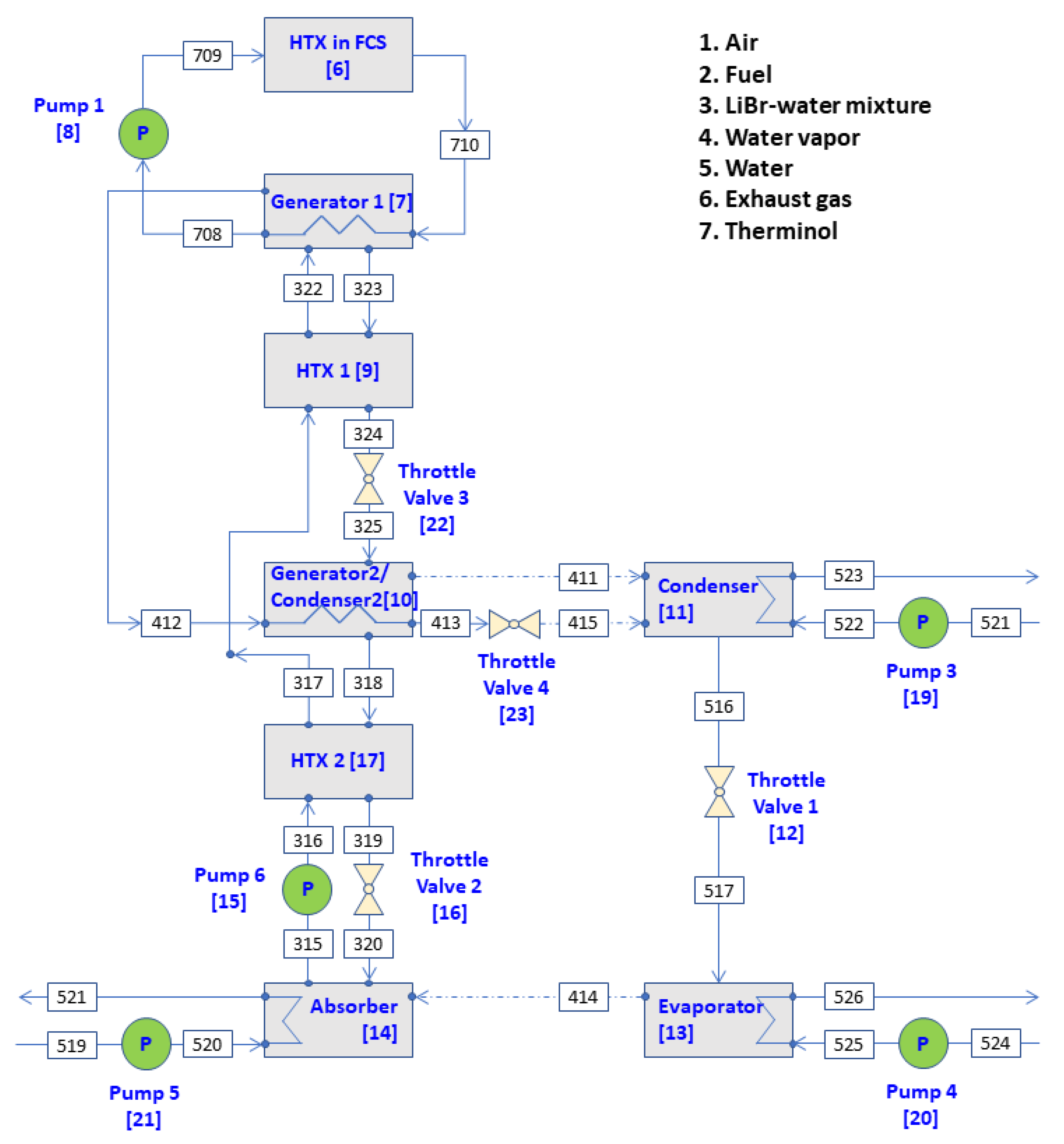
In this study, two types of dual-effect LiBr–water ARSs that can be operated in conjunction with a 5-kW HT-PEMFC were considered. One of them is an industrial double effect ARS which uses generator 2/condenser 2, where the condensation and evaporation of the refrigerant take place, as shown in Figure 2.

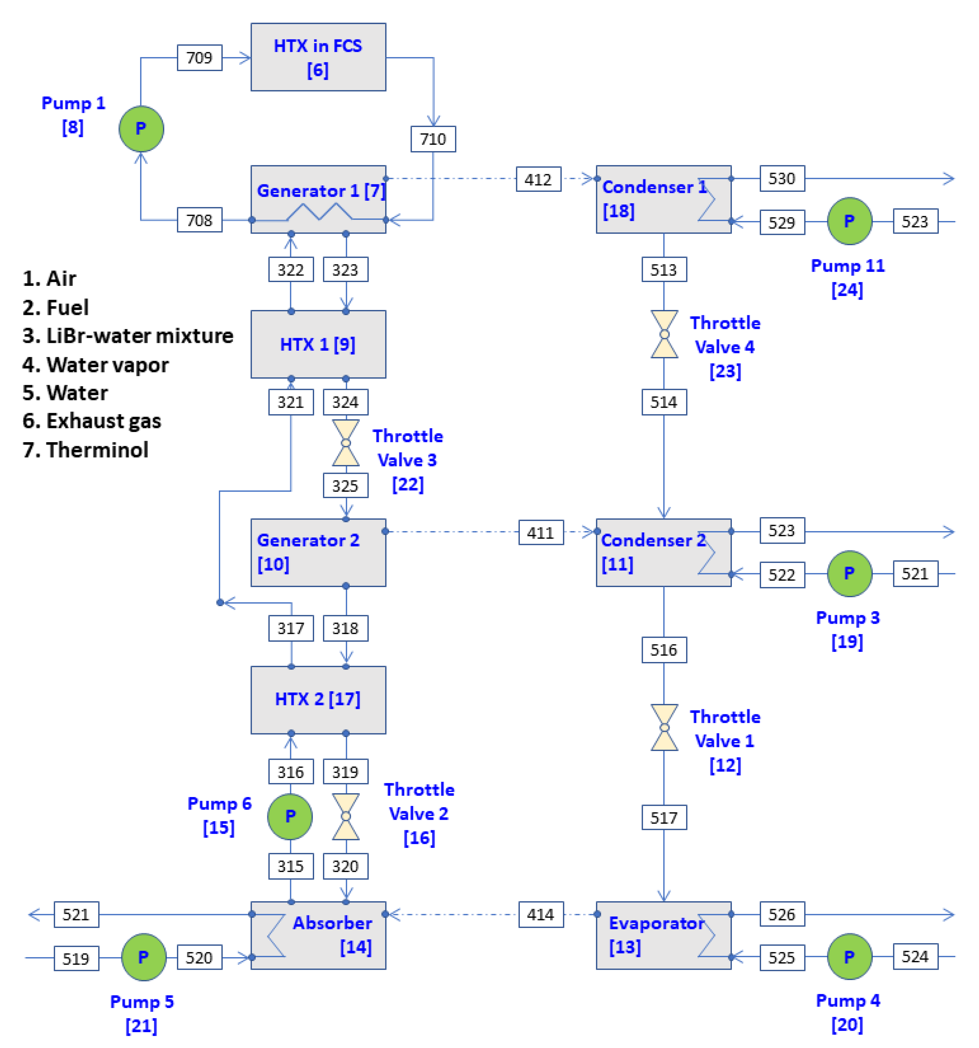
That is, the primary vapor refrigerant (412) from the high-pressure generator 1 is condensed in the generator 2/condenser 2 to form condensate, which enters condenser (415) through a throttle valve. The secondary vapor refrigerant (411) forms in the generator 2/condenser 2 using the latent heat generated during the condensation of the primary vapor refrigerant and the heat input of LiBr–water solution from the high-temperature generator 1. The advantage of this industrial double effect ARS is that more vapor refrigerant can be produced in the generator 2/condenser 2, which consequently reduce the heat required for vapor refrigerant production in the generator 1. This refrigeration system is composed of eight units: generator 1 {7}, condenser {11}, HTX 1 {9}, generator 2/condenser 2 {10}, HTX 2 {17}, pump 6 {15}, absorber {14} and evaporator {13}. The other ARS is the series double-effect LiBr–water ARS shown in Figure 3. Another condenser (condenser 1) is installed in this double effect ARS. The primary vapor refrigerant generated in generator 1 is sent to condenser 1 instead of generator 2. In this refrigeration system, the heat input for generating the secondary vapor refrigerant 411 comes from the hot LiBr–water solution only from generator 1.

4.1. Analysis of the Double Effect LiBr–Water Absorption Refrigeration System

Analysis of the double-effect LiBr–water ARS can be performed by pre-assuming the cooling load of the evaporator and the operating temperatures of generator 1 ($T_{gen1}$), generator 2/condenser 2 ($T_{gencon}$), the condenser ($T_{con}$), the evaporator ($T_{eva}$) and the absorber ($T_{abs}$). Analyses can be performed sequentially from the evaporator {8} as follows. The physical properties of LiBr–water solutions such as enthalpy and entropy were obtained from Kaita [18].

Evaporator {13}:

The cooling load in the evaporator can be obtained by adjusting the outlet temperature when the inlet temperature of the chilled water is given as follows:

$${\dot{Q}}_{chil}={\dot{m}}_{525}(h_{526}-h_{525})$$

(37)

Given the cooling load, the mass flow rate of water vapor, which is the refrigerant leaving the evaporator, can be calculated as:

$${\dot{m}}_{414}=\left|{\dot{Q}}_{chil}\right|/(h_{414}-h_{517})$$

(38)

The first law of thermodynamics for the evaporator is given by:

$${\dot{Q}}_{eva}={\dot{m}}_{414}(h_{414}-h_{517})+{\dot{Q}}_{chil}+E_{x,eva}^W$$

(39)

The pressures at state points 414 (evaporator) and 516 (condenser) are the saturated vapor pressures of water corresponding to the operating temperatures of the evaporator and condenser, respectively. The three pressure levels in the refrigeration system, the saturation pressure of the LiBr–water solution in the generator 1 ($P_{323}$ = $P_{322}$), generator 2/condenser 2 pressure ($P_{325}$ = $P_{318}$) and the absorber pressure were obtained using a Duhring diagram [19].

Absorber {14}:

The mass flow rates of the LiBr–Water solution entering (320) and leaving (315) the absorber can be obtained under the condition that the mass flow rates of LiBr entering and leaving the absorber are the same. In other words, the cooling load in the evaporator can be obtained by adjusting the outlet temperature when the inlet temperature of the chilled water is given as follows:

$${\dot{m}}_{315}\cdot X_{315}={\dot{m}}_{320}\cdot X_{320}={\dot{m}}_{319}\cdot X_{319}={\dot{m}}_{318}\cdot X_{318}$$

(40)

In Equation (40), X is the concentration of LiBr (% kg of LiBr in the solution).

Using Equation (40) and the mass conservation equation in the absorber, the mass flow rates of the LiBr–water solution at state points 315 and 318 are given as follows:

$${\dot{m}}_{315}={\dot{m}}_{316}={\dot{m}}_{317}=\frac{{\dot{m}}_{414}\cdot X_{318}}{X_{318}-X_{315}}$$

(41)

$${\dot{m}}_{320}={\dot{m}}_{319}={\dot{m}}_{318}=\frac{{\dot{m}}_{414}\cdot X_{315}}{X_{318}-X_{315}}$$

(42)

When the concentration of LiBr is in the range of 0.50 to 0.65, the following equation [20] approximately holds between the temperature of the refrigerant, $t_R$; the saturation temperature of the LiBr–water solution, t_m; and the concentration of LiBr, X:

$$t_R=49.04-135.65\cdot (1.125-0.47X)t_m$$

(43)

Using Equation (43), the concentration of LiBr–water solution at state points 315 and 318 can be obtained as follows:

$$X_{315}=\frac{49.04+1.125\cdot t_{315}-t_{414}}{134.65+0.47\cdot t_{315}}$$

(44)

$$X_{318}=\frac{49.04+1.125\cdot t_{411}-t_{516}}{134.65+0.47\cdot t_{411}}$$

(45)

The first law of thermodynamics for the absorber is as follows:

$${\dot{Q}}_{abs}={\dot{m}}_{325}{h}_{325}-{\dot{m}}_{320}{h}_{320}-{\dot{m}}_{414}{h}_{414}+{\dot{m}}_{520}(h_{521}-h_{520})+{\dot{E}}_{x,abc}^W$$

(46)

Pump 6 {15}:

The temperature of the LiBr–water solution after passing through the pump hardly changes. The work required for the pump can be calculated by the following equation:

$${\dot{W}}_{pump}={\dot{m}}_{315}\cdot (P_{315}-P_{316})v_{315}$$

(47)

where ${\nu }_{315}$ in Equation (47) is the specific volume of the LiBr–water solution at state point 315.

Throttle valve 2 {16}:

The enthalpy of the LiBr–water solution does not change after passing through the throttle valve, so there is no temperature change at state points 319 and 320. However, there is a pressure difference between these two state points, so there will be a change in entropy, but there is currently no way to calculate it. In this study, it was assumed that there would be almost no change in entropy in the throttle valve, and no lost work was considered in the throttle valve.

HTX 2 {17}:

The effectiveness of the HTX 2 can be defined by the following equation.

$${\epsilon }_{HTX2}=\frac{h(318)-h(319)}{h(318)-h(316)}\approx \frac{t_{318}-t_{319}}{t_{318}-t_{316}}$$

(48)

Knowing the effectiveness of HTX 2, the temperature at the state point 319, one of the outlet temperatures in HTX 2, can be obtained as follows:

$$t_{319}=t_{318}-{\epsilon }_{HTX1}(t_{318}-t_{315})$$

(49)

The conservation of energy for HTX 2 is given by:

$${\dot{m}}_{316}{C}_{p,316}(t_{317}-t_{316})={\dot{m}}_{318}{C}_{p,318}(t_{318}-t_{319})$$

(50)

$C_p$ in Equation (50) is the heat capacity of the LiBr–water solution:

$$t_{317}=t_{316}+\frac{{\dot{m}}_{318}{C}_{p,318}{\epsilon }_{HTX1}(t_{318}-t_{315})}{{\dot{m}}_{316}{C}_{p,315}}$$

(51)

Generator 1 {7}:

The conservation of mass for Generator 1 is given by:

$${\dot{m}}_{322}={\dot{m}}_{323}+{\dot{m}}_{412}$$

(52)

If the mass flow rate of the refrigerant leaving state point 412 is $f$ times the refrigerant required in the condenser, we have:

$${\dot{m}}_{412}=f\cdot {\dot{m}}_{414} (=f\cdot {\dot{m}}_{516})$$

(53)

where $f$ in Equation (53) is a number less than 1.

The mass flow rate of LiBr entering and exiting generator 1 must be the same, so the following equation holds:

$${\dot{m}}_{322}{X}_{322}={\dot{m}}_{323}{X}_{323}={\dot{m}}_{317}{X}_{317}$$

(54)

From Equations (52) and (54), we obtain:

$$X_{323}=\frac{{\dot{m}}_{317}{X}_{317}}{{\dot{m}}_{323}}=\frac{{\dot{m}}_{317}{X}_{317}}{{\dot{m}}_{317}-{\dot{m}}_{412}}$$

(55)

The heat received by the LiBr–water solution in generator 1 from the thermal fluid coming out of the stack is given by:

$${\dot{Q}}_{gen1}={\dot{m}}_{323}{h}_{323}-{\dot{m}}_{322}{h}_{322}+{\dot{m}}_{412}{h}_{412}$$

(56)

HTX 1 {9}:

The effectiveness of the HTX 1 can be written as:

$${\epsilon }_{HTX1}\approx \frac{t_{323}-t_{324}}{t_{323}-t_{317}}$$

(57)

From Equation (57), the temperature for state point 324 can be obtained:

$$t_{324}=t_{323}-{\epsilon }_{HTX1}(t_{323}-t_{317})$$

(58)

The energy conservation for HTX 1 can be written as:

$$\begin{array}{ll}{\dot{m}}_{317}{C}_{p,317}(t_{322}-t_{317})& ={\dot{m}}_{323}{C}_{p,323}(t_{323}-t_{324})\\ & ={\dot{m}}_{323}{C}_{p,323}{\epsilon }_{HTX1}(t_{323}-t_{317})\end{array}$$

(59)

From Equation (59), the temperature at state point 323 can be obtained as follows:

$$t_{322}=t_{317}+\frac{{\dot{m}}_{323}{C}_{p,323}{\epsilon }_{HTX1}(t_{323}-t_{317})}{{\dot{m}}_{317}{C}_{p,317}}$$

(60)

Generator 2/Condenser 2 {10}:

The conservation of mass and energy equations of generator 2/condenser 2 are given as follows:

$${\dot{m}}_{325}={\dot{m}}_{318}+{\dot{m}}_{411}$$

(61)

$${\dot{m}}_{325}{C}_{p,325}{t}_{325}={\dot{m}}_{318}{C}_{p,318}{t}_{318}+{\dot{m}}_{411}{h}_{411}-{\dot{m}}_{412}(h_{412}-h_{413})$$

(62)

The mass flow rate at state point 414 is the sum of the mass flow rate at state point 412 and the mass flow rate at state point 411. So, we obtain the following relationship:

$${\dot{m}}_{411}=(1-f)\cdot {\dot{m}}_{414}$$

(63)

The temperature at state point 413 is considered to be the same as that of state point 411.

Condenser {11}:

The amount of heat lost by the refrigerant in the condenser is equal to the heat gained by the coolant. This is expressed as:

$$\begin{array}{ll}{\dot{Q}}_{con}& ={\dot{m}}_{414}\left[f(h_{415}-h_{516})+(1-f)(h_{411}-h_{516})\right]\\ & ={\dot{ m}}_{520}(h_{523}-h_{522})\end{array}$$

(64)

As above, if the cooling capacity of the evaporator and the temperature of the solution and refrigerant at the inlet and outlet of each unit are known, the calculation proceeds in the order of evaporator, absorber, pump 6, HTX 2, and generator 1, HTX 1, generator 2/condenser 2, and condenser. These results are considered reasonable if the estimated amount of heat input to the generator to produce the desired cooling capacity is approximately equal to the heat supply by the FCS in the HT-PEMFC system.

4.2. Exergy-Balance Equations for LiBr–Water Absorption Refrigeration System

In the case of a refrigeration system, since the change in the mechanical exergy in the exergy flow is relatively small compared to the thermal exergy, it is convenient to separate the exergy stream according to the type of material flow rather than separating it into thermal exergy and mechanical exergy [12]. In the ARS, the analysis was performed by separating the material stream into the LiBr–water solution (rs), refrigerant steam or water (rf) and cooling water (wa). In addition, with exception of pump 6 of the LiBr–water solution, pumps for the flow of coolant for heat exchange in the evaporator, absorber and condenser were included in the respective equipment. An example of an exergy analysis for the evaporator is:

Evaporator {13}:

$$({\dot{E}}_{x,517}^{rf}-{\dot{E}}_{x,414}^{rf})+{\dot{Q}}_{chil}+(-{\dot{E}}_{x,\left\{13\right\}}^D)=0$$

(65)

Pump 4 {20}:

$$({\dot{E}}_{x,524}^{wa}-{\dot{E}}_{x,525}^{wa})-{\dot{E}}_{x,\left\{20\right\}}^D={\dot{E}}_{x,\left\{20\right\}}^W$$

(66)

where the ${\dot{E}}_x^D$ variables in Equations (65) and (66) mean the rate of lost work in the components and are defined in Equation (4). By summing Equations (65) and (66), we obtain an exergy-balance equation for the evaporator and pump 4:

$$({\dot{E}}_{x,517}^{rf}-{\dot{E}}_{x,414}^{rf})+({\dot{E}}_{x,524}^{wa}-{\dot{E}}_{x,525}^{wa})+{\dot{Q}}_{chil}+(-{\dot{E}}_{x,eva}^D)={\dot{E}}_{x,\left\{20\right\}}^W$$

(67)

where ${\dot{E}}_{x,eva}^D={\dot{E}}_{x,\left\{13\right\}}^D+{\dot{E}}_{x,\left\{20\right\}}^D$.

As can be seen from Equation (69), the cooling capacity acts as a “heat sink”.

The exergy balance equations for the absorber, pump 6, HTX 2, generator 1, HTX 1, generator 2/condenser 2 and condenser can be obtained in the same way as deriving the exergy balance equation for the evaporator as follows:

Absorber {14} + pump 5 {21}:

$$({\dot{E}}_{x,320}^{rs}-{\dot{E}}_{x,315}^{rs})+{\dot{E}}_{x,414}^{rf}+({\dot{E}}_{x,519}^{wa}-{\dot{E}}_{x,521}^{wa})-{\dot{E}}_{x,abs}^D={\dot{E}}_{x,\left\{21\right\}}^W$$

(68)

Pump 6 {15}:

$$({\dot{E}}_{x,315}^{rs}-{\dot{E}}_{x,316}^{rs})-{\dot{E}}_{x,pump6}^D={\dot{E}}_{x,\left\{15\right\}}^W$$

(69)

HTX 2 {17}:

$$({\dot{E}}_{x,323}^{rs}-{\dot{E}}_{x,324}^{rs})+({\dot{E}}_{x,317}^{rs}-{\dot{E}}_{x,322}^{rs})-{\dot{E}}_{x,htx1}^D=0$$

(70)

Generator 1 {7}:

$$({\dot{E}}_{x,322}^{rs}-{\dot{E}}_{x,323}^{rs})-{\dot{E}}_{x,412}^{rf}+({\dot{E}}_{x,710}^{cool}-{\dot{E}}_{x,708}^{cool})+{\dot{Q}}_{gen1}+(-{\dot{E}}_{x,gen1}^D)=0$$

(71)

The heat input in generator 1 acts as “heat source”.

HTX 1 {9}:

$$({\dot{E}}_{x,323}^{rs}-{\dot{E}}_{x,324}^{rs})+({\dot{E}}_{x,317}^{rs}-{\dot{E}}_{x,322}^{rs})-{\dot{E}}_{x,htx1}^D)=0$$

(72)

Generator 2/Condenser 2 {10}:

$$({\dot{E}}_{x,325}^{rs}-{\dot{E}}_{x,318}^{rs})+({\dot{E}}_{x,412}^{rf}-{\dot{E}}_{x,413}^{rf}-{\dot{E}}_{x,411}^{rf})-{\dot{E}}_{x,gencon}^D=0$$

(73)

Condenser {11} + pump 3 {19}:

$$({\dot{E}}_{x,411}^{rf}+{\dot{E}}_{x,415}^{rf}-{\dot{E}}_{x,516}^{rf})+({\dot{E}}_{x,521}^{wa}-{\dot{E}}_{x,523}^{wa})-{\dot{E}}_{x,con}^D={\dot{E}}_{x,\left\{19\right\}}^W$$

(74)

4.3. Cost-Balance Equations for LiBr–Water Absorption Refrigeration System

As described above for the industrial double-effect ARS, eight exergy-balance equations were obtained for the main devices in Equations (67)–(74). Furthermore, there is one more exergy-balance equation for the “boundary” of the system, so we can obtain nine exergy-balance equations for the refrigeration system. A unit cost is assigned for each type of exergy stream to these nine exergy-balance equations. That is, a unit cost of $C_{rs}$, $C_{rf}$ and $C_{wa}$ is assigned to the LiBr–water solution, refrigerant and cooling water flows, respectively, and the unit cost of C_S and Cchil are assigned to the lost work rate and chilled water, respectively. Thus, we have nine cost-balance equations out nine 9 exergy-balance equations. However, although there are five unknowns we are looking for, there are more equations to be solved than unknowns, so we cannot find a unique solution. In this case, it is better to combine the devices in the system to obtain four exergy-balance equations and corresponding exergy cost-balance equations as follows:

Evaporator {13} + pump 4 {20}:

$$({\dot{E}}_{x,517}^{rf}-{\dot{E}}_{x,414}^{rf})C_{rf}+{\dot{Q}}_{chil}{C}_{chil}+(-{\dot{E}}_{x,eva}^D-{\dot{Q}}_{chil})C_S+\left[({\dot{Z}}_{\left\{13\right\}}+{\dot{Z}}_{\left\{20\right\}})-{\dot{E}}_{x,\left\{20\right\}}^W{C}_W\right]=0$$

(75)

Absorber {14} + pump 5 {21} + Pump 6 {15} + HTX 2 {17}:

$$\begin{array}{c}({\dot{E}}_{x,318}^{rs}-{\dot{E}}_{x,317}^{rs})C_{rs}+{\dot{E}}_{x,414}^{rf}{C}_{rf}+({\dot{E}}_{x,519}^{wa}-{\dot{E}}_{x,521}^{wa})C_{wa}-({\dot{E}}_{x,abs}^D+{\dot{E}}_{x,pump6}^D+{\dot{E}}_{x,htx2}^D)C_S\\ +\left[({\dot{Z}}_{\left\{14\right\}}+{\dot{Z}}_{\left\{15\right\}}+{\dot{Z}}_{\left\{17\right\}})-({\dot{E}}_{x,\left\{15\right\}}^W+{\dot{E}}_{x,\left\{21\right\}}^W)C_W\right]=0\end{array}$$

(76)

Generator 1 {7} + HTX 1 {9} + Generator 2/Condenser 2 {10}:

$$\begin{array}{c}({\dot{E}}_{x,317}^{rs}-{\dot{E}}_{x,318}^{rs})C_{rs}-{\dot{E}}_{x,411}^{rf}{C}_{rf}+{\dot{Q}}_{gen1}{C}_o-({\dot{E}}_{x,gen1}^D+{\dot{E}}_{x,htx1}^D+{\dot{E}}_{x,gencon}^D+{\dot{Q}}_{gen1})C_S\\ +({\dot{Z}}_{\left\{7\right\}}+{\dot{Z}}_{\left\{9\right\}}+{\dot{Z}}_{\left\{10\right\}})=0\end{array}$$

(77)

Condenser {11} + pump 3 {19}:

$$({\dot{E}}_{x,411}^{rf}+{\dot{E}}_{x,415}^{rf}-{\dot{E}}_{x,516}^{rf})C_{rf}+({\dot{E}}_{x,521}^{wa}-{\dot{E}}_{x,522}^{wa})C_{wa}-{\dot{E}}_{x,con}^D{C}_S+\left[{\dot{Z}}_{\left\{11\right\}}-{\dot{E}}_{x,\left\{19\right\}}^W{C}_W\right]=0$$

(78)

System boundary:

$$({\dot{E}}_{x,523}^{wa}-{\dot{E}}_{x,519}^{wa})C_{wa}-{{\displaystyle \sum }}^{}{\dot{E}}_{x,i}^D{C}_S=0$$

(79)

As clearly shown in Equations (76) and (78), the cost flow rate of the electricity consumed in the LiBr–water ARS was obtained using the unit cost of electricity of HT-PEMFC. As can be seen from Equations (75) and (77), the corresponding lost work for components with heat sources or sinks have been added to the cost balance equation.

In Equation (77), Co is the unit cost of heat produced by the PEMFC system, and it is taken as 0 because it is heat discarded by the PEMFC system. By solving the five equations from Equation (75) to Equation (79), the values of the unit costs such as $C_{rs}$, $C_{rf}$, $C_{wa}$, $C_S$ and $C_{chil}$ can be obtained. The unit cost of the chilled water for the refrigeration system can also be obtained from the following equation instead of solving the five cost-balance equations:

$$C_{chil}={{\displaystyle \sum }}^{}({\dot{Z}}_i-{\dot{E}}_{x,i}^W{C}_W)/\left|{\dot{Q}}_{chil}\right|$$

(80)

For the series double-effect LiBr–water ARS presented in Figure 3, the exergy-balance equation for generator 2 and condenser 1 and condenser 2 instead of generator 2/condenser 2 and condenser in the industrial double-effect ARS must be added to the exergy-balance equations given in Equations (67)–(74). These exergy-balance equations are as follows:

Generator 2 {10}:

$$({\dot{E}}_{x,325}^{rs}-{\dot{E}}_{x,318}^{rs})-{\dot{E}}_{x,411}^{rf}-{\dot{E}}_{x,gen2}^D=0$$

(81)

Condenser 1 {18} + pump 11 {24}:

$$({\dot{E}}_{x,412}^{rf}-{\dot{E}}_{x,513}^{rf})+({\dot{E}}_{x,523}^{wa}-{\dot{E}}_{x,530}^{wa})-{\dot{E}}_{x,con1}^D={\dot{E}}_{x,\left\{23\right\}}^W$$

(82)

Condenser 2 {11} + pump 3 {19}:

$$({\dot{E}}_{x,411}^{rf}-{\dot{E}}_{x,516}^{rf})+({\dot{E}}_{x,521}^{wa}-{\dot{E}}_{x,523}^{wa})-{\dot{E}}_{x,con1}^D={\dot{E}}_{x,\left\{19\right\}}^W$$

(83)

The exergy cost-balance equations for evaporator + pump 4 and absorber + pump 5 + pump 6 + heat exchanger 2 obtained from the ARS described above are used as is, but the cost-balance equations for generator 1 + heat exchanger 1 + generator 2, condenser 1 + condenser 2 and boundary must be rewritten. The new cost-balance equations for the parallel double-effect LiBr–water ARS are given as follows:

Generator 1 {7} + HTX 1 {9} + Generator 2 {10}:

$$\begin{array}{l}({\dot{E}}_{x,317}^{rs}-{\dot{E}}_{x,318}^{rs})C_{rs}-({\dot{E}}_{x,411}^{rf}+{\dot{E}}_{x,412}^{rf})C_{rf}+{\dot{Q}}_{gen1}{C}_o\\ -({\dot{E}}_{x,gen1}^D+{\dot{E}}_{x,htx1}^D+{\dot{E}}_{x,gen2}^D+{\dot{Q}}_{gen1})C_S+({\dot{Z}}_{\left\{7\right\}}+{\dot{Z}}_{\left\{9\right\}}+{\dot{Z}}_{\left\{10\right\}})=0\end{array}$$

(84)

Condenser 1 {18} + pump 11 {24} +condenser 2 {11} + pump 3 {19}:

$$\begin{array}{l}({\dot{E}}_{x,411}^{rf}+{\dot{E}}_{x,412}^{rf}-{\dot{E}}_{x,516}^{rf})C_{rf}+({\dot{E}}_{x,521}^{wa}-{\dot{E}}_{x,530}^{wa})C_{wa}-({\dot{E}}_{x,con1}^D+{\dot{E}}_{x,con2}^D)C_S\\ +\left[({\dot{Z}}_{\left\{11\right\}}+{\dot{Z}}_{\left\{18\right\}})-({\dot{E}}_{x,\left\{19\right\}}^W+{\dot{E}}_{x,\left\{23\right\}}^W)C_W\right]=0\end{array}$$

(85)

Boundary:

$$({\dot{E}}_{x,530}^{wa}-{\dot{E}}_{x,519}^{wa})C_{wa}-{{\displaystyle \sum }}^{}{\dot{E}}_{x,i}^D{C}_S=0$$

(86)

The unit cost of the cooling capacity of the series double-effect LiBr–water ARS can be obtained by solving Equations (75), (76) and (84)–(86):

5. Calculation Results and Discussion

As shown in Table 1, the measured mass flow rates of fuel (206) and air (101) entering this PEMFC system are 0.396 kg/h and 14.15 kg/h at full load, respectively. The number of cells in this PEMFC system is 160, the operating temperature is 160 °C and the current load at 6 kW power output is 63 A. Triethylene glycol was used as the fluid for cooling the stack, and the density and heat capacity of this cooling fluid are 1125.5 kg/m³ and 2.433 kJ/kg/K, respectively. The enthalpy and entropy of this cooling fluid were obtained using the equation for incompressible fluid. The maximum heat input to the high-pressure generator can be obtained from the difference in enthalpy flow rate between state points 707 and 710, which is approximately 24,640 kJ/h.

The exergy flow rates into and out of each component of the HT-PEMFC system are shown in

Table 2. Exergy balance for each component in hydrogen-fueled 5-kW PEMFC.

Component	Net Exergy Flow Rates (kJ/h)				Irreversibility Rate (kJ/h)
	${\dot{\mathit{E}}}_{\mathit{x}}^{\mathit{W}}$	${\dot{\mathit{E}}}_{\mathit{x}}^{\mathit{C}\mathit{H}\mathit{E}}$	${\dot{\mathit{E}}}_{\mathit{x}}^{\mathit{T}}$	${\dot{\mathit{E}}}_{\mathit{x}}^{\mathit{P}}$
Air blower	−133.057	0.0	4.490	116.157	12.411
HTX	0.0	0.0	−342.209	−67.569	409.778
Anode	0.0	0.0	9.420	−9.378	−0.042
Cathode	0.0	1039.233	207.394	−44.620	−1202.008
HTX in FCS	0.0	0.0	9083.807	−29.597	−9054.210
FCS	21,600.0	−45,474.085	71.623	0.0	23,802.462
Generator 1	0.0	0.0	−7072.115	−13.501	7085.615
Pump 1	−51.184	0.0	26.924	51.184	−26.924

. In the exergy flow, the negative sign is the exergy input to the device and the positive sign is the product exergy. In the exergy balance equation, the irreversibility due to entropy generation plays the role of product exergy. Approximately 45,474 kJ/h of fuel exergy per hour is fed into the FCS, producing 21,600 kJ/h (6 kW) of electricity per hour and 23,874 kJ/h of thermal energy per hour. This waste heat is energy that can be used as a heat source for absorption chillers in the generator.

Table 3. Initial investments, annualized costs and corresponding monetary flow rates of each component in hydrogen-fueled 5-kW PEMFC system.

Component	Initial Investment Cost (USD)	Annualized Cost (USD)	Monetary Flow Rate (USD/h)
Air blower	2947.6 (1740.8) 1	380.4	0.0807
HTX	1641.6 (972.8)	212.6	0.0451
Anode	16,040.5 (9505.5)	3705.0	0.7854
Cathode	14,571.7(8635.1)	3365.7	0.7135
HTX in FCS	3642.9 (2158.8)	841.4	0.1784
FCS	3642.9 (2158.8)	841.4	0.1784
Generator 1	2246.4 (1331.2)	290.9	0.0617
Pump 1	864.0 (512.0)	111.9	0.0237
Total	45,597.6 (27,016.0)	9749.3	2.0669

¹ The numbers in the parenthesis in the initial investment cost are the expected costs in 2030.

shows the investment cost of each device of 5-kW HT-PEMFC, the annualized cost obtained from Equations (11) and (12) and the operating and maintenance cost per hour by each device. In this calculation, the operating time of the HT-PEMFC is 5000 h per year and the initial investment cost of the HT-PEMFC system is to be subsidized at a value of 50% of the current HT-PEMFC price. The lifetime of the anode, cathode, FCS and the HTX in FCS was set to 5 years, and the lifetime of the other devices was set to 10 years. In addition, the annual interest rate required for this calculation is 5%, and the operating and maintenance cost of the device is calculated by assuming 6% of the annualized cost of the device.

The calculation results of solving the exergy cost-balance equations from Equations (22) to (35) for the HT-PEMFC system are shown in

Table 4. Cost flow rates of various exergies and lost cost flow rate of each component in hydrogen-fueled 5-kW PEMFC system.

Component	${\dot{\mathit{C}}}_{\mathit{W}}$ (USD/h)	${\dot{\mathit{C}}}_{\mathit{o}}$ (USD/h)	${\dot{\mathit{C}}}_{\mathit{T}}$ (USD/h)	${\dot{\mathit{C}}}_{\mathit{P}}$ (USD/h)	${\dot{\mathit{C}}}_{\mathit{S}}$ (USD/h)	$\dot{\mathit{Z}}$ (USD/h)
Air blower	−0.0279	0.0	−0.0126	0.1221	−0.0009	−0.0807
HTX	0.0	0.0	0.1458	−0.0710	−0.0297	−0.0451
Anode	0.0	0.0	0.7953	−0.0099	0.0	−0.7854
Cathode	0.0	1.2572 1	−0.5841	−0.0469	0.0872	−0.7135
HTX in FCS	0.0	0.0	−0.4475	−0.0311	0.6570	−0.1784
FCS	4.5232	−2.4159	−0.2017	0.0	−1.7272	−0.1784
Generator 1	0.0	0.0	0.5900	−0.0142	−0.5142	−0.0617
Pump 1	−0.0107	0.0	0.0019	0.0306	0.0020	−0.0237

¹ The cost flow rate for chemical exergy of air.

. In this calculation, the fuel cost was taken as 50.86 USD/GJ (0.183 USD/kWh). An example result is described for the case of air blower as follows. The electric exergy and equipment costs of USD 0.0279 and USD 0.0807 per hour, respectively, are needed to produce a pressure exergy of USD 0.1255 per hour. The lost cost due to irreversibility in the compression process by the air blower is about USD 0.0032 per hour. In the exergy cost-balance equation, as in the exergy-balance equation, the negative sign is the input cost and the positive sign is the product cost. However, the loss costs are regarded as input costs in the exergy cost-balance equations.

The electricity unit cost obtained by solving the exergy cost-balance equations is given in

Table 5. Unit cost of electricity produced in hydrogen-fueled 5-kW PEMFC depending on hydrogen cost.

Case	Hydrogen Fuel Cost (USD/GJ)	Investment Cost of PEMFC (USD/GJ)	Production Cost of Electricity by PEMFC (USD/GJ 1; US$/kWh)	Exergetic Efficiency of FCS (%)
1	50.86	45,587.6	209.3; 0.753	47.5
2	25.43	27,014.9	113.7; 0.409	47.5
3	7.0	27,014.9	72.8; 0.262	47.5

¹ 1 GJ = 277.78 kWh.

. As can be seen from this table, the unit cost of electricity largely depends on the equipment cost and the unit cost of hydrogen. The unit cost of electricity produced by the HT-PEMFC system can be obtained from the overall cost-balance equation given in Equation (36). Approximately 99.7% of the thermal energy in the FCS was converted to lost work as a result of adjusting the lost work rate in the FCS so that the electricity unit cost calculated using Equation (36) and the unit cost obtained by solving the 14 cost-balance equations from Equation (22) to Equation (35) match. This lost work in the FCS may be considered as the energy of the cooling fluid in the HTX in the HT-PEMFC. When the unit price of hydrogen is 50.86 dollars per GJ, the production cost of electricity by the HT-PEMFC system is about USD 0.753 per kWh (209.3 USD/GJ), which is about 7 times higher than the electricity price currently traded in Korea. However, if the system cost of HT-PEMFC is 30% of the current price in 2030 and the price of hydrogen is about 50% of the current price, the electricity cost produced by PEMFC will be USD 0.409 per kWh. If the production of hydrogen using nuclear power becomes a reality, the production cost of hydrogen will be 0.8 USD/kg [21], so electricity produced by the PEMFC can be competitive.

Table 6. Property values and mass and exergy flow rates at various state points in industrial double-effect LiBr–water absorption refrigeration system shown in Figure 2 (Cooling capacity is 6.0 kW).

States	$\dot{\mathit{m}}$ (kg/h)	$\mathit{T}$ (°C)	$\mathit{P}$ (kPa)	X	Enthalpy (kJ/kg)	Entropy (kJ/kg/K)	${\dot{\mathit{E}}}_{\mathit{x}}$ (kJ/h)
315	134.26	40.0	0.872	0.582	298.23	0.9721	1724.6
316	134.26	40.0	70.0	0.582	298.23	0.9721	1724.6
317	134.25	68.5	70.0	0.582	398.4	1.2805	2831.5
318	125.04	90.0	13.0	0.625	474.6	1.5004	3960.0
319	125.04	60.0	13.0	0.625	368.2	1.1900	2230.6
320	125.04	60.0	0.872	0.625	368.2	1.1900	2230.6
322	134.26	112.6	70.0	0.582	555.9	1.7223	6289.3
323	130.65	142.0	70.0	0.598	662.1	1.9940	9413.3
324	130.65	97.9	70.0	0.598	502.9	1.5793	4774.3
325	130.65	97.9	13.0	0.598	502.9	1.5793	4774.3
411	5.60	90.0	13.0		2669.1	6.3356	4393.5
412	3.61	142.0	70.0		2750.9	4.1957	5438.1
413	3.61	90.0	70.0		376.9	1.1927	93.1
414	9.21	5.0	0.872		2511.7	9.0112	−1574.2
415	3.61	90.0	13.0		376.9	1.1927	93.1
516	9.21	40.0	7.4		167.6	0.5715	15.1
520	2320.2	32.0			134.1	0.4631	1025.6
521	2320.2	35.0			146.6	0.5040	1864.9
522	2320.2	35.0			146.6	0.5040	1864.9
523	2320.2	36.5			153.0	0.5247	2382.0
525	1031.8	12.0			50.3	0.1815	693.4
526	1031.8	7.0			29.4	0.1087	1493.4

illustrates the estimated mass flow rate, temperature, pressure, LiBr concentration, enthalpy and entropy per mass and exergy flow rate at each state point of the industrial double-effect LiBr–water ARS in Figure 2. For the double-effect ARS, the temperatures of the evaporator (state point 414), absorber (state point 315), generator 2/condenser 2 (state point 318), condenser (state point 516) and regenerator 1 (state point 412) were set to 5 °C, 40 °C, 90 °C, 40 °C and 142 °C, respectively. The cooling capacity was pre-assumed to be 6.0 kW, and then the calculation was performed according to the procedures described in Section 4.1. The mass flow rates of weak (315) and strong (318) solutions were 134.26 kg/h and 125.04 kg/h, respectively. The calculated LiBr concentration of weak (315), medium (323) and strong (318) solutions were 0.582, 0.598 and 0.625, respectively, which are reasonable compared to the previous work [5].

Table 7. Energy conservation for each component in the industrial double-effect LiBr–water absorption refrigerant system shown in Figure 2 (Cooling capacity is 6.0 kW).

Component	Work (kJ/h)	Heat (kJ/h)	Enthalpy in (kJ/h)	Enthalpy out (kJ/h)
Generator 1	0.0	−21,811.7	−74,631.7	96,443.5
HTX 1	0.0	−347.1	−139,991.4	140,338.5
Genrator 2/Condenser 2	0.0	1.0	−75,650.8	75,649.8
Absorber	−180.	180.0	−380,226.1	380,226.1
Pump 6	−8.1	8.1	−40,039.9	40,039.9
HTX 2	0.0	−149.0	−99,381.3	99,530.3
Evaporator	−180.0	−21,420.0	−1543.9	23,143.9
Condenser	−180.0	170.1	−356,494.6	356,504.5

shows the work, heat, and sum of the incoming and outgoing enthalpy flow rates for each component in the refrigeration system as calculated using the thermodynamic properties shown in Table 6. For each device, they sum to zero, indicating that energy is conserved in each device. Looking at the generator 2/condenser 2 in Table 7, the heat entering this component is the sum of the enthalpy of the primary vapor refrigerant produced in generator 1 and the enthalpy of the LiBr–water solution from generator 1. On the other hand, the heat output is the sum of the enthalpy of the secondary vapor refrigerant (411) and the condensate (413) of the primary refrigerant. Table 7 shows that the sum of these heats is almost zero. An important factor in determining this heat balance is the ratio (f) of the primary vapor refrigerant 412 to the total refrigerant required for the evaporator 414, in which case the value of f is about 0.3923. The sum of the heat and work of the evaporator is the cooling capacity. The heat transfer occurring in heat exchangers 1 and 2 is due to incorrect equations of (48) and (57).

As explained in the above paragraph, generator 1 in the industrial double-effect ARS produces a portion (state point 412) of the refrigerant required in the condenser, sends it to the generator 2/condenser 2 and it condenses there. The heat released during the condensation produces the secondary refrigerant 411. This production of the secondary refrigerant is to reduce the heat input to regenerator 1. Of course, in generator 2/condenser 2, the heat of the LiBr–water solution input from generator 1 to generator 2/condenser 2 is also used for production of the secondary refrigerant. As can be seen from this table, 21,811.7 kJ/h (5.73 kW) of heat must enter the generator 1 to produce cooling capacity of a 21,600 kJ/h (6.0 kW) in the evaporator. Because of the closed loop for the solution and refrigerant flows, the sum of exergy for the flows is zero.

Table 8. Exergy balance for each component in industrial double effect LiBr–water absorption refrigeration system shown in Figure 2 (Cooling capacity is 6.0 kW).

Component	Net Exergy Flow Rates (kJ/h)				Irreversibility Rate (kJ/h)
	Work	Solution	Refrigerant	Water
Generator 1	0.0	3124.0	5931.8	0.0	−8562.8
HTX 1	0.0	−1182.2	0.0	0.0	1182.2
Generator 2/Condenser 2	0.0	−814.4	−951.5	0.0	1765.9
Absorber	−180.0	−506.0	1574.2	839.2	−1727.4
Evaporator	−180.0	0.0	−1589.2	0.0	1769.2
Condenser	−180.0	0.0	−5789.3	533.7	5435.6
HTX 2	0.0	−622.5	0.0	0.0	622.5
Pump 6	−8.1	0.0	0.0	0.0	8.1
Total	−548.1	0.0	0.0	1356.3	−808.2

shows the amount of exergy flow into and out of each device in the industrial double effect ARS for a cooling capacity of 6.0 kW. Reference values for the water and LiBr–water solutions were taken as the saturated liquid state of water at To = 298.15 K to estimate the exergy at a given state. If the sum of the exergy flows including work and lost work for each device equals zero, it means that the exergy balance for that device is correct. The lost work is an important value in the exergy-balance equation, and this value was obtained from Equation (4). The minus sign of the irreversibility in generator 1, and the absorber is due to the exergy input to generator 1 and the absorber, respectively. A fairly large irreversibility occurs in the condenser.

The cost flow rates for various material streams can be obtained by solving the cost-balance equations in Equations (75)–(79) for the industrial double effect ARS. The unit cost of chilled water is 7.77 USD/GJ (0.028 USD/kWh) for a 6.0 kW cooling capacity, and this value is the same as the result obtained from Equation (80). The cost flow rate of chilled water has a value of 0.168 USD/h, as shown in the overall cost-balance in

Table 9. Cost flow rates of various exergies and lost cost flow rate of each component in industrial double-effect LiBr–water absorption refrigerant system shown in Figure 2 (Cooling capacity is 6.0 kW).

Component	Cost Flow Rate (USD/h)
	Solution	Refrigerant	Water	Chiller	Lost Work	Investment
Generator 1/HTX1/Condenser 2	−0.063	−0.019	0.0	0.0	0.102	−0.020
Absorber + Pump 6/HTX 2	0.063	−0.007	0.002	0.0	−0.007	−0.052
Evaporator	0.0	0.007	0.0	0.168	−0.124	−0.050
Condenser	0.0	0.018	0.001	0.0	0.026	−0.046
Boundary	0.0	0.0	−0.004	0.0	0.004	0.0
Total	0.0	0.0	0.0	0.168	0.0	−0.168

. The total investment in the industrial double-effect ARS was taken be USD 2600. The initial investment for each component was calculated by distributing it appropriately.

The mass flow rate, temperature, pressure, LiBr concentration, enthalpy and entropy per mass and exergy flow rate at each state point of the series double-effect ARS in Figure 3 are shown in

Table 10. Property values and mass and exergy flow rates at various state points in series double-effect LiBr–water absorption refrigeration system shown in Figure 3 (Cooling capacity is 4.6 kW).

States	$\dot{\mathit{m}}$ (kg/h)	$\mathit{T}$ (°C)	$\mathit{P}$ (kPa)	X	Enthalpy (kJ/kg)	Entropy (kJ/kg/K)	${\dot{\mathit{E}}}_{\mathit{x}}$ (kJ/h)
315	102.93	40.0	0.872	0.582	298.2	0.9721	1322.2
316	192.93	40.0	70.0	0.582	298.2	0.9721	1322.2
317	102.93	68.5	70.0	0.582	398.4	1.2805	2170.8
318	95.87	90.0	13.0	0.625	474.6	1.5004	3036.0
319	95.87	60.0	13.0	0.625	368.2	1.1900	1710.1
320	95.87	60.0	0.872	0.625	368.2	1.1900	1710.1
322	102.93	112.6	70.0	0.582	551.0	1.7092	4716.5
323	97.07	142.0	70.0	0.617	661.9	1.9935	6989.4
324	97.07	97.9	70.0	0.617	502.8	1.5789	3543.3
325	97.07	97.9	13.0	0.617	502.8	1.5789	3543.3
411	1.201	90.0	13.0	0.0	2669.1	6.3356	942.3
412	5.864	142.0	70.0	0.0	2660.1	6.3356	4547.7
414	7.065	5.0	0.872	0.0	2511.7	9.0112	−1206.9
513	5.864	80.0	47.3	0.0	355.0	1.0762	109.3
514	5.864	80.0	7.4	0.0	355.0	1.0762	109.3
516	7.065	40.0	7.4	0.0	167.6	0.5715	11.6
520	1334.1	28.0			117.3	0.4080	160.8
521	1334.1	32.0			134.1	0.4631	589.7
522	1334.1	35.0			134.1	0.4631	589.7
523	1334.1	32.7			137.1	0.4729	692.1
525	791.1	12.0			50.3	0.1815	531.6
526	791.1	7.0			29.4	0.1087	1144.9
529	1334.1	32.7			137.1	0.4729	692.1
530	1334.1	35.2			147.3	0.5062	1101.3

. For the series double-effect ARS, the temperatures of generator 2 (318), condenser 1 (516) and condenser 2 (513) were set to 90 °C, 80 °C and 40 °C, respectively. The temperatures of generator 1, the absorber and the evaporator were the same as for the industrial double-effect LiBr–water ARS. The cooling capacity was assumed to be 4.6 kW in this case. The mass flow rates of the LiBr–water solutions at various state points are lower than those of the industrial double-effect LiBr–water ARS because of the reduction in cooling capacity. However, the mass flow rate of the primary refrigerant (412) is much greater than that of the secondary refrigerant (411), and the intermediate concentration of LiBr (323) is large compared to that of the industrial double effect LiBr–water ARS.

Table 11. Energy conservation for each component in series double-effect LiBr–water absorption refrigerant system shown in Figure 3 (Cooling capacity is 4.6 kW).

Component	Work (kJ/h)	Heat (kJ/h)	Enthalpy in (kJ/h)	Enthalpy out (kJ/h)
Generator 1	0.0	−23,137.1	−56,711.0	79,848.1
HTX 1	0.0	−253.8	−105,261.1	105,514.9
Generator 2	0.0	103.5	−44,804.0	48,700.5
Absorber	−180.	180.0	−209,547.5	209,547.5
Pump 6	−7.11	7.11	−30,697.3	30,697.3
HTX 2	0.0	−114.2	−76,192.3	76,306.5
Evaporator	−180.0	−16,380.0	−1183.7	17,743.7
Condenser 1	−180.0	170.88	−198,436.5	198,445.7
Condenser 2	−180.0	177.3	−184,020.1	184,022.8

shows the work, heat and sum of the incoming and outgoing enthalpy values for each component in the series double-effect ARS calculated using the thermodynamic properties shown in Table 10. For each device, their sum to zero indicates that energy is conserved in each device. As can be seen from this table, the heat lost by the chilled water in the evaporator is 16,560.0 kJ/h (4.6 kW), but the heat input to the generator 1 is 23,137.0 kJ/h, which is larger than the industrial double-effect ARS. The COP of the series double-effect cooling system is approximately 0.72, which is lower than that of the industrial double-effect ARS. This result means that the generator needs more heat to produce the same cooling capacity in the series double-effect LiBr ARS.

The exergy-balance for each component for the series double effect ARS is shown in

Table 12. Exergy balance for each component in industrial double-effect LiBr–water absorption refrigeration system shown in Figure 2 (Cooling capacity is 6.0 kW).

Component	Net Exergy Flow Rates (kJ/h)				Irreversibility Rate (kJ/h)
	Work	Solution	Refrigerant	Water
Generator 1	0.0	2272.9	4547.7	0.0	−6820.7
HTX 1	0.0	−900.4	0.0	0.0	900.4
Generator 2	0.0	−507.3	942.3	0.0	−434.9
Absorber	−180.0	−388.0	1206.9	428.9	−1067.8
Pump 6	−7.12	0.0	0.0	0.0	7.12
HTX 2	0.0	−477.2	0.0	0.0	477.2
Evaporator	−180.0	0.0	−1218.4	0.0	1398.4
Condenser 1	−180.0	0.0	−4438.5	409.2	4209.3
Condenser 2	−180.0	0.0	−1040.0	102.4	1117.6
Total	−727.1	0.0	0.0	940.5	−213.4

, which provides the amount of exergy flow in and out of each component. If the sum of the exergy flows including work and lost work for each device equals zero it means that the exergy balance for that device is correct. A significant reduction in the irreversibility of all components can be seen in this refrigeration system compared to industrial double-effect ARS. This is due to the reduction in cooling capacity.

Table 13. COP and production cost of chilled water for double-effect LiBr–water refrigeration systems.

Case	COP $({\dot{\mathit{Q}}}_{\mathit{c}\mathit{h}\mathit{i}\mathit{l}}/{\dot{\mathit{Q}}}_{\mathit{g}\mathit{e}\mathit{n}})$	Production Cost of Chiller (USD/GJ; USD/kWh)	Heat Obtained in Chiller/Heat Supplied in Generator (kJ/h)
Industrial double effect $T_{gen1}$ = 142 °C ${\dot{m}}_{412}$ = 0.3923${\dot{m}}_{516}$	0.99	7.77; 0.028	21,600(6.0 kW)/21,811.7
	0.99	7.18; 0.026	23,400(6.5 kW)/23,629.4
Series double effect $T_{gen1}$ = 142 °C $T_{con1}$ = 80 °C ${\dot{m}}_{412}$ = 0.830${\dot{m}}_{516}$	0.72	12.40; 0.045	16,560(4.6 kW)/23,137.0
	0.72	9.53; 0.034	21,600(6.0 kW)/30,178.8

summarizes the results for the double-effect ARSs that can be used in conjunction with the 5-kW PEMFC system. In the case of the industrial double LiBr–water ARS, if the temperature of the regenerator 2/condenser 2 is maintained at 90 ℃, the COP can be maintained at 0.99, and the amount of the cooling capacity can reach 6.5 kW. Water from the cooling tower, whose temperature is approximately 32 ℃, can be used for cooling water entering the absorber. In the series double-effect refrigeration system, the amount of refrigerant produced by regenerator 2 is small because the heat of the LiBr–water solution flowing into regenerator 2 is relatively small. Therefore, to produce the refrigerant required by the evaporator, the regenerator 1 must produce more refrigerant, so the heat input to the regenerator 1 is inevitably increased. So, the cooling capacity produced by the series double-effect ARS is only 4.6 kW with a heat input of 23,137.0 kJ/h. However, the COPs obtained in previous study of the ARS [2,3] and series double effect ARS [5] are much greater than those obtained in this study because the coolant entering and leaving the evaporator is significantly different from the value set in this study.

6. Conclusions

Thermodynamic, exergetic and thermoeconomic analyses were performed on two types of double-effect LiBr–water absorption refrigeration systems (ARS) that can be used in conjunction with a 5-kW high-temperature proton exchange membrane fuel cell (HT-PEMFC) operating at 160 °C. These cogeneration systems are ideal for meeting the power and cooling needs of data centers. The temperatures of the high-pressure generator, condenser, generator and condenser combination unit, absorber and evaporator were determined to meet the electricity and cooling demand and water treatment requirements for data center operation. The heat balance in the combined generator and condenser unit is an important factor to determine the flow rate of the primary vapor refrigerant from the high-pressure generator in the industrial double-effect ARS. The industrial double-effect LiBr–water ARS showed better performance than the series double-effect ARS and provided 6.5 kW of cooling capacity with a coefficient of performance (COP) of 0.99. On the other hand, the series double-effect LiBr–water ARS provided 4.6 kW of cooling capacity with a COP of 0.72 with a similar heat input to generator 1. The estimated unit cost of chilled water using the modified productive structure analysis (MOPSA) method from the industrial and series double-effect LiBr–water ARSs were 7.18 UD/GJ and 12.40 UD/GJ, respectively. If the COP of the general air conditioner 4.2 can replace the cooling capacity of 6.5 kW as electricity, the exergetic efficiency of the HT-PEMFC increases to 57.6% from 47.0% for the case without the industrial double effect ARS.