Denoising Transient Power Quality Disturbances Using an Improved Adaptive Wavelet Threshold Method Based on Energy Optimization

Abstract

Noise significantly reduces the detection accuracy of transient power quality disturbances. It is critical to denoise the disturbance. The purpose of this research is to present an improved wavelet threshold denoising method and an adaptive parameter selection strategy based on energy optimization to address the issue of unclear parameter values in existing improved wavelet threshold methods. To begin, we introduce the peak-to-sum ratio and combine it with an adaptive correction factor to modify the general threshold. After calculating the energy of each layer of wavelet coefficient, the scale with the lowest energy is chosen as the optimal critical scale, and the correction factor is adaptively adjusted according to the critical scale. Following that, an improved threshold function with a variable factor is proposed, with the variable factor being controlled by the critical scale in order to adapt to different disturbance types’ denoising. The simulation results show that the proposed method outperforms existing methods for denoising various types of power quality disturbance signals, significantly improving SNR and minimizing MSE, while retaining critical information during disturbance mutation. Meanwhile, the effective location of the denoised signal based on the proposed method is realized by singular value decomposition. The minimum location error is 0%, and the maximum is three disturbance points.

1. Introduction

With the widespread use of sensitive power electronic equipment and the high penetration of intermittent renewable energy in the power system in recent years, the issue of transient power quality (PQ) has garnered considerable attention. Detecting and analyzing transient power quality disturbances (PQDs) effectively is critical for subsequent disturbance control. In practice, the real-time collected PQ signal will be heavily contaminated with noise, making it difficult to detect and analyze the real signal’s characteristic information [1,2,3,4]. As a result, recent years have seen a surge in interest in research on noise reduction in PQDs.

A good denoising algorithm has the ability to effectively filter out noise while retaining the interference characteristics of the real signal [5]. The time required for denoising should be considered in order for it to be used in the detection of practical engineering [6]. Numerous signal denoising techniques have been proposed in recent years, including singular value decomposition (SVD) [7,8], empirical mode decomposition (EMD) [9], mathematical morphology (MM) [10], Kalman filtering (KF) [11], wavelet transform (WT) [12,13] and so on. The selection of the embedding dimension and effective singular value is critical in the denoising process using SVD. However, Kuang et al. [14] and Zhao et al. [15] demonstrated that when the embedding dimension is half the length of the data, a stronger denoising effect can be achieved. As a result, denoising power quality disturbances with more data points requires a significant amount of time, which is incompatible with practical application. The EMD denoising method suffers from modal aliasing and an endpoint effect, limiting its application. Ensemble empirical mode decomposition (EEMD) [16] and complete ensemble empirical mode decomposition with adaptive noise (CEEMDAN) [17] have been proposed to address this issue. Nevertheless, both of these methods have a low decomposition efficiency. In denoising, KF must choose the initial filter parameters, which are critical in determining the convergence speed and noise rejection property. Due to its advantages in terms of computing speed and real-time performance, MM has also demonstrated success in signal denoising. However, for signals with transient pulses and oscillations, denoising with KF or MM will smooth out an excessive amount of mutation point information. Wang et al. [5] proposed a denoising algorithm based on improved iterative adaptive kernel regression. This algorithm has a good denoising effect and a small amplitude error of the signal mutation point following denoising. However, the algorithm contains a large number of parameters and is therefore difficult to control. In addition, as noise intensity increases, the number of iterations increases and the time required increases. In comparison, WT’s real-time performance is superior. Denoising algorithms based on WT are algorithms that can simultaneously observe the signal’s overview and details. They are capable of setting the necessary parameters to save the required data, and as a result, have been extensively used in the research on power quality disturbances [18].

WT-based denoising methods are broadly classified into three categories [19], namely modulus maximum denoising, wavelet coefficient correlation denoising, and wavelet threshold denoising. Among them, the soft and hard threshold denoising algorithms proposed by Donoho [20] have been widely used due to their high efficiency, stability, and resistance to distortion when processing noisy signals. The estimation of the threshold and the selection of the threshold function are critical components of an effective wavelet threshold algorithm. However, their use is limited due to the fixed threshold, constant deviation of the soft function, and discontinuity of the hard threshold function [21]. Some improved methods are proposed to address these issues. Fan et al. [22,23,24] modified the general threshold and proposed improved threshold functions. However, Fan et al. [22] used the hierarchical noise estimation method rather than the overall noise estimation method, which is incompatible with denoising harmonic disturbances. Furthermore, Lu et al. [23,24] methods make it simple to smooth out mutation point information. Wang et al. [25] improved the threshold by utilizing the propagation and correlation of wavelet coefficients, which slightly enhances the denoising effect, but the calculation is complex. Additionally, the threshold for distinguishing between effective and invalid coefficients must be determined, which increases the amount of calculation and uncertainty. Sun et al. [26] proposed a wavelet threshold function denoising algorithm based on a general threshold with two variable parameters, but there is no clear parameter value scheme. Gong et al. [27] proposed a method for determining the local threshold using the effective interval and then denoising the PQD using the adjustable threshold function. Although the threshold function is configurable, the presented parameters lack a clear value scheme. Second, this method is incompatible with harmonic denoising. Deng et al. [28] proposed an artificial bee optimization algorithm for adjusting thresholds and threshold function parameters, but it uses only SNR and MSE as objective functions, which is insufficient, as characteristic information about signal mutation points should also be considered. Ma et al. [29] proposed an improved threshold function to compensate for the loss of significant features and used the scale of the current wavelet decomposition as a function adjustment factor to adaptively scale transform the function parameters. However, this method’s parameter adjustment takes a long time because the optimal parameters for each scale are different for different types of signals. As a result, this method is unsuitable for investigating multi-type disturbance denoising.

To address the aforementioned research gap in the field of study, this paper proposes an improved adaptive wavelet threshold function denoising method based on energy optimization. To begin, this work addresses the issue of fixed threshold shrinking wavelet coefficients, which reduce the self-adaptability and flexibility of signal denoising. It does so by introducing a peak-to-sum ratio (PSR) and an adaptive correction factor. The PSR is used to account for the persistence of abrupt transient disturbance signals following denoising. Second, the optimal critical scale is determined by the wavelet coefficient energy distribution in each layer, and the correction factor is adaptively adjusted based on this. The PSR and adaptive correction factor work in concert to ensure that the modified threshold takes into account not only the noise distribution at various scales, but also the problem of abrupt signal local feature retention, which is more suitable for processing practical disturbances. Then, using a variable parameter, a continuous and unbiased improved threshold function is proposed. Given the complexity and diversity of disturbance signals, the parameter of the improved threshold function is optimized using the optimal critical scale in order to adapt to the effective denoising of various types of disturbance signals while ensuring that the denoised signals do not become distorted. Finally, five typical transient disturbance signals and two types of disturbance signals with harmonics are simulated at various noise levels, and the denoising performance is evaluated using the two indicators SNR and MSE as well as the problem of local feature retention in real signals using SVD.

The following are the paper’s primary contributions:

• The suggested improved wavelet threshold method addresses the issue of traditional soft and hard thresholding having insufficient denoising effects.
• In comparison to the threshold proposed in [1,2], the correction factor introduced in this paper enables the improved threshold to be more adaptable and adaptively adjusted based on the parameter optimization method proposed in this paper, which is more conducive to denoising harmonics and complicated disturbances with harmonics.
• In comparison to previous approaches, the suggested energy optimization parameter-based method more precisely defines the parameter value scheme introduced by the proposed enhanced threshold function.
• The proposed approach may be used to denoise a wider variety of transient power quality disturbances at varying noise levels, and it retains more of the signal’s disturbance characteristics during the denoising process.

The remainder of the paper is divided into the following sections: Section 2 discusses the fundamental concept of wavelet threshold denoising. Section 3 summarizes the shortcomings of traditional wavelet threshold denoising and details the principle and implementation of improved adaptive wavelet threshold denoising based on energy optimization, including threshold correction and an improved threshold function. Section 4 contains an analysis of the simulation and a summary of the simulation results. Finally, Section 5 summarizes the major points and benefits of the proposed method and anticipates future work.

2. Denoising Principle Based on Wavelet Thresholds

Because the noise associated with polluted PQ signals is predominantly white Gaussian noise, the observation model for a 1D noisy PQD signal can be characterized as

$$y(n)=x(n)+\epsilon (n),n=1,\cdot \cdot \cdot ,N$$

(1)

where $y(n)$ is the noisy PQD signal; $x(n)$ is the noiseless original PQD signal; $\epsilon (n)$ is the additive white Gaussian noise with the mean zero and the standard deviation $\sigma$; $n$ is the sampling point; $N$ is the total number of samples. The purpose of denoising is to filter the noise $\epsilon (n)$ from $y(n)$ by using denoising technology, obtain the denoised signal $y^{\prime }(n)$ infinitely close to $x(n)$, and reduce the influence of noise on the PQD signal.

The wavelet threshold denoising approach is composed of three steps [30,31,32]:

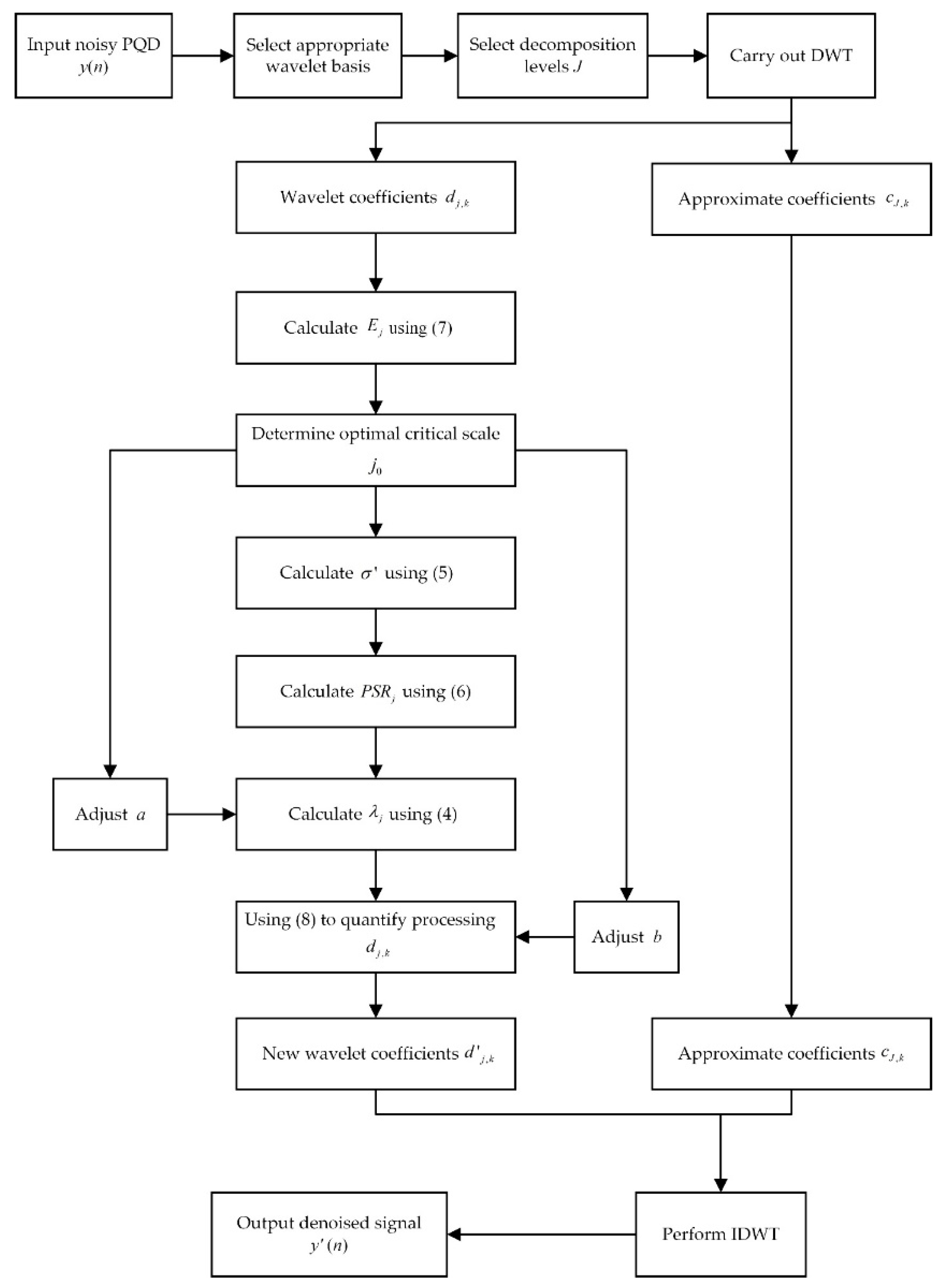
• Signal decomposition. Set sampling frequency $f_s$ and $N$, select an appropriate wavelet basis, ascertain the wavelet decomposition levels $J$, and execute $J$-level wavelet decomposition on the noisy PQD signal to yield approximate coefficients $c_{J,k}$ for the $J$-th level and wavelet coefficients $d_{j,k}$ for each decomposition level $j$ ($j=1,\cdot \cdot \cdot ,J$), where $k$ denotes the $k$-th coefficient. The wavelet coefficients enable signal and noise separation.
• Threshold quantization. The white noise’s standard deviation, $\sigma$, is estimated to be ${\sigma }^{\prime }$, which determines the threshold values. Then, using a threshold function, process the wavelet coefficients $d_{j,k}$ of each level to obtain the estimated wavelet coefficients $d_{j,k}^{\prime }$.
• Signal reconstruction. The inverse discrete wavelet transform (IDWT) is used to obtain the denoised signal $y^{\prime }(n)$ from the new wavelet coefficients $d_{j,k}^{\prime }$ and the unprocessed approximate coefficients $c_{J,k}$.

The function of the hard threshold is defined as follows:

$$d_{j,k}^{\prime }=\{\begin{array}{l}{d}_{j,k}, \left|d_{j,k}\right|\ge \lambda \hfill \\ 0,\left|d_{j,k}\right|<\lambda \hfill \end{array}$$

(2)

The function of the soft threshold is defined as follows:

$$d_{j,k}^{\prime }=\{\begin{array}{l}\mathrm{sgn}(d_{j,k})(\left|d_{j,k}\right|-\lambda ), \left|d_{j,k}\right|\ge \lambda \hfill \\ 0,\left|d_{j,k}\right|<\lambda \hfill \end{array}$$

(3)

where $\mathrm{sgn}$ is the symbolic function; when $d_{j,k}>0$, $\mathrm{sgn}(d_{j,k})=1$; when $d_{j,k}=0$, $\mathrm{sgn}(d_{j,k})=0$; when $d_{j,k}<0$, $\mathrm{sgn}(d_{j,k})=-1$; $\lambda$ is the estimated universal threshold [20].

According to the explanation above, the purpose of wavelet threshold denoising is to convert the noisy PQD signal to the wavelet domain and then process the wavelet coefficients of each level by selecting a suitable threshold and threshold function to obtain new wavelet coefficients. The estimation of the threshold and the establishment of the threshold function are critical processes in wavelet threshold denoising [23]. In wavelet coefficients, threshold denotes the boundary between noise and meaningful signal. The threshold value has a direct effect on the denoising effect. The threshold function is the wavelet shrinking function that specifies how the wavelet coefficients are treated when the threshold is applied.

3. Improved Adaptive Wavelet Threshold Algorithm Based on Energy Optimization

3.1. Adaptive Threshold Correction Based on Energy Optimization

The wavelet coefficients of usable information and noise processed using the discrete wavelet transform (DWT) exhibit a range of features, depending on the wavelet decomposition level. The energy of a valuable signal is concentrated in a few large magnitude wavelet coefficients, whereas the energy of noise is dispersed across the entire wavelet domain via a large number of small magnitude wavelet coefficients [24]. The modulus of the noise’s wavelet coefficients continues to drop as the number of decomposition levels increases [32]. As a result, typical wavelet threshold denoising approaches process each layer of wavelet coefficients using a constant threshold, which introduces substantial deviations into the denoising impact. When wavelet coefficients with a smaller decomposition scale are processed with a fixed threshold, insufficient noise is removed and the denoising effect is poor, whereas when wavelet coefficients with a larger decomposition scale are processed with a fixed threshold, useful information filtering occurs. In light of this characteristic, the decomposition level dependent threshold, which uses $\ln (j+1)$ to correct the universal threshold, is proposed in [2]. The threshold is gradually reduced with the increasing of $j$. The modulus of wavelet coefficients can be used to describe the amount of energy carried by them. When mutation signals are decomposed on a lower scale, their energy content increases dramatically. Thus, the hierarchical estimation criteria discussed previously, which evaluate only the noise distribution, are inapplicable to the mutation signal. As a result, Wang et al. [1] proposed that the stratification threshold be corrected using the PSR. The correction threshold, on the other hand, is relatively fixed. As a result, this article offers an adjustable adaptive wavelet threshold that is not only compatible with the noise distribution at each decomposition size but also with the distribution of meaningful information contained in various forms of disturbance signals at each decomposition scale. The proposed modified threshold is defined as follows:

$${\lambda }_j=\frac{{\sigma }^{\prime }\sqrt{2\ln N}}{\ln (1+(1+a)j)L_j^{PS{R}_j}}(-1\le a\le 1)$$

(4)

$${\sigma }^{\prime }=\frac{median(\left|d_{1,k}\right|)}{0.6745}$$

(5)

where $a$ is the correction factor; $L_j$ is the length of wavelet coefficients with decomposition level of $j$; $d_{1,k}$ is the wavelet coefficient with decomposition level of 1; $PS{R}_j$ is the PSR of wavelet coefficients with decomposition level of $j$, which is defined as follows:

$$PS{R}_j=\frac{\max (\left|d_{j,k}\right|)}{{\displaystyle \sum _{k=1}^{L_j}\left|d_{j,k}\right|}}$$

(6)

When $PS{R}_j$ is large, it indicates that there are a few coefficients with large values in this decomposition level, indicating that this level contains more useful signals. When $PS{R}_j$ is small, it indicates that there are a large number of coefficients with small values, indicating that this level contains more noise [1,24,32].

The adjustment of $a$ improves the precision of the threshold estimate. In order to adjust $a$ adaptively, the idea of optimal critical scale $j_0$ is introduced. After WT decomposes the noisy PQD signal, the noise dominates in the small decomposition level ($j\le j_0$), and the wavelet coefficients of these scales decrease with the increase of $j$, implying that the energy of wavelet coefficients decreases as well with the increase of $j$. In the larger decomposition level ($j>j_0$), the useful signal dominates, and the wavelet coefficient energy is large [33]. The critical scale can be estimated using the wavelet coefficient energy characteristics of the noise and signal following WT. The first extreme point in the wavelet coefficient energy curve appears as $j$ is increased, and the decomposition level corresponding to the extreme point is selected as the optimal critical scale $j_0$. The energy calculation formula of each level is as follows:

$$E_j={\displaystyle \sum _{k=1}^{L_j}{d}_{j,k}^2}$$

(7)

When $j\le j_0$, $a$ takes a smaller value to make ${\lambda }_j$ slightly larger, which is conducive to noise filtering. When $j>j_0$, $a$ takes a larger value to make ${\lambda }_j$ slightly smaller, which is conducive to retaining useful information. According to the experimental statistics, the value of $a$ in this paper is as follows: When $j\le j_0$, $a=-0.25$; when $j>j_0$, $a=0.01$.

According to Equation (4), with the increase of $j$, $\ln (1+(1+a)j)$ gradually increases and ${\lambda }_j$ decreases, which conforms to the general rule that the noise decreases with the increase of decomposition levels. When $j\le j_0$, the value of $a$ can slightly increase ${\lambda }_j$, which is more conducive to noise filtering. When $j>j_0$, the value of $a$ can slightly reduce ${\lambda }_j$, which is conducive to retaining useful information. With the increase of $PS{R}_j$, $L_j^{PS{R}_j}$ gradually increases and ${\lambda }_j$ gradually decreases, which is more conducive to the retention of mutation information and can adapt to the distribution of useful information of different types of disturbance signals in each level. In comparison to [1], the adaptive correction threshold presented in this study is more conducive to denoising harmonics and intricate disturbances with harmonics.

3.2. Improvement of Soft and Hard Threshold Functions

The hard threshold function retains wavelet coefficients with a modulus greater than the threshold and discards those with a modulus less than the threshold, which preserves the signal’s characteristics well but introduces a discontinuity at the set threshold, resulting in serious oscillations during signal reconstruction. While the soft threshold function has a high degree of overall continuity and denoising effect, there is a constant deviation in the wavelet coefficients after threshold quantization, which reduces the wavelet coefficients with a large modulus and is more likely to result in the loss of mutation point energy. As a result, both the soft and hard threshold functions must be enhanced in order to reduce signal reconstruction error. The enhanced threshold function should comply with the following requirements:

• The objective function is consecutive and does not deviate;
• Differentiability of the objective function is essential;
• The objective function’s soft and hard features should be modifiable. When the modulus of the wavelet coefficient exceeds the threshold value, the threshold function is monotonous.

Based on the criteria outlined above, a new improved threshold function is introduced:

$$d_{j,k}^{\prime }=\{\begin{array}{ll}\mathrm{sgn}(d_{j,k})(\left|d_{j,k}\right|-(1-e^{\frac{-b}{\left|d_{j,k}\right|-{\lambda }_j}}){\lambda }_j), \hfill & \hfill \left|d_{j,k}\right|\ge {\lambda }_j \\ 0,\hfill & \hfill \left|d_{j,k}\right|<{\lambda }_j\end{array}$$

(8)

where $b$ is a variable parameter, and different values of $b$ will affect the trend of the improved threshold function; ${\lambda }_j$ is calculated using Equation (4).

The characteristics of the improved wavelet threshold function are as follows:

• When $d_{j,k}={\lambda }_j$, $d_{j,k}^{\prime }=0$; when $d_{j,k}\to {\lambda }_j^{-}$, $d_{j,k}^{\prime }\to 0$; when $d_{j,k}=-{\lambda }_j^{+}$, $d_{j,k}^{\prime }\to 0$. So, the improved wavelet threshold function is continuous at the threshold ${\lambda }_j$. When $d_{j,k}\to \infty$, $e^{-b/(\left|d_{j,k}\right|-{\lambda }_j)}\to 1$ and $d_{j,k}^{\prime }\to d_{j,k}$, the improved threshold function has no deviation, so that the reconstructed signal is closer to the actual value.
• The improved threshold function is a function that has been merged with an exponential function by four fundamental admixture processes, resulting in a function with a high degree of derivability.
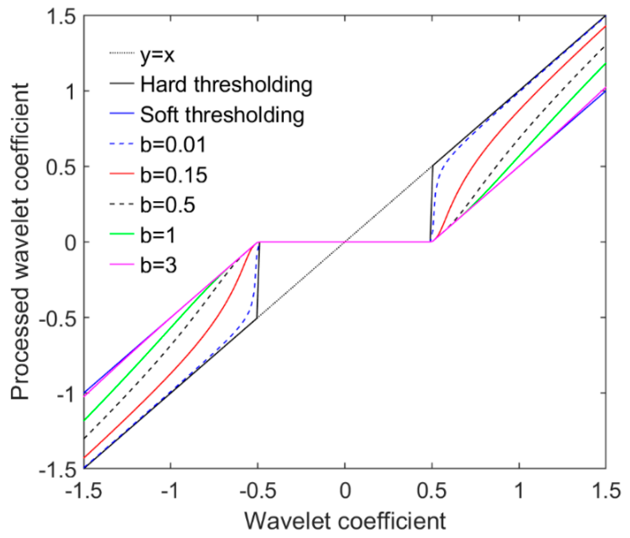
• When $b\to 0$, the improved threshold function is equivalent to the hard threshold function. When $b\to +\infty$, the improved threshold function is equivalent to the soft threshold function. When $b\in (0,+\infty )$, the improved threshold function can switch between soft and hard threshold functions, increasing its flexibility. Simultaneously, it exhibits characteristics of both hard and soft threshold functions. Different threshold functions can be generated by adjusting $b$, as illustrated in Figure 1. Here, the parameter threshold function of each take $\lambda ={\lambda }_j=0.5$, $\left|d_{j,k}\right|\le 1.5$. As illustrated in Figure 1, by gradually increasing $b$, the improved threshold function approaches the soft threshold function. When $b=3$, the improved threshold function approaches the soft threshold function extremely closely. As a result, the value range of $b$ is 0 to 3. However, in order to better fit the denoising of PQD in practical engineering, the value range of $b$ is 0 to 1. Simultaneously, when $b$ is constant, as illustrated in Figure 1, the threshold function is monotonic.

Prior to thresholding the wavelet coefficients, the parameter $b$ must be adaptively adjusted to obtain the corresponding optimal threshold function for the various scale of decomposition. According to the concept of optimal critical scale, when $j\le j_0$, noise has a significant role. The parameter $b$ should be adjusted to move the features of the enhanced wavelet threshold function closer to those of the soft threshold function, which has a greater denoising effect but is not identical to the soft function, in order to prevent exacerbating the energy loss of mutation information taking precedence. When $j>j_0$, the useful signal plays a leading role. The parameter $b$ should be tuned to bring the attributes of the enhanced wavelet threshold function as close to the hard threshold function as possible while minimizing energy loss, but not quite equal to the hard function, in order to minimize the noise residue impairing the denoising impact. In comparison to existing improved threshold function approaches, the value of the suggested improved threshold function’s added adjustment parameter is more transparent and conducive to signal denoising.

The proposed method’s implementation sequence is depicted in Figure 2. The specific implementation steps are as follows:

• Set $f_s$ and $N$ according to the characteristics of noisy PQD signal $y(n)$, select appropriate wavelet basis and wavelet decomposition levels $J$, then carry out DWT to obtain approximate coefficients $c_{J,k}$ and wavelet coefficients $d_{j,k}$.
• The optimal critical scale $j_0$ is determined by computing the energy $E_j$ at each decomposition level using Equation (7).
• The standard deviation $\sigma$ of white noise is estimated using Equation (5) to obtain ${\sigma }^{\prime }$.
• Calculate the $PS{R}_j$ using Equation (6).
• Adjust the parameter $a$ adaptively in accordance with $j_0$, and substitute it into Equation (4) to determine the threshold of each level.
• The parameter $b$ is adaptively adjusted in relation to $j_0$, and the new wavelet coefficients $d_{j,k}^{\prime }$ are obtained by substituting Equation (8) for the wavelet coefficients $d_{j,k}$ processing.
• The IDWT is performed by using $d_{j,k}$ and the unprocessed approximation coefficient $c_{J,k}$ to obtain the denoised signal $y^{\prime }(n)$.

4. Results and Discussion

The experiment was carried out on a computer powered by an Intel Core i5-6200U processor and equipped with 8.0 GB of random access memory (RAM). Seven typical transient disturbances were simulated using MATLAB 2018b based on the mathematical models reported in [34], and Gaussian white noise with a SNR of 50 dB to 10 dB was added. There were five types of single disturbances: voltage interruption, sag, swell, impulsive transient, and oscillatory transient. There were also two composite disturbance signals: harmonics with voltage sag and harmonics with swell. The following experimental parameters were defined: $f_s=\mathrm{12,800} \mathrm{Hz}$, $N=2048$. When denoising signals with wavelet analysis, selecting the optimal wavelet basis can enhance the denoising effect. The Daubechies wavelet is orthogonal and has a high degree of support. It exhibits a high degree of sensitivity for detecting signal mutation points. It is a wavelet function in its ideal state, according to [35], and the db4 wavelet is the most suitable for identifying transient power quality disturbances. Therefore, the db4 wavelet was used as the basis for the wavelet decomposition, and the signal was decomposed into five layers. To demonstrate the proposed denoising algorithm’s denoising effect, the traditional soft and hard thresholding denoising algorithms, three improved wavelet threshold denoising algorithms proposed in [1,2,27], named as improved method 1, improved method 2 and improved method 3 respectively and the proposed wavelet threshold adaptive denoising algorithm were used to denoise the above seven power quality signals at various noise intensities. The SNR and MSE of the reconstructed signal were used to quantify the denoising effect of each method. The higher the SNR and the lower the MSE, the more effective the denoising effect. SNR and MSE are defined as follows [31]:

$$\mathrm{SNR}=10\lg \frac{{\displaystyle \sum _{n=1}^{N}x{(n)}^2}}{{\displaystyle \sum _{n=1}^N{\left|x(n)-y^{\prime }(n)\right|}^2}}$$

(9)

$$\mathrm{MSE}=\frac{1}{N}{\displaystyle \sum _{n=1}^N{\left|x(n)-y^{\prime }(n)\right|}^2}$$

(10)

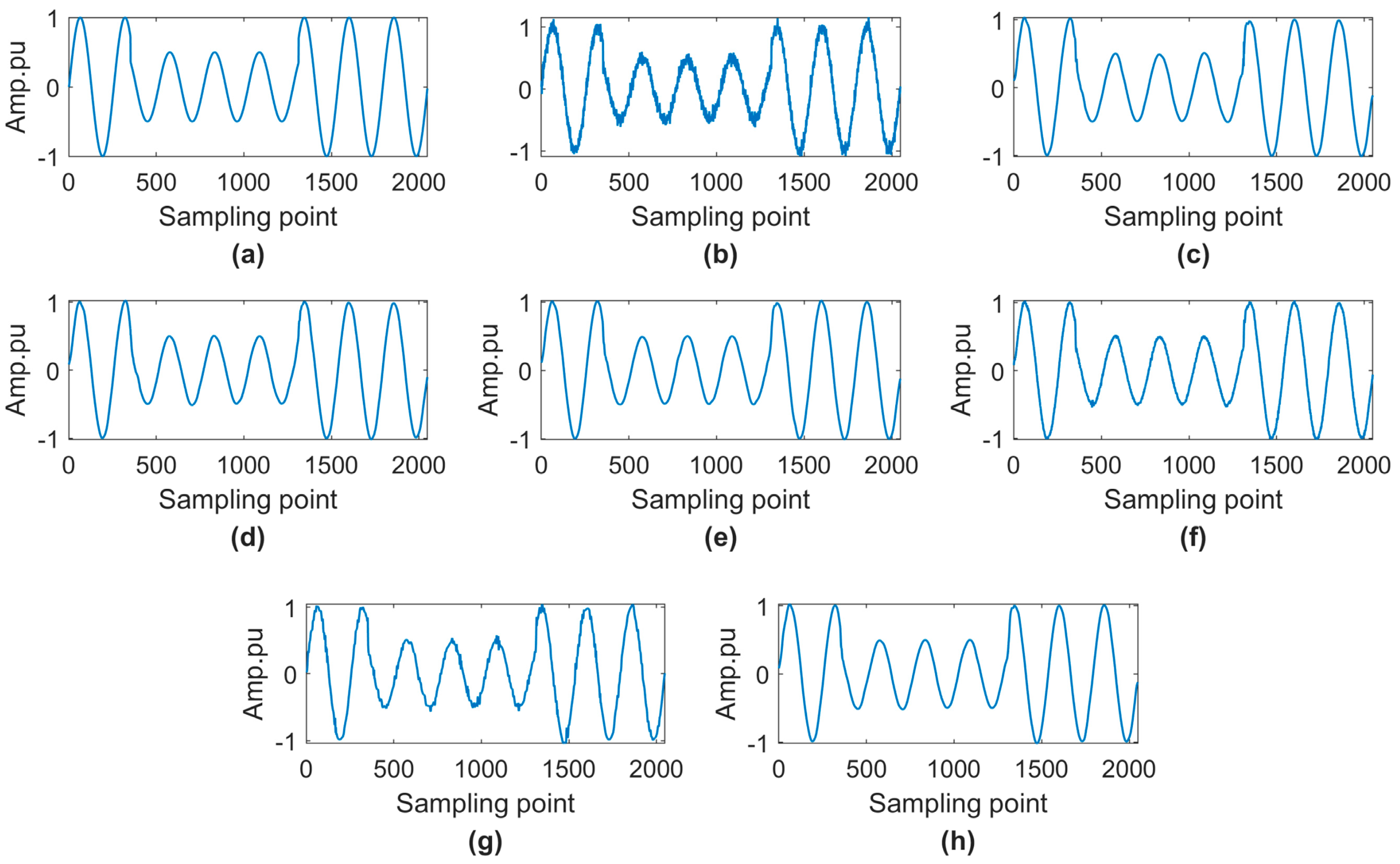
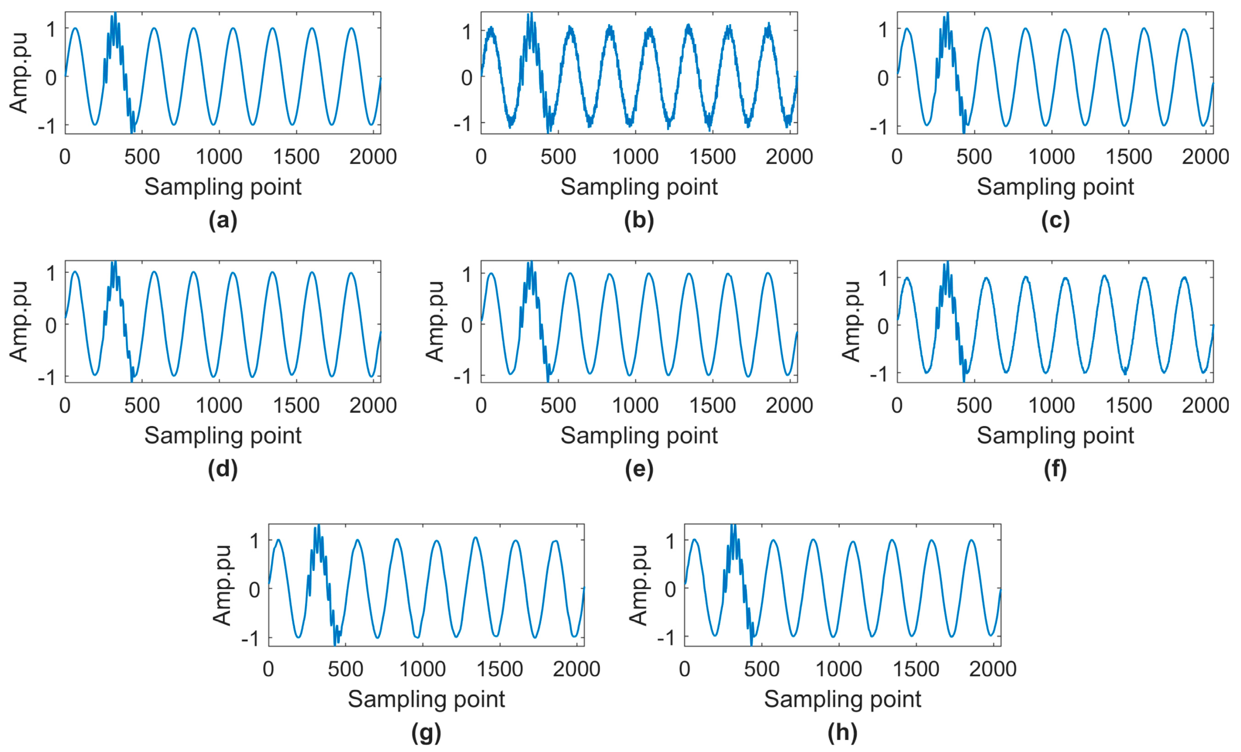
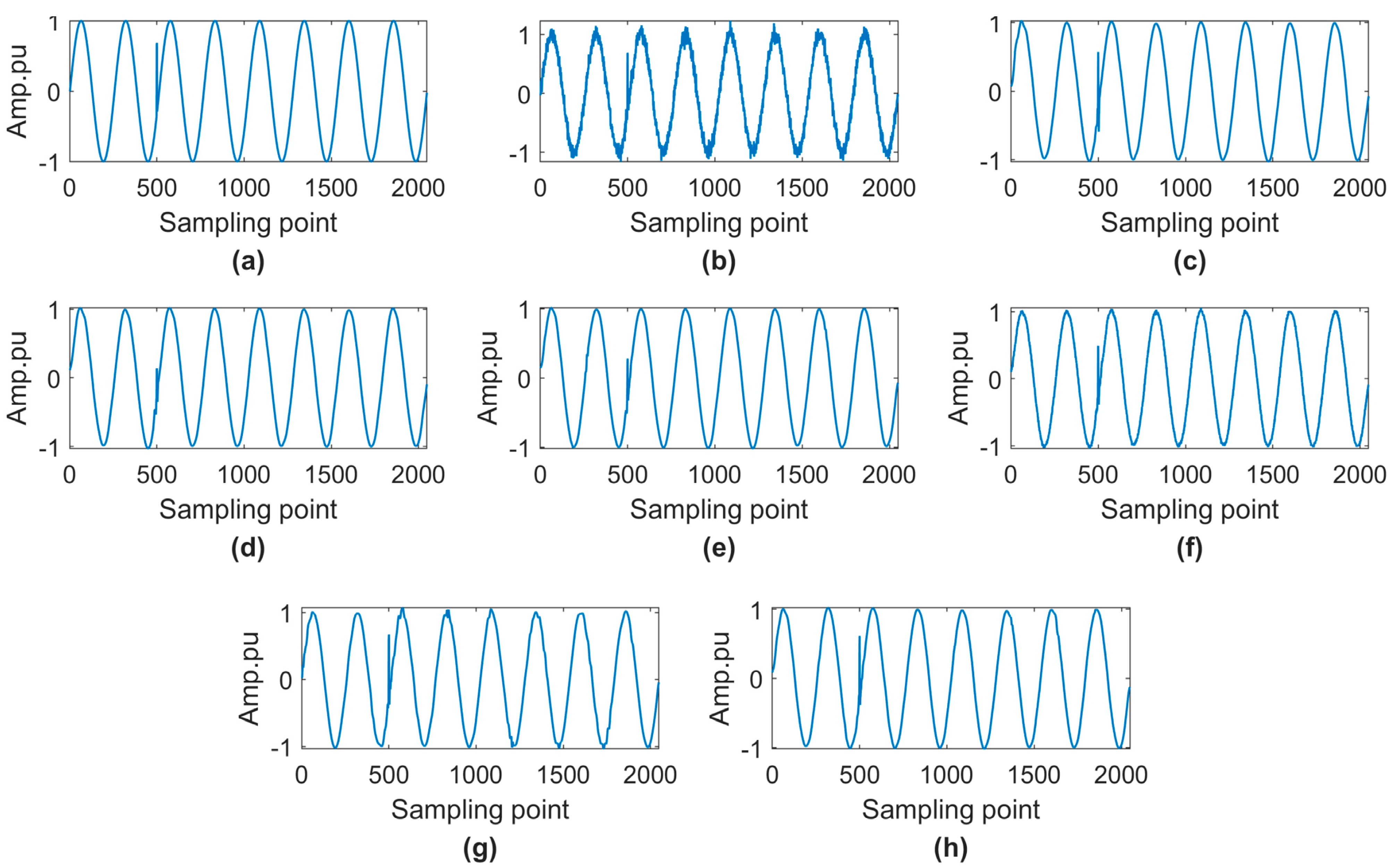
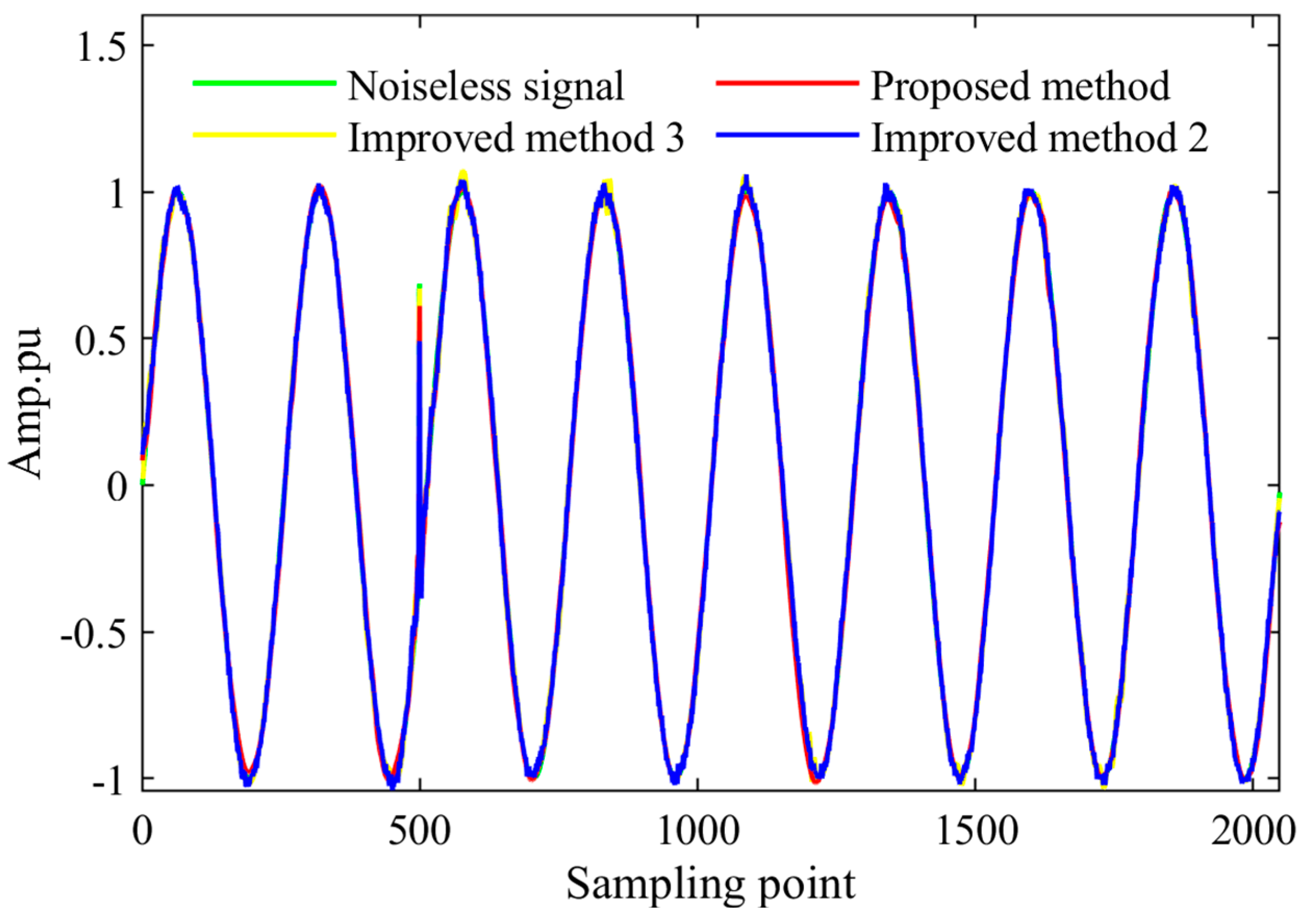
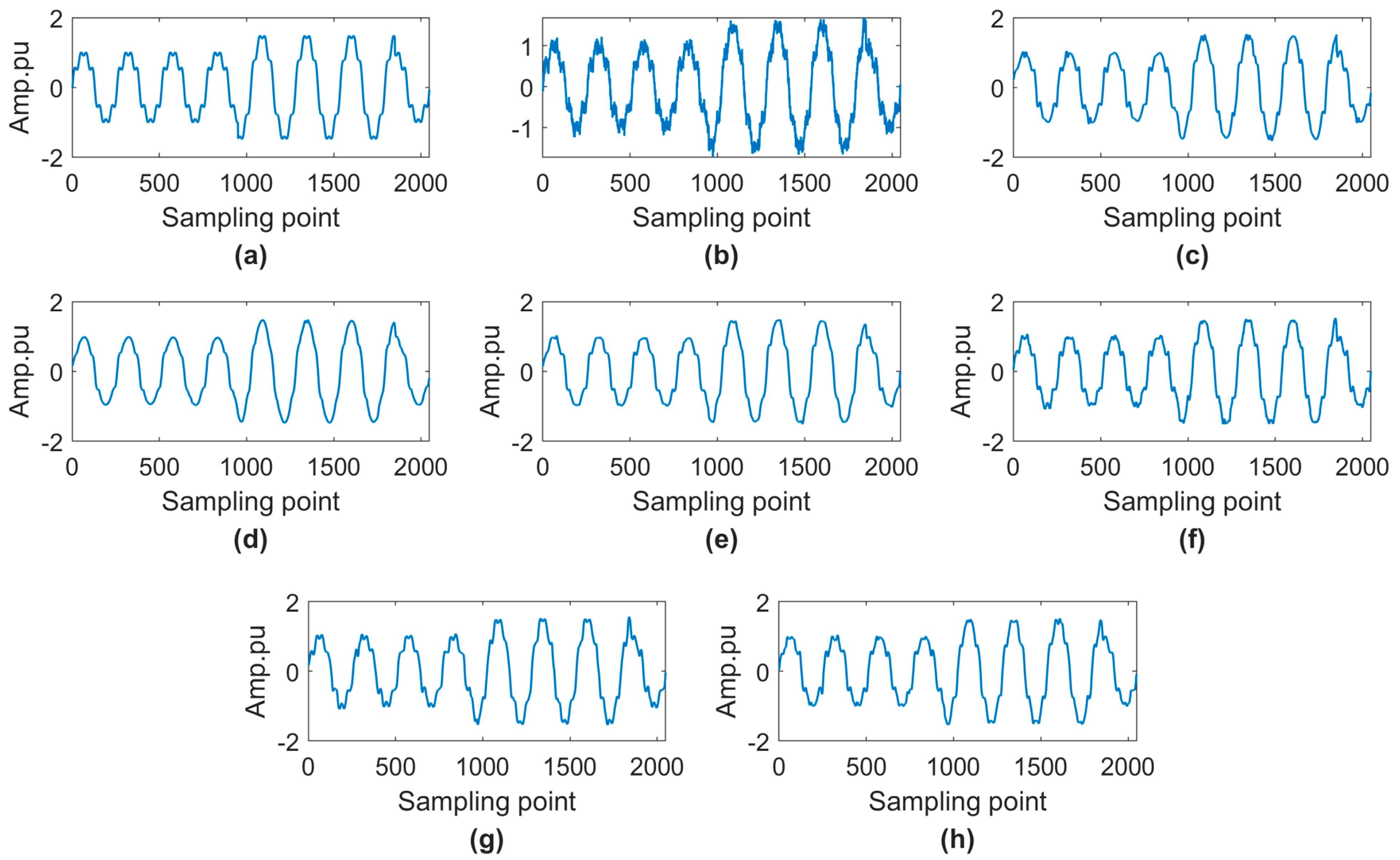
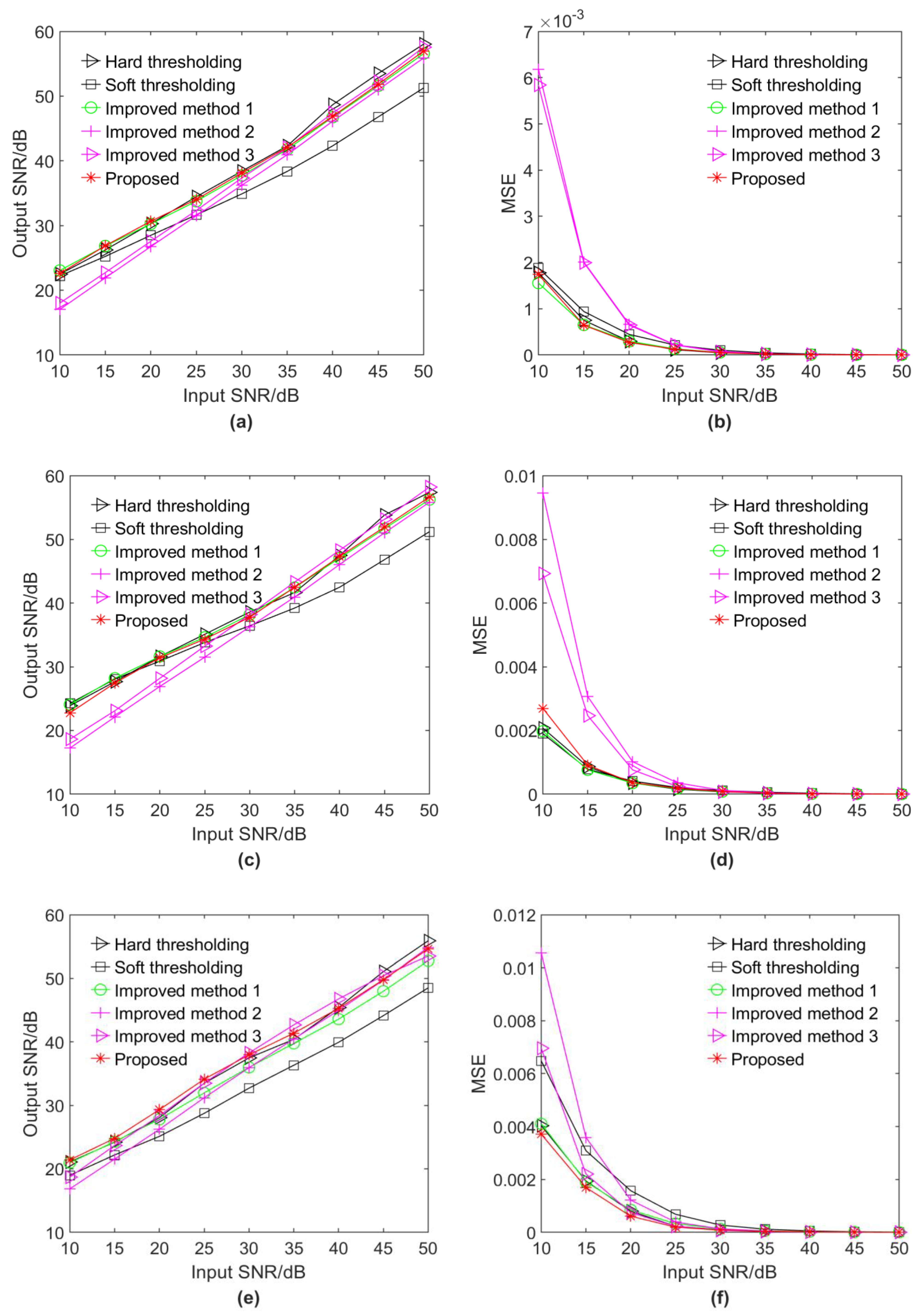
4.1. Denoising Effects on Transient PQDs

To demonstrate the effectiveness of the proposed denoising algorithm, voltage sag, oscillation transient, impulsive transient, and harmonics with swell were used as examples to denoise. For each disturbance, Gaussian white noise with an SNR of 20 dB was added. Each noisy disturbance was denoised using the six methods described above, and the denoised signals are shown in Figure 3, Figure 4, Figure 5 and Figure 6 to illustrate the experimental results more clearly. The denoised signals’ SNR and MSE values are listed in

Table 1. Denoising effect of various methods on PQDs with a 20 dB SNR.

Methods	Output SNR (dB)/MSE
	Voltage Sag	Oscillation Transient	Impulsive Transient	Harmonics with Swell
Hard thresholding	30.1952/ 3.1710 × 10−4	28.1568/ 7.7107 × 10−4	30.6711/ 4.2870 × 10−4	23.3452/ 3.6720 × 10−3
Soft thresholding	29.4914/ 3.7289 × 10−4	25.4832/ 1.4271 × 10−3	29.0017/ 6.2964 × 10−4	21.2288/ 5.9778 × 10−3
Ref. [1]	30.2688/ 3.1177 × 10−4	28.0887/ 7.8327 × 10−4	30.4294/ 4.5324 × 10−4	23.9591/ 3.1879 × 10−3
Ref. [2]	29.9051/ 3.3900 × 10−4	28.6087/ 6.9489 × 10−4	30.2666/ 4.7055 × 10−4	25.5215/ 2.2246 × 10−3
Ref. [27]	25.4180/ 9.5261 × 10−4	27.1797/ 9.6562 × 10−4	29.6927/ 5.3703 × 10−4	24.9874/ 2.500 × 10−3
Proposed method	30.4759/ 2.9725 × 10−4	29.1354/ 6.1552 × 10−4	31.1783/ 3.8145 × 10−4	26.0748/ 1.9585 × 10−3

.

The noiseless voltage sag and the voltage sag with an SNR of 20 dB, sag amplitude of 0.5 pu, and disturbance starting and ending points of 352 and 1312, respectively, are shown in Figure 3a,b. The signals in Figure 3c–h were produced after denoising the noisy signal in Figure 3b using various denoising techniques. By examining the waveform in Figure 3g, it is obvious that even after denoising using the method suggested in [27], a significant amount of noise remained in the data. According to the approach provided in [2], there were clear abrupt changes in the waveform obtained after denoising the noisy voltage sag during the disturbance, as illustrated in Figure 3f, which would impact the start and finish points of the disturbance. By examining the waveforms in Figure 3c–h and comparing them to the SNR and MSE values in Table 1, it is clear that, except for the approach proposed in [27], the proposed method’s denoising effect is comparable to that of the other four methods, but the suggested method is superior. Additionally, it is worth noting that, when compared to the approach proposed in [27], the SNR of the denoised signal obtained using the suggested method was enhanced by 5.0579 dB and the MSE was decreased by 68.8%.

The noiseless oscillation transient and the oscillation transients with an SNR of 20 dB in Figure 4a,b have an amplitude of 0.4 pu, an attenuation coefficient of 0.04 s, a frequency of 550 Hz, and disturbance start and end points of 250 and 450, respectively. The signals in Figure 4c–h were produced after denoising the noisy signal in Figure 4b using various denoising techniques. In terms of signal disturbance feature retention, it is clear from Figure 4d that the disturbance mutation position of the signal obtained after soft threshold denoising is smoother, indicating that the soft threshold denoising method is ineffective at signal disturbance feature retention, which is detrimental to subsequent disturbance detection. As illustrated in Figure 4f, the waveform generated after denoising the noisy oscillation transient using the method proposed in [2] produces sudden changes in the non-disturbance segment of the original signal, which leads to misjudgment of disturbance location. As shown in Table 1, the denoising effect of soft threshold is the worst for the noisy oscillation transient signal, whereas the suggested technique has the best denoising effect. Additionally, as compared to the soft thresholding denoising effect, the suggested method enhances the SNR by 3.6522 dB and reduces the MSE by 56.9%.

The noiseless impulsive transient and the impulsive transient with an SNR of 20 dB, impulsive amplitude of 1 pu, and disturbance starting and ending points of 498 and 500, respectively, are depicted in Figure 5a,b. By comparing the waveforms in Figure 5a–h, it is easy to see how well each denoising approach retains the disturbance characteristics of the original signal. As illustrated in Figure 5c, hard thresholding advances the mutation point of the disturbance, which is detrimental to disturbance identification. Observing the waveforms in Figure 5d,e demonstrates the weakness of the approach presented in [1] in keeping the disturbance characteristics of the original signal. To facilitate comparison of the denoising impacts of several approaches, the waveforms in Figure 5a,f–h are combined into a single plot, as shown in Figure 7. As illustrated in Figure 7, the method proposed in [27] retains the disturbance characteristics more effectively than the current method. However, as shown in Table 1, the suggested method improves the SNR by 1.4856 dB and reduces the MSE by 29.9 percent when applied to noisy impulsive transient signals, as compared to the method proposed in [27]. In comparison to the soft thresholding method with the least effective denoising for impulsive transients, the denoising method described in this work improves the SNR by 2.1766 dB and reduces the MSE by 39.4%.

The noiseless voltage swell with third, fifth, and seventh harmonic components is illustrated in Figure 7a, where the swell amplitude is 0.5 pu, the disturbance’s starting and ending points are 950 and 1850, and the amplitudes of the third, fifth, and seventh harmonics are 0.05 pu, 0.1 pu, and 0.15 pu, respectively. Figure 7b illustrates the harmonics with swell at a 20 dB SNR. The signals in Figure 7c–h were produced after denoising the noisy signal in Figure 7b using various denoising techniques. As illustrated in Figure 7d,e, soft thresholding and the approach presented in [1] are ineffective for denoising disturbances with harmonics. As shown in Table 1, the soft threshold denoising effect is the worst for denoising noisy harmonics with swell. The proposed method has the best denoising effect, followed by the method provided in [2]. In comparison to the soft threshold, the strategy suggested in this article enhances SNR by 4.8460 dB and decreases MSE by 67.2%. In comparison to the strategy described in [2], the method provided in this paper reduces the MSE by 12.0%.

To summarize, the soft threshold denoising algorithm has a poor overall denoising effect, is prone to smoothing out the original signal’s disturbance characteristics, and is incompatible with denoising disturbances with harmonics. While hard thresholding has a considerable denoising effect, the denoised signal will exhibit apparent oscillation at the mutation point, which is inconvenient for detecting and localizing disturbances. While the method presented in [1] has a good overall denoising impact and produces a smoother denoised signal, it also smooths out essential disturbance characteristic information, which is incompatible with denoising complicated disturbances with harmonics. The method presented in [2] provides an excellent overall denoising effect and is also suitable for denoising disturbances with harmonics. While the retention of disturbance characteristic signals is superior to that of soft thresholding and the method proposed in [1], the waveform obtained after denoising fluctuates in both disturbance and non-disturbance segment of original signal, which is detrimental to subsequent disturbance detection and location. Although the approach presented in [27] offers more advantages in terms of keeping disturbance-specific information, its denoising effect is minimal. After denoising, the signal contains additional noise. In comparison, the denoising method suggested in this study not only performs well but also retains more of the original signal’s disruption characteristics. Second, the denoised signal’s non-disturbance period is smoother, avoiding oscillations around the disturbance mutation point or forward movement of the disturbance mutation point. It is also applicable to harmonic disturbances.

To demonstrate the algorithm’s denoising effect further, the five methods described above are used to denoise voltage interruption, impulsive transient, oscillatory transient, and harmonics with sag under various noise intensities. The output SNRs and MESs of denoising the PQDs using different algorithms are shown in Figure 8. Due to noise’s high randomness, different methods were used to denoise noisy disturbances, and the output SNR and MSE values are the averages of 50 runs under the same experimental premise.

As indicated in Figure 8, soft thresholding and the approach presented in [27] have a minor effect on total denoising, particularly for disturbances involving harmonics. As illustrated in Figure 8a–d, when the input SNR is low, the denoising effect of the method in [2] is poor, while the denoising effect of the new method, hard thresholding, and the method in [1] are similar, with the new method slightly better. When the input SNR is high, the effect of hard threshold denoising is optimal. As illustrated in Figure 8e,f, the proposed method’s denoising effect is superior to that of the method in [1]. When the input SNR is less than 35 dB, this method outperforms the other four methods in terms of PQD denoising and practical application. The diagrams in Figure 8g,h illustrate the denoising effect of a disturbance with harmonic components. As can be seen, the proposed method is superior to that in [1]. When the input SNR is between 10 dB and 20 dB, the proposed method has a better denoising effect. When the noise intensity is reduced, the new method’s denoising effect approaches that of the method proposed in [2] and hard thresholding.

As illustrated in Figure 3, Figure 4, Figure 5, Figure 6, Figure 7 and Figure 8, the proposed method has a favorable overall denoising effect, particularly in noisy environments. Second, it can adapt to different types of power quality disturbances and maintain a good denoising effect, particularly for disturbances with harmonic components. Simultaneously, the proposed method can better maintain information about mutation points, which aids in the detection of disturbances. Denoising signals is a critical component of PQ monitoring and analysis. As a result, the analysis method must be capable of real-time performance in order to be used in practice. The total duration of 100 experiments is 35.681920 s, or 0.35681920 s for each experiment. As a result, the denoising algorithm presented in this paper not only performs well but also has a short calculation time.

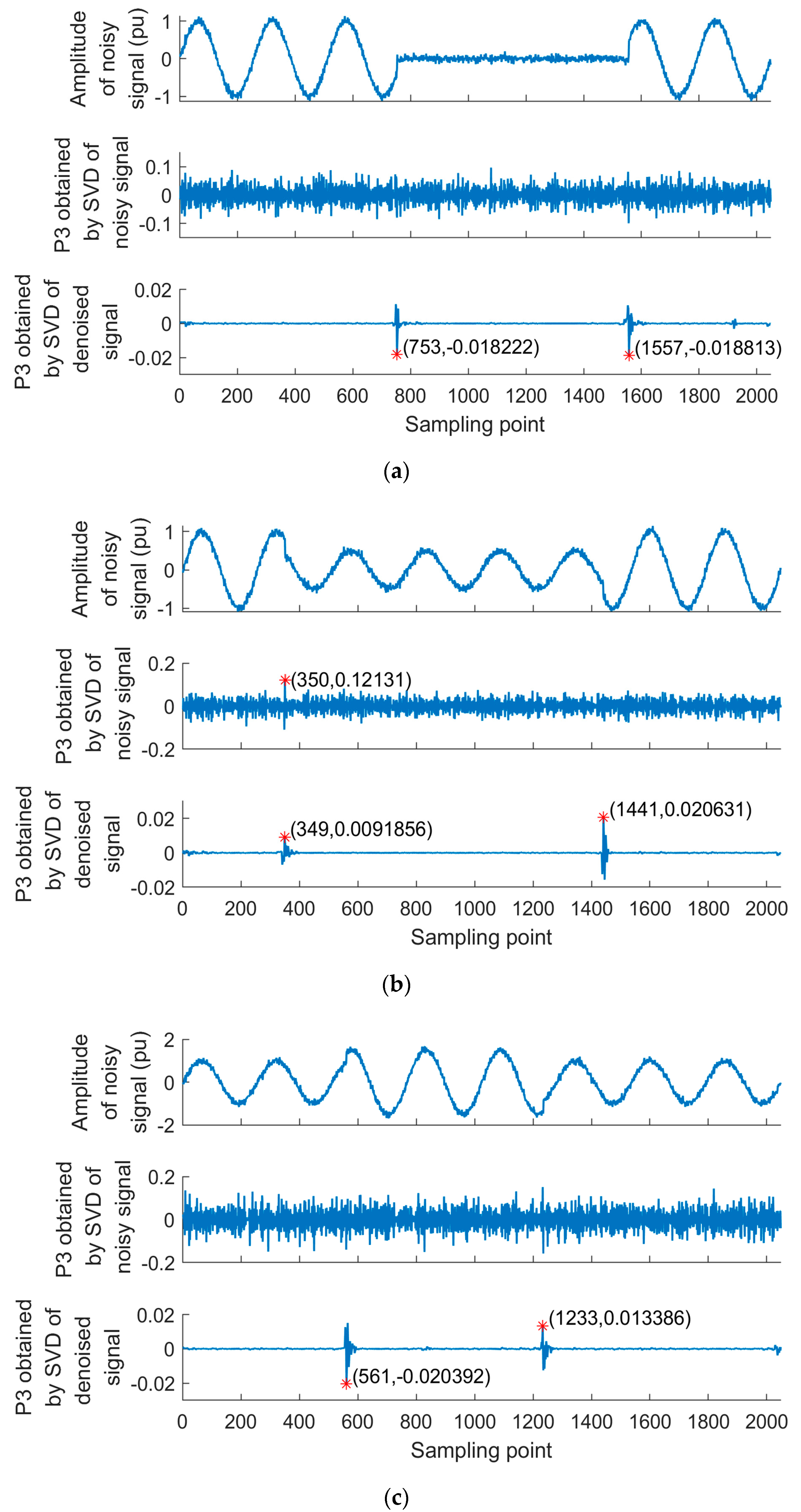
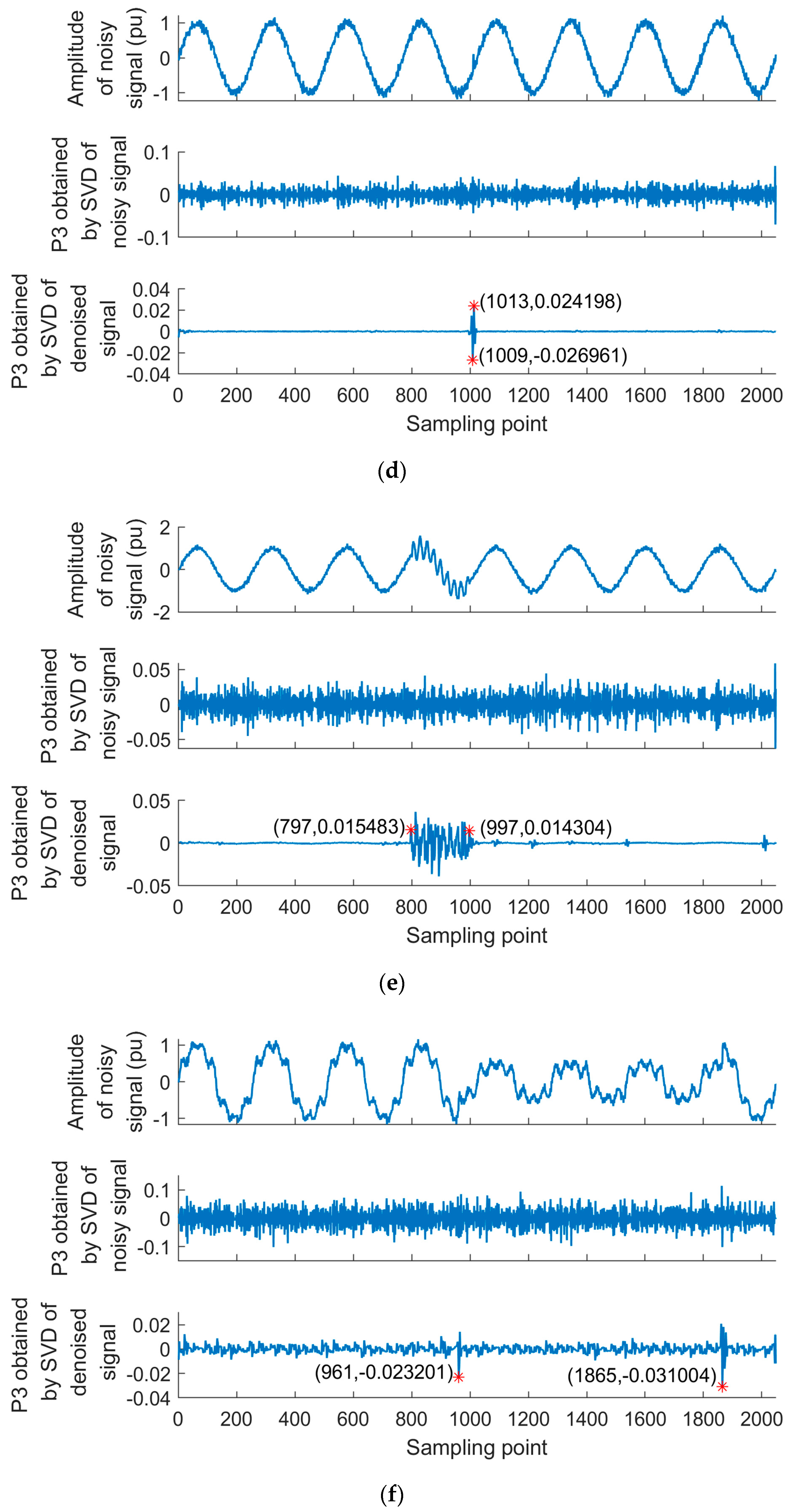
4.2. Location of Denoised Signals Based on SVD

To demonstrate that the proposed method can effectively denoise signals, the proposed method was used to denoise seven disturbances with a SNR of 20 dB, and then SVD was used to locate the denoised signals. The detailed SVD disturbance location procedure is described in detail in [36]. The location of various disturbances is depicted in Figure 9, showing that the disturbance points cannot be accurately identified in the strong noise environment. In Figure 9, P3 represents the third layer component extracted after four decompositions of the signal based on SVD.

The start and end points of the noisy voltage interruption are 753 and 1556, respectively, and the location results are shown in in Figure 9a, implying that the disturbance location error is 0 and 2 points, respectively. As shown in Figure 9b, the location error of the disturbance start point and end point are both equal to one for the noisy voltage sag that begins at point 350 and ends at point 1440. The location error of the disturbance’s start and end points is 1 and 2 points, respectively, for the noisy voltage swell that begins at point 560 and ends at point 1235, as shown in Figure 9c. As shown in Figure 9d, the location error of the disturbance start point and end point are both equal to one for the noisy impulsive transient that begins at point 1010 and ends at point 1012. As shown in Figure 9e, the location error of the disturbance’s start and end points is three and two points, respectively, for the noisy oscillatory transient that begins at point 800 and ends at point 995. For the noisy harmonics with sag that begin at point 960 and end at point 1865, the location error between the disturbance’s start and end points is 1 and 0, as shown in Figure 9f. The location error of the disturbance start point and end point are both one for the noisy harmonics with swell that begin at point 576 and end at point 1472, as shown in Figure 9g.

As shown in Figure 9, the experimental results indicate that when a noisy disturbance occurs, the mutation information is obscured by the noise, and the disturbance cannot be located using SVD. However, after denoising the noisy signal using the proposed method and then performing SVD detection, the disturbance mutation point can be accurately detected, and the disturbance location error is 0–3 disturbance points, indicating that the proposed method has a good denoising effect and can effectively preserve important mutation point information, allowing SVD to accurately detect and locate PQDs even in a noisy environment.

5. Conclusions

To adapt to the effective denoising of various types of transient disturbances while retaining critical disturbance information, this paper proposes an improved adaptive wavelet threshold denoising algorithm based on energy optimization. The main goal of this paper is to propose an improved method that addresses the shortcomings of the traditional soft and hard threshold methods and to make explicit provisions regarding the value of the introduced parameters, such that the introduced parameters’ values can be adjusted adaptively in response to different types of disturbances, resulting in a more effective denoising effect.

The performance of the proposed algorithm is then evaluated by denoising various types of transient disturbances at various noise levels, and the results are compared to those obtained using soft and hard thresholding, as well as the other three wavelet threshold improvement methods proposed in [1,2,27].

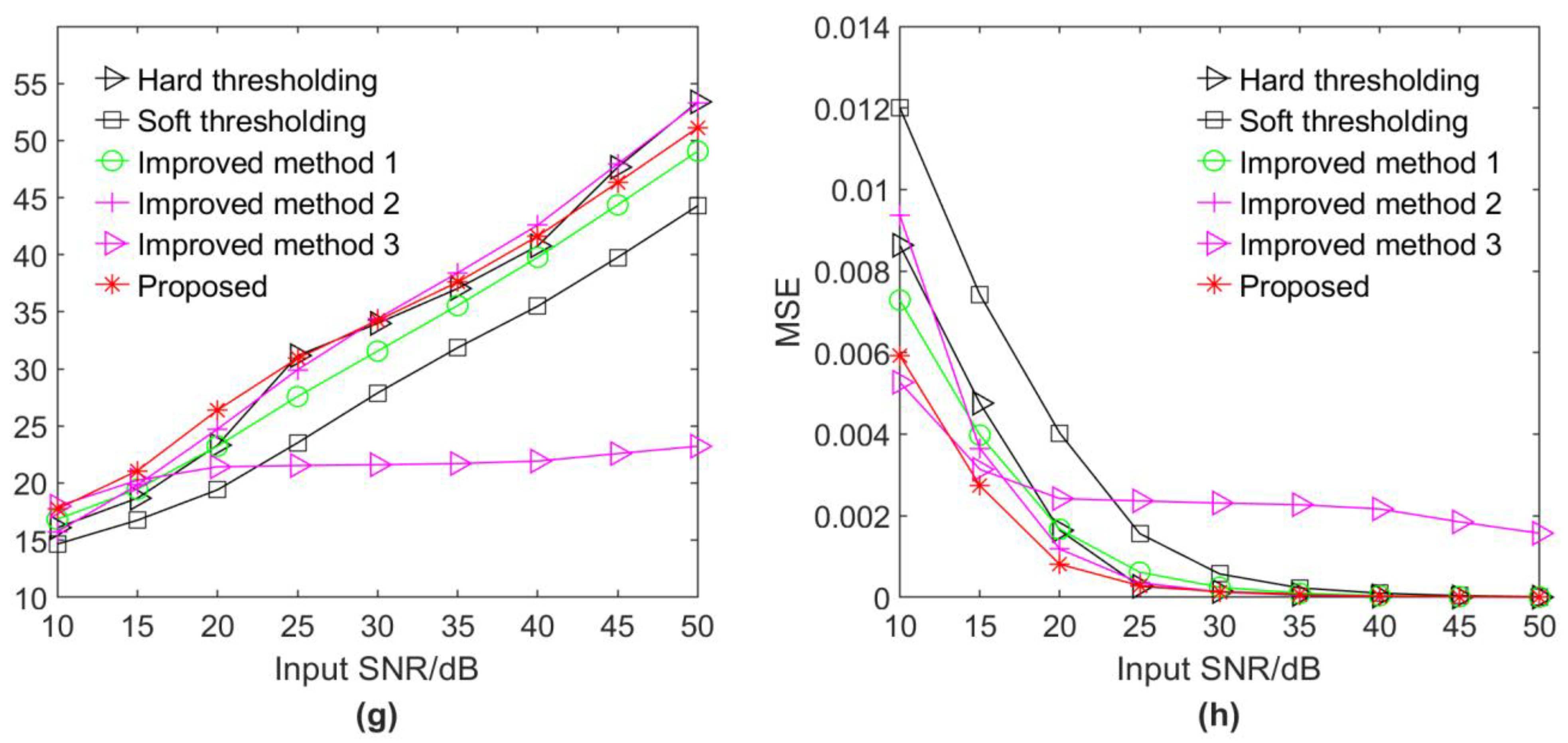
• Denoising findings for four disturbances with an SNR of 20 dB using the proposed technique and five comparison methods indicate that the suggested method has the best overall denoising effect, the maximum SNR can be enhanced by 5.0579 dB, and the corresponding MES is decreased by 68.8 percent. Additionally, the proposed method can keep a greater amount of the original signal’s disturbance characteristic signal during the de-noising process.
• The denoising results of various methods for different types of disturbances denoising in various noise environments further indicate that soft thresholding and the proposed method in [27] have a poor overall denoising effect and are therefore unsuitable for denoising disturbances containing harmonics. Hard thresholding and the improved wavelet threshold denoising method proposed in [2] are more suitable for denoising PQDS in low-noise environments (SNR greater than 30 dB), whereas soft thresholding has a poor overall denoising effect. Because the variable parameter value of the improved threshold function proposed in [1] is unknown, it cannot be used for denoising all types of disturbances. In comparison, the proposed method has a favorable overall denoising effect and is applicable to a wide variety of power quality disturbance signals. It has more advantages, in particular, when the disturbance occurs in a noisy environment with a SNR of 10 dB to 20 dB, which reflects the essence of the need for signal denoising, which is quite different from the characteristics of other methods, which have more advantages in a quiet environment.
• The disturbance location results demonstrate that after denoising with the proposed method, SVD can accurately detect the start and end times of disturbances that are heavily polluted by noise with a small error that does not exceed three disturbance points; the minimum error is 0, demonstrating that this method not only effectively denoises, but also effectively retains the characteristics of disturbance information.

The usefulness of this study is demonstrated by evaluating typical transient PQDs; however, no examination of disturbances containing a variety of abrupt signals, such as voltage sag with oscillatory transient, is included in this paper. Based on the method’s central concept of denoising, future work should investigate whether it can be denoised effectively and retain a greater number of mutation points when multiple transient disturbances coexist and multiple mutation points appear. As a result, a more adaptable new method for multi-objective control is required, capable of effectively denoising complex disturbances in a high-noise environment.

References

1. Wang, W.; Dong, R.; Zeng, W.; Zhang, B.; Zheng, Y. A wavelet de-noising method for power quality based on an improved threshold and threshold function. Trans. China Electrotech. Soc. 2019, 34, 409–418. [Google Scholar]
2. Wang, Y.; Xu, C.; Wang, Y.; Cheng, X. A comprehensive diagnosis method of rolling bearing fault based on CEEMDAN-DFA-improved wavelet threshold function and QPSO-MPE-SVM. Entropy 2021, 23, 1142. [Google Scholar] [CrossRef] [PubMed]
3. Yang, H.; Liao, C. A de-noising scheme for enhancing wavelet-based power quality monitoring system. IEEE Trans. Power Deliv. 2001, 16, 353–360. [Google Scholar] [CrossRef]
4. Yang, Z.; Hua, H.; Cao, J. A novel multiple impact factors based accuracy analysis approach for power quality disturbance detection. CSEE JPES 2020, 1–12. [Google Scholar] [CrossRef]
5. Wang, Y.; Li, Q.; Zhou, F. Transient power quality disturbance denoising and detection based on improved iterative adaptive kernel regression. J. Mod. Power Syst. Clean Energy 2019, 7, 644–657. [Google Scholar] [CrossRef] [Green Version]
6. Laurent, G.; Gilles, P.; Woelffel, W.; Barret-Vivin, V.; Gouillart, E.; Bonhomme, C. Denoising applied to spectroscopies—Part II: Decreasing computation time. Appl. Spectrosc. Rev. 2020, 55, 173–196. [Google Scholar] [CrossRef] [Green Version]
7. Ye, B.; Zhou, K.; Huang, Y.; Liu, L.; Zhang, Q. A white nosie suppression method for partial discharge based on AWM and OSVD. Proc. CSEE 2021, 41, 3978–3987. [Google Scholar]
8. Hu, W.; Su, H.; Luan, Y. Power quality signals’ de-noising method based on singular value decomposition (SVD). Power Syst. Prot. Control 2010, 38, 30–33. [Google Scholar]
9. Shukla, S.; Mishra, S.; Singh, B. Power quality event classification under noisy conditions using EMD-based de-noising techniques. IEEE Trans. Ind. Inform. 2014, 10, 1044–1054. [Google Scholar] [CrossRef]
10. Wang, L.; He, Z.; Zhao, J.; Zhang, H. Wavelet transform and mathematical morphology’s application in power disturbance signal denosing. Power Syst. Prot. Control 2008, 36, 30–35. [Google Scholar]
11. Xi, Y.; Li, Z.; Tang, X.; Zeng, X. Classification of power quality disturbances based on KF-ML-aided S-transform and multilayers feedforward neural networks. IET Gener. Transm. Distrib. 2020, 14, 4010–4020. [Google Scholar] [CrossRef]
12. Chen, W.; Li, J.; Wang, Q.; Han, K. Fault feature extraction and diagnosis of rolling bearings based on wavelet thresholding denoising with CEEMDAN energy entropy and PSO-LSSVM. Measurement 2021, 172, 108901. [Google Scholar] [CrossRef]
13. Shen, Y.; Wai, R. Wavelet-analysis-based singular-value-decomposition algorithm for weak arc fault detection via current amplitude normalization. IEEE Access 2021, 9, 71535–71552. [Google Scholar] [CrossRef]
14. Kuang, W.; Wang, S.; Lai, Y.; Ling, W. Efficient and adaptive signal denoising based on multistage singular spectrum analysis. IEEE Trans. Instrum. Meas. 2021, 70, 1–20. [Google Scholar] [CrossRef]
15. Zhao, X.; Ye, B.; Chen, T. Difference spectrum theory of singular value and its application to the fault diagnosis of headstock of lathe. J. Mech. Eng. 2010, 46, 100–108. [Google Scholar] [CrossRef]
16. Wu, Z.; Huang, N.E. A study of the characteristics of white noise using the empirical mode decomposition method. Proc. R. Society. A Math. Phys. Eng. Sci. 2004, 460, 1597–1611. [Google Scholar] [CrossRef]
17. Torres, M.E.; Colominas, M.A.; Schlotthauer, G.; Flandrin, P. A complete ensemble empirical mode decomposition with adaptive noise. In Proceedings of the IEEE International Conference on Acoustics, Prague, Czech Republic, 22–27 May 2011. [Google Scholar]
18. Dwivedi, U.D.; Singh, S.N. Enhanced detection of power-quality events using intra and interscale dependencies of wavelet Coefficients. IEEE Trans. Power Deliv. 2010, 25, 358–366. [Google Scholar] [CrossRef]
19. Wang, R.; Cai, W.; Wang, Z. A New Method of Denoising Crop Image based on improved SVD in wavelet domain. Secur. Commun. Netw. 2021, 2021, 9995813. [Google Scholar] [CrossRef]
20. Donoho, D.L. De-noising by soft-thresholding. IEEE Trans. Inform. Theory 1995, 41, 613–627. [Google Scholar] [CrossRef] [Green Version]
21. Li, J.; Cheng, C.; Jiang, T.; Grzybowski, S. Wavelet de-noising of partial discharge signals based on genetic adaptive threshold estimation. IEEE Trans. Dielectr. Electr. Insul. 2012, 19, 543–549. [Google Scholar] [CrossRef]
22. Fan, X.; Xie, W.; Jiang, W.; Li, Y.; Huang, X. An improved threshold function method for power quality disturbance signal de-noising based on stationary wavelet transform. Trans. China Electrotech. Soc. 2016, 31, 219–226. [Google Scholar]
23. Lu, J.; Lin, H.; Ye, D.; Zhang, Y. A new wavelet threshold function and denoising application. Math. Probl. Eng. 2016, 2016, 3195492. [Google Scholar]
24. Srivastava, M.; Anderson, C.L.; Freed, J.H. A new wavelet denoising method for selecting decomposition levels and noise thresholds. IEEE Access 2016, 4, 3862–3877. [Google Scholar] [CrossRef] [PubMed]
25. Wang, Y.; Zhang, B.; Ding, F.; Ren, H. Estimating dynamic motion parameters with an improved wavelet thresholding and inter-scale correlation. IEEE Access 2018, 6, 39827–39838. [Google Scholar] [CrossRef]
26. Sun, K.; Zhang, J.; Shi, W.; Gou, J. Extraction of partial discharge pulses from the complex noisy signals of power cables based on CEEMDAN and wavelet packet. Energies 2019, 12, 3242. [Google Scholar] [CrossRef] [Green Version]
27. Gong, J. Wavelet denoising method for power quality disturbances based on adjustable threshold function and energy threshold optimization. J. Electron. Meas. Instrum. 2021, 35, 137–145. [Google Scholar]
28. Deng, G.; Ye, J.; Wang, G.; Zhang, F. Signal denoising method based on bee colony algorithm and new threshold function. Appl. Res. Comput. 2019, 36, 2974 2976, 3007. [Google Scholar]
29. Ma, Y.; Zhu, J.; Huang, J. Wavelet denoising of remote sensing image based on adaptive threshold function. In Proceedings of the 3rd International Conference on Video and Image Processing, Shanghai, China, 20–23 December 2019. [Google Scholar]
30. Ray, P.; Maitra, A.K.; Basuray, A. A new threshold function for de-noising partial discharge signal based on wavelet transform. In Proceedings of the International Conference on Signal Processing, Image Processing and Pattern Recognition, Coimbatore, India, 7–8 February 2013. [Google Scholar]
31. Tang, J.; Zhou, S.; Pan, C. A denoising algorithm for partial discharge measurement based on the combination of wavelet threshold and total variation theory. IEEE Trans. Instrum. Meas. 2020, 69, 3428–3441. [Google Scholar] [CrossRef]
32. Srivastava, M.; Georgieva, E.R.; Freed, J.H. A new wavelet denoising method for experimental time-domain signals: Pulsed dipolar electron spin resonance. J. Phys. Chem. A 2017, 121, 2452–2465. [Google Scholar] [CrossRef] [Green Version]
33. Zhang, Q.; Liu, H.; Lan, Q. Power quality signal denoising based on wavelet hybrid threshold method. Electr. Power Autom. Equip. 2008, 28, 28–30, 35. [Google Scholar]
34. Wang, Y.; Li, Q.; Zhou, F.; Zhou, Y.; Mu, X. A new method with Hilbert Transform and slip-SVD-based noise-suppression algorithm for noisy power quality monitoring. IEEE Trans. Instrum. Meas. 2019, 68, 987–1001. [Google Scholar] [CrossRef]
35. Yi, T.; Li, H.; Zhao, X. Noise smoothing for structural vibration test signals using an improved wavelet thresholding technique. Sensors 2012, 12, 11205–11220. [Google Scholar] [CrossRef] [PubMed] [Green Version]
36. Xu, Y.; Zhao, Y. Identification of power quality disturbance based on short-term Fourier transform and disturbance time orientation by singular value decomposition. Power Syst. Technol. 2011, 35, 174–180. [Google Scholar]
Figure 1. Comparison of threshold function characteristics.
Energies 15 03081 g001
Figure 2. The proposed algorithm for denoising PQ disturbances is depicted schematically in the flowchart.
Energies 15 03081 g002
Figure 3. (a) Noiseless voltage sag; (b) voltage sag with a SNR of 20 dB; (c) hard thresholding denoising; (d) soft thresholding denoising; (e) denoising following the method described in Ref. [1]; (f) denoising following the method described in Ref. [2]; (g) denoising following the method described in Ref. [27]; (h) denoising following the proposed method processing.
Energies 15 03081 g003
Figure 4. (a) Noiseless oscillation transient; (b) oscillation transient with a SNR of 20 dB; (c) hard thresholding denoising; (d) soft thresholding denoising; (e) denoising following the method described in Ref. [1]; (f) denoising following the method described in Ref. [2]; (g) denoising following the method described in Ref. [27]; (h) denoising following the proposed method processing.
Energies 15 03081 g004
Figure 5. (a) Noiseless impulsive transient; (b) impulsive transient with a SNR of 20 dB; (c) hard thresholding denoising; (d) soft thresholding denoising; (e) denoising following the method described in Ref. [1]; (f) denoising following the method described in Ref. [2]; (g) denoising following the method described in Ref. [27]; (h) denoising following the proposed method processing.
Energies 15 03081 g005
Figure 6. Comparing the denoising impacts of various approaches on an impulsive transient with a 20 dB SNR.
Energies 15 03081 g006
Figure 7. (a) Noiseless harmonics with swell; (b) harmonics with swell and a SNR of 20 dB; (c) hard thresholding denoising; (d) soft thresholding denoising; (e) denoising following the method described in Ref. [1]; (f) denoising following the method described in Ref. [2]; (g) denoising following the method described in Ref. [27]; (h) denoising following the proposed method processing.
Energies 15 03081 g007
Figure 8. SNR and MSE comparisons for various types of signals following denoising with various denoising algorithms. (a) Output SNR of interruption; (b) MSE of interruption; (c) output SNR of impulsive transient; (d) MSE of impulsive transient; (e) output SNR of oscillatory transient; (f) MSE of oscillatory transient; (g) output SNR of harmonics with sag; (h) MSE of harmonics with sag.
Energies 15 03081 g008aEnergies 15 03081 g008b
Figure 9. Location results of a variety of transient disturbances with a SNR of 20 dB. (a) Voltage interruption; (b) voltage sag; (c) voltage swell; (d) impulsive transient; (e) oscillatory transient; (f) harmonics with sag; (g) harmonics with swell.
Energies 15 03081 g009aEnergies 15 03081 g009bEnergies 15 03081 g009c