Abstract
Wind energy is among the fastest-growing electric energy resources worldwide. As the electric power generated by wind turbines (WTs) varies, the WT-connected bus voltage fluctuates. This paper presents a study on implementing a swarm-based proportional and integral (PI) controller for GTO-STATCOM voltage regulator to mitigate the voltage fluctuation caused by the output variations of an offshore wind farm. The proposed swarm-based algorithm for the PI controller is Harris Hawks Optimization (HHO). Simulation results obtained by the HHO algorithm are compared with three other swarm-based algorithms and show that STATCOM with HHO-based PI controller can effectively regulate the WT-connected bus voltage under different wind power output conditions. It shows that the STATCOM compensation performance of the proposed algorithm is superior to that of the compared solutions in maintaining the stable WT-connected bus voltage.
1. Introduction
Mitigating grid voltage fluctuations is an essential task for improving the reliability and stability of the power system. The STATCOM is a commonly seen reactive compensation device for stabilizing the system voltage [1,2,3,4,5,6]. It can be flexibly controlled to inject or consume reactive power to control the grid voltage, and is able to solve the problems of stability or harmonic interference with parallel capacitors. In traditional PI control methods, the adjustment of the PI parameters of the controller greatly depends on engineering experience. Generally, the primary adjustment of the parameters is based on trial and error. However, it is very time-consuming to search for the optimal values, which means that the optimal controller gains in one operational condition may not be fit for other conditions, and may result in improper control actions, leading to the STATCOM control system not performing well when the load or renewables output produces drastic changes at the connected grid bus. A suitable PI controller leads the STATCOM to have the best compensation performance, even when the connected grid voltage fluctuates drastically. There have been many published research works addressing the STATCOM PI controller gains to improve grid voltage stability and prevent time-consuming tuning [7,8,9,10,11]. In [12], an adaptive control method was proposed, where the controller of STATCOM was tested under various wind turbine output conditions to prove that the voltage controller provided relatively effective compensation. In [13,14], a fuzzy logic-based PI controller for STATCOM was proposed and its performance compared with that of the classic controller under grid disturbances. The Ziegler–Nichols (ZN) heuristic method of [15] was reported for PID controller tuning to obtain optimal gains. However, gain oscillation may occur if the adjustment rules are not properly defined. In recent years, many meta-heuristic algorithm-based approaches for PI controller gain optimization have been proposed and have drawn much attention [16,17,18,19,20,21,22]. In [16,17,18], particle swarm optimization (PSO) was applied for STATCOM self-tuned PI controller design. The grey wolf optimizer (GWO)-based method was proposed for setting permanent-magnet synchronous generator (PSMG) PI controller parameters in [19]. It was reported that the GWO algorithm was a powerful swarm-intelligence algorithm for adjusting PI controllers in a grid-connected PSMG directly driven by an adjustable-speed wind turbine. In [20], a Krill Herd (KH) algorithm-based method was adopted to tune the PID controller, with a searching capability for finding the global optimum. Simulation results show that the KH method is superior to the methods of ZN, genetic algorithm, and PSO in step responses. Reference [21] presented a hybrid approach of ant colony (ACO) and PSO to fine tune the PI controller gains and enhance the STATCOM dynamic performance during low-voltage ride-through (LVRT) of a wind farm. In [22], the near-optimal PI controller gains were determined by using the whale optimization algorithm (WOA) to proficiently drive the STATCOM to mitigate the voltage fluctuations and thus ameliorate the dynamic performance of a system connected with a PV and a wind generator.
Recently, a new swarm-based optimization algorithm, Harris Hawks Optimization (HHO), has been presented for coordination control applications in power systems and has attracted considerable interest [23,24,25]. In [26], it was also shown that the HHO outperforms the aforementioned swarm-based algorithms in convergence and solution accuracy when test cases contained a considerable number of variables. To the best of the authors’ knowledge, using the HHO algorithm to optimize the PI controller parameters of STATCOM voltage or current regulators for offshore wind farm applications has not been described in the literature. The motivation of this research is to make a maiden attempt to apply the HHO algorithm to fine-tune PI controller parameters to regulate STATCOM reactive power output and mitigate STATCOM terminal voltage fluctuation when the connected offshore wind farm output power varies. The PI controller of STATCOM is tested under various wind farm output scenarios to show that the HHO-based controller can support the STATCOM to provide more effective voltage regulation than the other algorithms at the wind farm connected bus.
In comparison to other swarm intelligence-based techniques such as PSO, GWO, and Krill Herd (KH), the advantages of the proposed HHO algorithm for STATCOM and offshore wind farm application include (1) simple operation, (2) ease of implementation, and (3) the small number of adjustment parameters needed in the algorithm. Additionally, the HHO algorithm for fine-tuning PI controller gains has a high exploitation ability compared to the other swarm-based methods and can provide a good starting point for searching for solutions. Unlike the compared methods, the HHO algorithm is unlikely to become trapped in local optima when searching for the optimal solution. The following summarizes the major contributions of the paper.
- (1)
- A relatively new swarm intelligence-based method, the Harris Hawk Optimization (HHO) algorithm, is implemented for optimizing the PI controller gains of STATCOM voltage regulator controller for offshore wind farm application.
- (2)
- A performance comparison of the proposed the HHO algorithm with other swarm-based algorithms such as PSO, GWO, and KH for the PI controller is conducted. It is shown that the HHO algorithm is easy to implement and includes only one adjustment parameter (i.e., prey escape energy) when balancing exploitation and exploration of the algorithm.
- (3)
- Unlike the other compared algorithms, the HHO algorithm is less likely to become trapped in local optima. Therefore, it can provide better STATCOM compensation performance because the optimal or near-optimal PI controller gains can be found during the search process.
The rest of this paper are organized as follows. Section 2 provides an overview of the STATCOM operation and control principles. Section 3 introduces the swarm intelligence-based algorithms of HHO, PSO, GWO, and KH for optimizing STATCOM PI controller gains. The implementation of the solution algorithms in STATCOM PI controllers is then described in Section 4. Section 5 reports the simulation results and comparisons. The discussion and the conclusion are presented in Section 6 and Section 7, respectively.
2. STATCOM Operation and Control
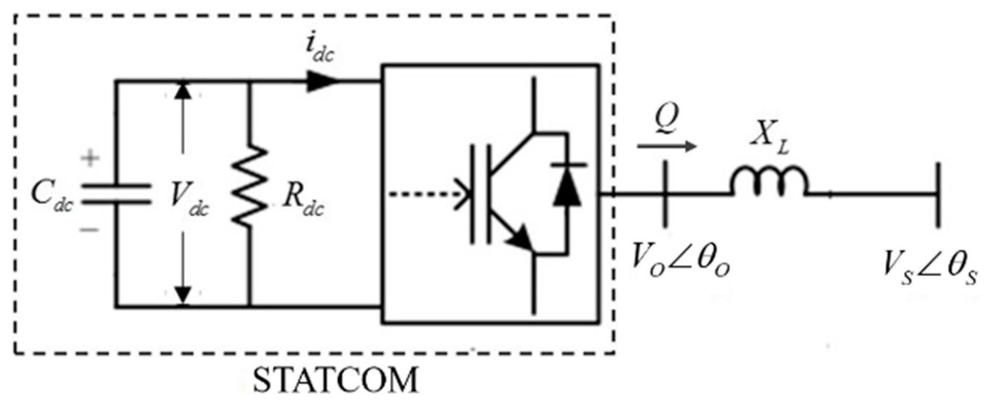
The grid-side voltage can be regulated by adjusting the reactive power flowing on the transmission line (XL) between the STATCOM and the grid buses. Figure 1 illustrates the single-phase STATCOM circuit diagram. Because it requires the phase of the STATCOM output voltage (VO∠θO) and the grid-side voltage (VS∠θS) to be in synchronization, a phase-locked loop (PLL) unit is utilized in the STATCOM control. Equations (1) and (2) represent the real and reactive power of the STATCOM output, respectively, where φ is θO-θS. In this paper, the simulation model of a transmission-level voltage source converter (VSC)-type STATCOM is implemented [27]. The STATCOM includes a 48-pulse and 3-level GTO-type inverter and the related control scheme.
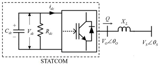
Figure 1.
STATCOM single-phase diagram.
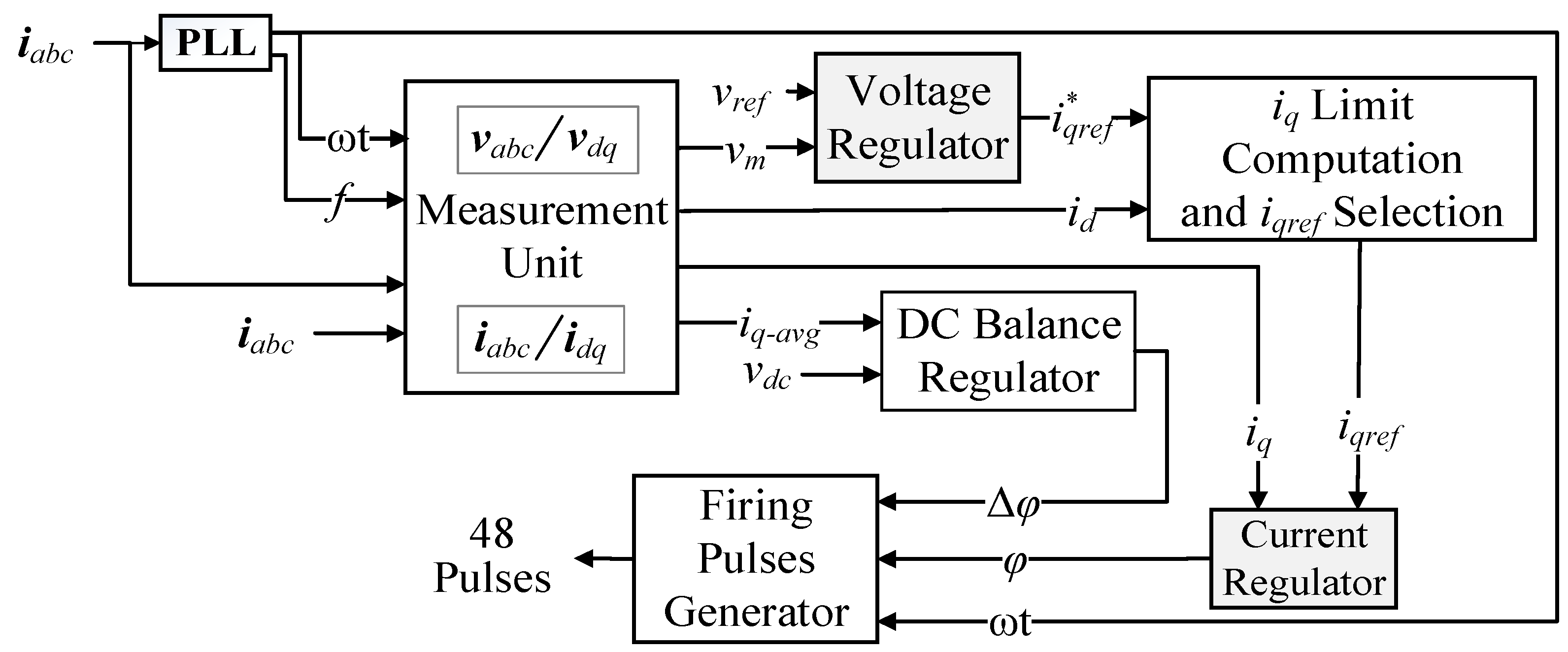
Figure 2 depicts the control block diagram of the GTO-STATCOM. The aim of STATCOM control is to dynamically regulate the capacitor dc voltage to maintain the grid-side voltage. The control scheme includes a PLL module to generate an output signal to the phase detector, which synchronizes GTO pulses to the grid voltage and provides a reference angle, ωt, and system frequency, f, to the measurement unit. The measurement unit then calculates the dq voltage and current components by abc-to-dq reference-frame transformation and outputs the discrete measured voltage, vm = , reactive power, Q, and average d-axis current iq_avg, as well as id and iq. Each of the voltage and current regulators includes a PI controller with two crucial parameters, the proportional (Kp) and integral (Ki) gains, to be adjusted to obtain the desired response of STATCOM. In the voltage regulator, the difference of vm and reference voltage, vref, is determined to obtain the reference reactive current, . In the current regulator, the inputs are iq and iqref and the output is the angle φ, which is the phase shift between the inverter and grid-side bus voltages. The dc balance regulator uses another PI controller, where the positive and negative voltages of the dc-link capacitor are kept equal by applying a small offset, Δφ, on the conduction angles for both half-cycles. The firing pulse generator produces gate pulses for the STATCOM inverter with the inputs of the PLL output, ωt, current regulator output, φ, and dc regulator output, Δφ [27].
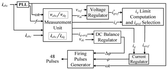
Figure 2.
Control block diagram of STATCOM.
3. Overview of Swarm-Based Algorithms for Optimizing STATCOM PI Controller Gains
The traditional PI controller has been widely applied in various control scenarios. However, different disturbances of output affect the controller performance in practical applications. The traditional PI controller gains are thus difficult to dynamically regulate over time. To overcome this drawback, this paper proposes the Harris Hawks Optimization (HHO)-based PI controller, which can automatically adjust the controller gains under different disturbances when the predefined threshold is triggered. In this study, the PSO, GWO, and KH algorithms are also reviewed and placed under test in order to carry out a performance comparison of the controllers.
3.1. Overview of Harris Hawks Optimization (HHO) Algorithm
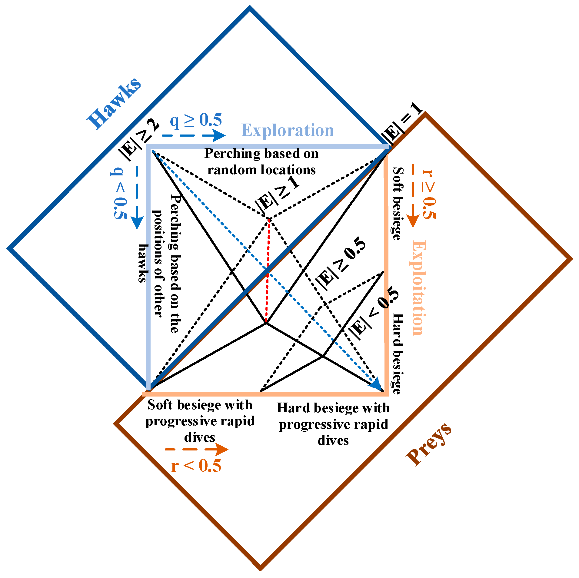
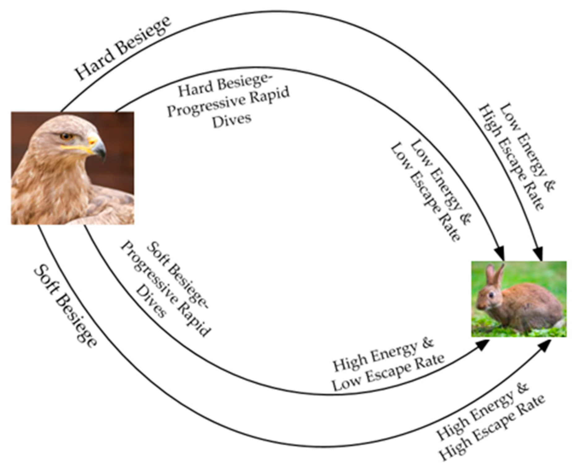
The primary inspiration of Harris Hawks Optimization (HHO) is the collaborative behavior and preying style of the Harris hawk [26]. The Harris hawk hunting operation consists of several eagles hunting prey from different directions and trying to catch them successfully. Based on the escape pattern of the prey (e.g., a rabbit), there are different chasing stages, including exploration, the transition between exploration and exploitation, and exploitation hunting modes, as shown in Figure 3.
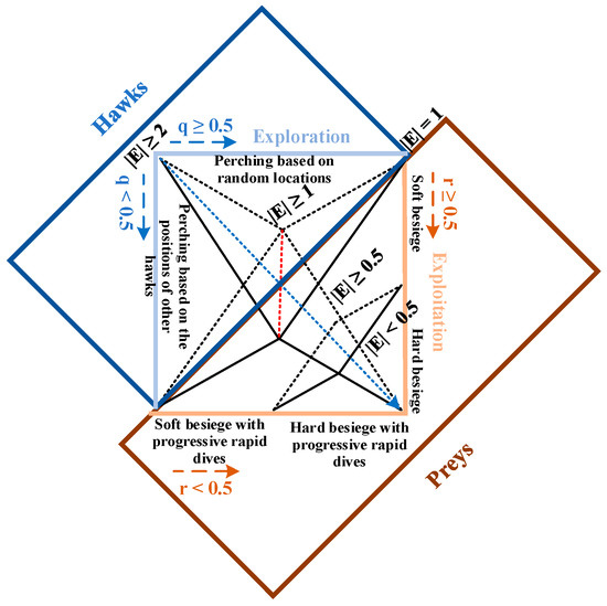
Figure 3.
HHO hunting modes.
3.1.1. Exploration Phase
Harris hawks roost arbitrarily on certain locations (X) and wait to target prey based on the two tactics presented in (3). This step is for the initialization of the solution variables.
where X(t + 1) denotes the vector of position of hawks during the t-th iteration, Xprey(t) represents the prey position. r1, r2, r3, r4, and q are random values between 0 and 1. LB and UB are the variable’s lower and upper bounds, respectively. Xrand(t) is a random variable (i.e., the hawk) chosen from the present population. Xm is the average of the positions of the present population of hawks and is calculated using
where Xi(t) is the i-th hawk’s location during iteration t and N represents the overall number of hawks (i.e., agents).
3.1.2. Transition from Exploration to Exploitation
During this stage, the escaping energy of the prey is defined as follows.
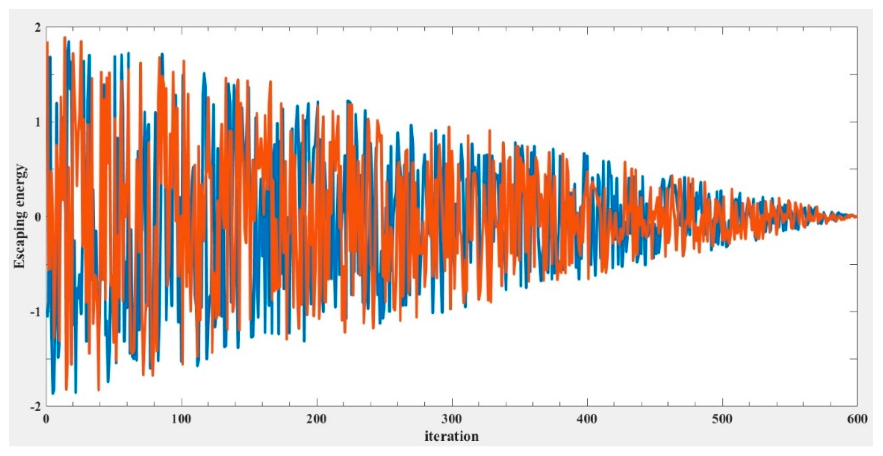
where t is the iteration index, T is the maximum iteration number, E0 is the initial energy of the prey. The behavior of E over time can be illustrated using Figure 4. As the iteration number increases, the escaping energy gradually declines. Figure 5 illustrates the Harris hawk predation patterns during exploitation [25], which will be described in the following sections.

Figure 4.
Escaping energy variation trend during two runs in 600 iterations.

Figure 5.
Predation patterns during exploitation of the HHO algorithm.
3.1.3. Exploitation Phase: Soft Besiege
During this stage, the variable (position) is updated by
where ΔX(t) denotes the difference between the current location and the position vector of the prey. J = 2 × (1 − r5) defines the arbitrary jump endurance of the prey in the escaping energy of (5) and changes arbitrarily during each iteration. r5 is a random number selected from [0, 1].
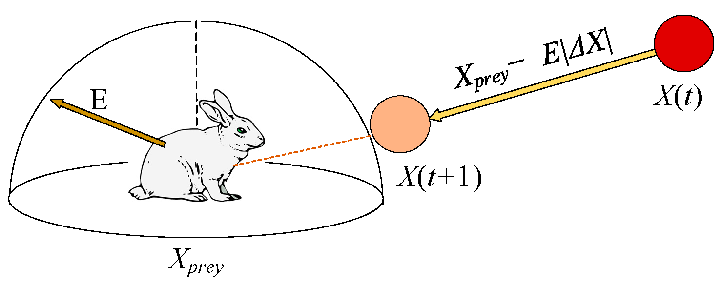
3.1.4. Exploitation Phase: Hard Besiege
In this stage, the position is modeled by
A graphical illustration of this stage with one hawk is shown in Figure 6.

Figure 6.
Example of overall vectors in hard besiege case.
3.1.5. Exploitation Phase: Soft Besiege with Progressive Rapid Dives
For the soft besiege, the hawks are assumed to update the next step (i.e., movement) following (9).
The hawks dive according to the levy flight function (LF)-based forms of
where D is the problem dimension. S is a 1 × D random vector and LF is the levy flight function calculated by
where
where β is 1.5, u and v are two random values within [0, 1]. Γ(•) is the gamma function. Therefore, the evaluating positions of hawks are performed by
where F(•) is the fitness function. A graphic illustration for this step with one hawk is depicted in Figure 7 [26].
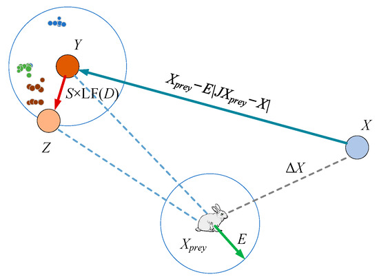
Figure 7.
Vectors in illustrative soft besiege with progressive rapid dives.
3.1.6. Exploitation Phase: Hard Besiege with Progressive Rapid Dives
The rule listed below relies on the hard besiege scenario.
where Y′ and Z′ are defined by the updated rules below.
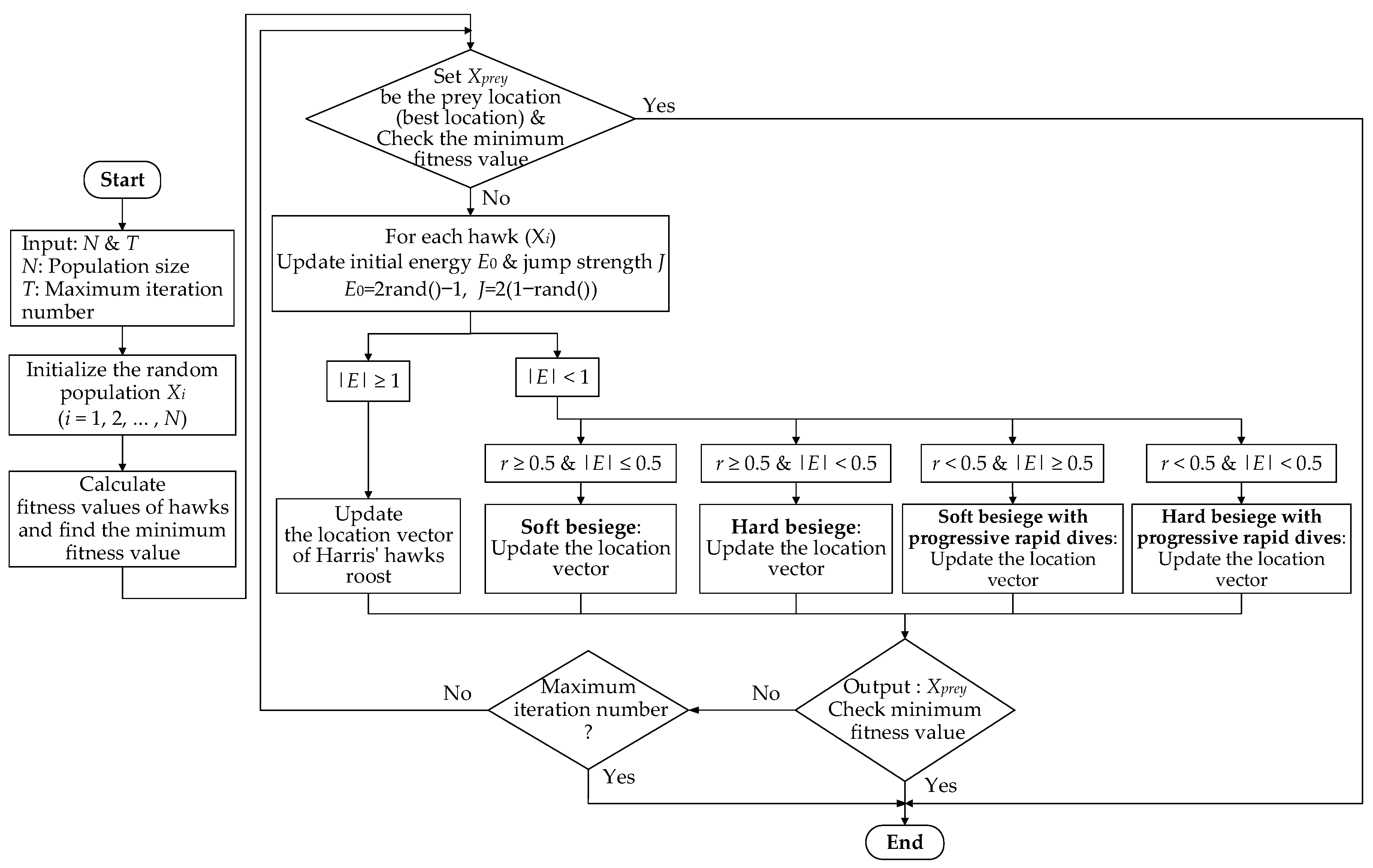
Figure 8 depicts the flowchart of the HHO algorithm. The first part is parameter setting. In HHO, each potential solution is classified based on the escaping energy of E and r without surviving by any situation or probability, and different operations (i.e., besiege) are performed. Therefore, for each potential solution, only one besiege is executed, which can reduce the solution time substantially. The besiege categories are divided into four strategies and a direct output option. The method can lower the iteration number, and the algorithm converges faster than other compared swarm-based algorithms.
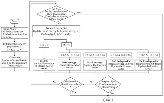
Figure 8.
Flowchart of the HHO algorithm.
Major steps of the HHO algorithm for obtaining the optimal PI controller gains are as follows.
- Step 1. Set the number of variables (D), population sizes (N), and maximum iteration number. Let Xprey be the prey (i.e., the best location).
- Step 2. Initialize the Harris hawks location X.
- Step 3. Calculate the fitness value (i.e., objective function value) of Harris hawks F(X).
- Step 4. Update the prey location Xprey and its fitness F(Xprey).
- Step 5. Compute the escaping energy E of the prey using (5).
- Step 6. Update the Harris hawks location Xi, i = 1, 2, …, N, based on the value of E. If |E| ≥ 1, execute (3); if |E| < 1, perform the exploitation phase using the four strategies.
- Step 7. Calculate the new fitness value F[Xi(t + 1)] as in Step 3.
- Step 8. Check the new fitness value and its previous one. Then, update the fitness value according to the following rule:
If F[Xi(t + 1)] < F[Xi(t)], let F[Xi(t)] = F[Xi(t + 1)] and Xi(t) = Xi(t + 1).
Otherwise, retain the old fitness value.
- Step 9. Check if the maximum number of iterations is reached. If yes, stop and output the optimal solution, Xprey, (i.e., optimal controller gains); otherwise, return to Step 4.
3.2. Particle Swarm Optimization (PSO)
The idea of particle swarm optimization (PSO) is to conduct a large-scale search operation with the unit of a particle. It can also be imagined with reference to animals such as flocks of birds or schools of fish. These swarms conform based on a specific method to find food, and each individual keeps changing their search pattern according to their learning experiences [28].
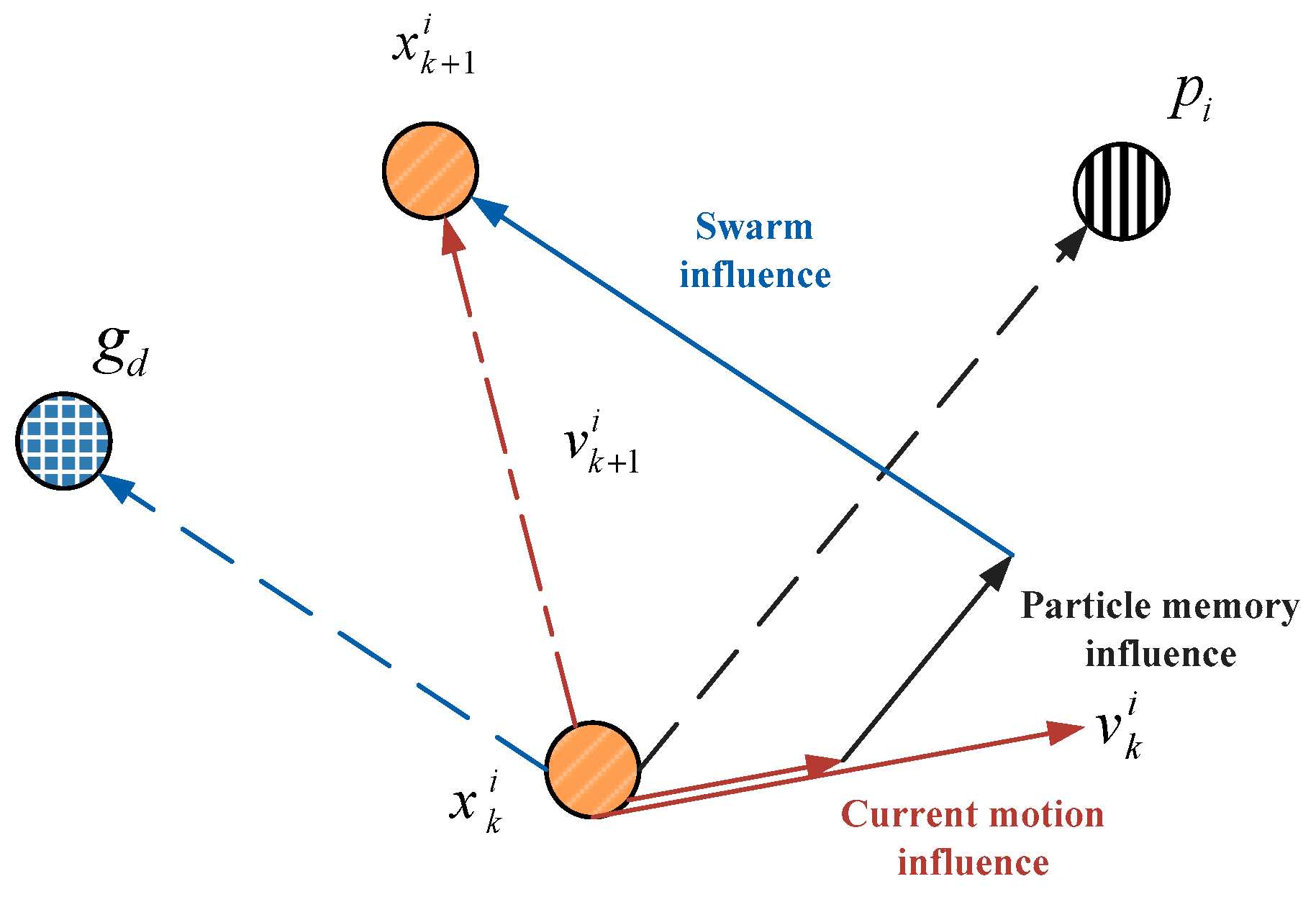
In the PSO algorithm, the problem’s feasible solution is represented by the particle’s position in the solution space. Each member within the population is defined as a particle and the population is defined as a swarm. Each particle refers to a possible optimal solution and has a velocity vector that governs its moved direction and speed. Therefore, individual position is updated by tracing individual and global optima in the search space. The fitness value is computed if the individual position is renewed. The position associated with the best fitness is known as pbest, and the overall best out of all the particles in the population is defined as gbest. Through comparison the fitness of the new particle with the optimal individual and global ones, the positions of the individual and global optima are updated. The essential PSO algorithm is depicted in Figure 9. The particle’s position and speed are updated by (17) and (18).
where w is the inertia weight; and are the i-th particle’s velocity and position during the (k + 1)-th iteration, respectively; and are learning factors; and are two random numbers within [0, 1]; and denote the individual optimum (pbest) and the global optimum (gbest), respectively.
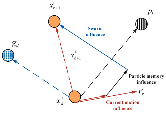
Figure 9.
Illustration of the velocity and position updates in PSO.
The following summarizes the major steps of the PSO procedure for searching optimal parameters.
- Step 1. Set the population size and initialize each particle’s position and velocity vectors (i.e., controller gains) randomly.
- Step 2. Compute each particle’s fitness value.
- Step 3. Compare the particle’s fitness value with the individual optimum (pbest).
- Step 4. Find the best of all particles and compare the fitness value with global optimum (gbest).
- Step 5. Update each particle’s velocity and position according to (17) and (18). Return to Step 2 until the maximum iteration number is achieved.
- Step 6. Obtain the optimal solution (i.e., controller gains).
3.3. Overview of Grey Wolf Optimization (GWO) Algorithm
The GWO algorithm simulates the predation and hunting performance of grey wolves [29]. The GWO procedure includes the grey wolf’s social hierarchy system, encircling, and hunting, as described below.
3.3.1. Social Hierarchy
There is a social hierarchy system between the wolves, and each individual in the group has a clear division of labor and cooperation. As depicted in Figure 10, the social hierarchy of wolves is separated into α, β, δ, and ω. In the algorithm, each level of the wolf pack represents each wolf’s fitness. Among them, the three grey wolves with the best fitness values are denoted as α (the value closest to the best solution), β, and δ, respectively, and the rest of the wolf pack are ω.
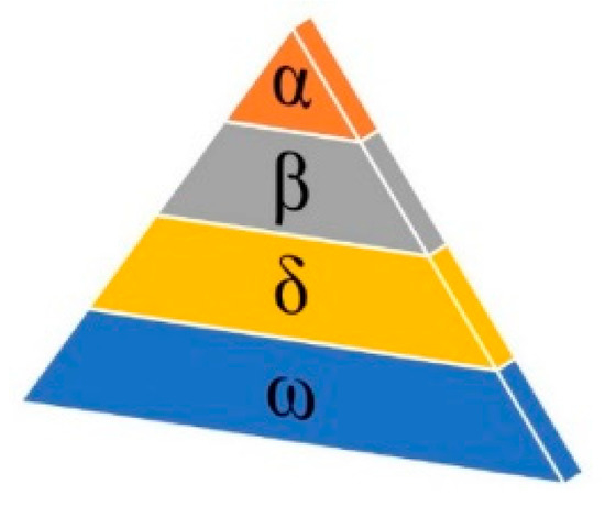
Figure 10.
Grey wolf social hierarchy.
3.3.2. Encircling Prey
After finding the prey’s position, the wolves must firstly encircle the prey. During this process, the distance between the grey wolf and the prey can be stated by (19) and (20), respectively.
where D is the distance between the wolf and the prey, t is the present iteration, X(t) is the position of the wolf (i.e., the potential solution), and Xp(t) is the prey’s position (i.e., the optimal solution). a = 2kr1 − k and c = 2r2 are coefficients, where k decreases linearly from 2 to 0 as the number of iterations increases; r1 and r2 are two random numbers within [0, 1].
3.3.3. Hunting
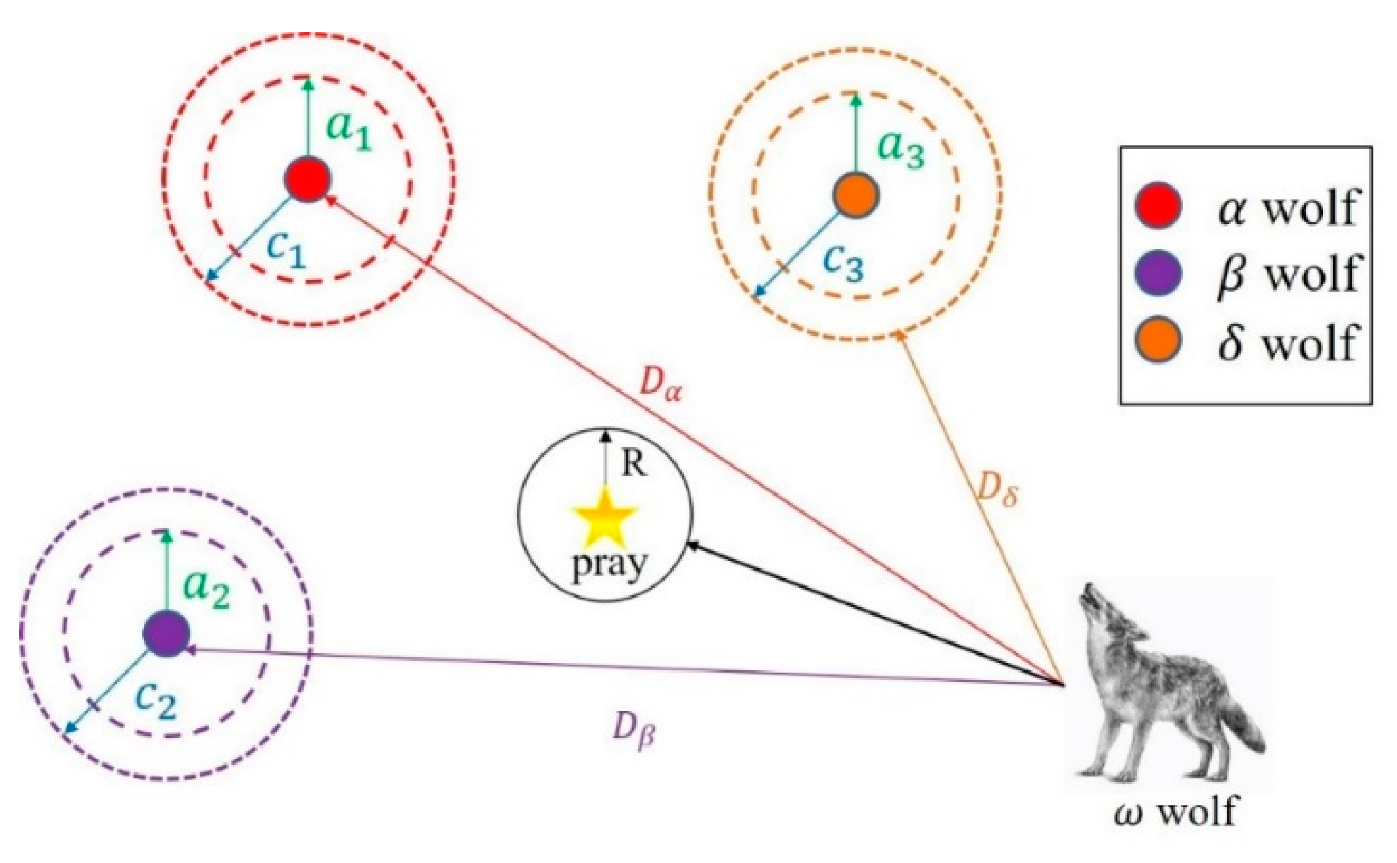
After encircling the prey, the β and δ wolves will hunt the prey under the guidance of the α wolf. During hunting, the position of the ω wolves will change with the escape of the prey, and the prey’s position will be relocated based on the current position of α, β, and δ wolves. The mechanism by which the wolves update their positions is illustrated in Figure 11. The update equations are shown in (21).
where c1, c2, and c3 are random disturbances; Xα, Xβ, and Xδ denote the current positions of α, β, and δ wolves; Dα, Dβ, and Dδ are the distances between α, β, and δ with respect to the ω wolves; X represents the present position of the wolf. The final position of ω wolves is defined in (22).
where , , and .
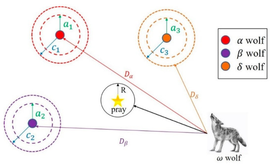
Figure 11.
Position update in GWO algorithm.
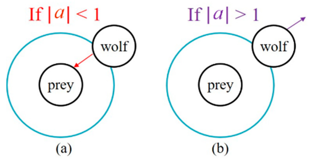
The GWO algorithm emphasizes the function of exploration by checking if |a| is greater than one or not to change the direction of the grey wolf and enhance the exploration ability, as shown in Figure 12. The coefficient factor “a” changes in [−k, k] along with the value of “k”, which declines linearly from 2 to 0 during the iteration processes. When |a| is larger than one, GWO conducts a global search and goes away from the current prey. The coefficient factor c is another parameter that directly affects the grey wolf algorithm. In (21), c is a random value between 0 and 2 and is linearly decreasing. The parameter C enhances the solution search ability during the iterative procedure when the solution traps in the local optimum.

Figure 12.
GWO search directions: (a) attacking prey; (b) searching for prey.
Major steps of GWO algorithm for searching optimal parameters are summarized below.
- Step 1. Initialization of parameters. Set the grey wolf number in the group and the maximum iteration number.
- Step 2. Calculate each wolf’s fitness value.
- Step 3. Sort the fitness values obtained at Step 2. Then, find the top three individuals with minimum values and assign them as α, β, and δ, respectively.
- Step 4. Update the wolf positions using (19)–(22).
- Step 5. If the maximum iteration number is achieved, the algorithm terminates. Output the results of the present position which represents the optimal solution (controller gains). Otherwise, return to Step 2.
3.4. Overview of Krill Herd Algorithm
The krill herd (KH) algorithm simulates krill swarms responding to certain environmental and swarm processes [30]. The herding of the individual krill includes two major goals: (1) increasing the density of krill herd, and (2) reaching food. The fitness function of each individual krill is denoted as the distance between the highest density of the swarm and the food. The time-varying position of an individual krill in the two-dimensional surface is governed by (23).
where Ni is the movement performed by other individual krill, Fi is the foraging activity, and Di is the random diffusion. Next, these three factors are introduced one by one.
3.4.1. Motion Induced by Other Individual Krill, Ni
For an individual krill, this movement is governed by
where
Nmax is the maximum induced speed, ωn is the inertia weight within [0, 1] of the motion induced, is the previous motion induced, is the local effect associated with the neighbors, and is the aim direction effect contributed by the best individual krill. In the study, the neighbor effect on an individual krill’s movement is calculated by (26)–(28).
where Kbest and Kworst are the individual krill’s best and worst fitness values so far; Ki is the fitness function value of the individual krill; Kj represents the fitness value of the neighbor; X is the associated positions; and NP is the number of neighbors. To avoid singularities, a minor positive number, ε, is included in (28).
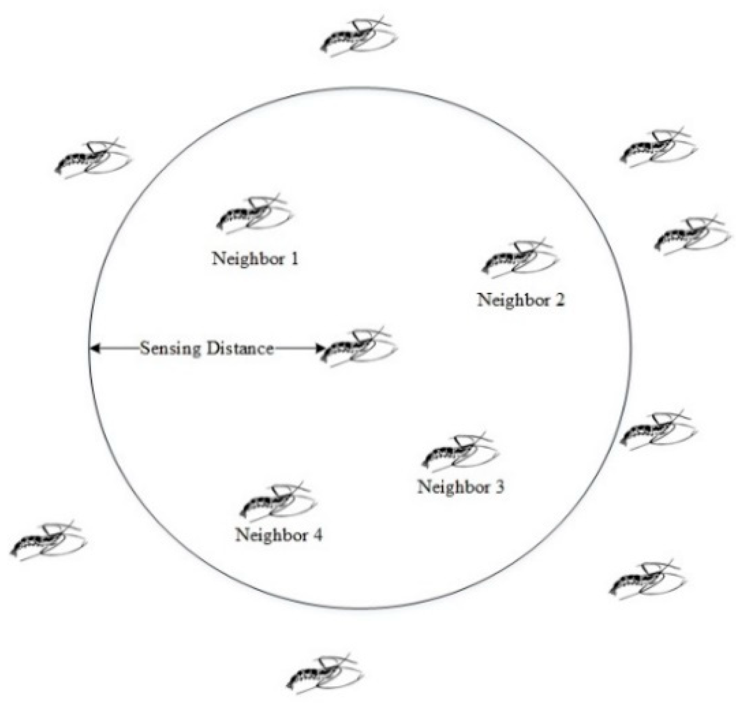
Equations (26)–(28) include certain unit vectors and normalized fitness values. The vectors indicate the induced directions by the other neighbors and each value implies the contribution of a neighbor. The vector of the neighbors can be either attractive or repulsive, since the normalized value can be either positive or negative. There are many strategies to be used for choosing the neighbor. For instance, ref. [30] proposes a method that is a neighborhood ratio defined to search for the closest individual krill. Using the individual krill’s actual behavior, a sensing distance is computed around an individual krill, as depicted in Figure 13.
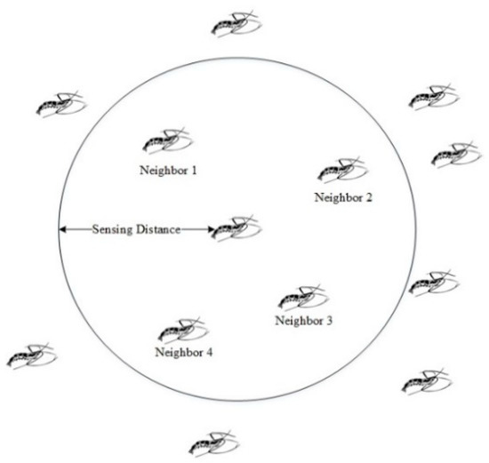
Figure 13.
Sensing ambit around an individual krill.
The sensing distance of each individual krill is assessed using different heuristic approaches. Here, we determined to use (29) for each iteration to specify the krill as the center and plot a circle with the radius same as the sensing radius. If there are other krill in this circle, they are regarded as neighbors with the center krill.
where ds,i is the individual krill sensing distance and NP is the krill number. The factor of 5 is based on numerical experience.
An individual krill’s target vector is the smallest fitness value of the individual krill. Through (30), the krill is derived to the global optimal state by calculating the influence of the global optimum krill and the current optimal krill direction.
where Cbest is the effective coefficient of the individual krill possessing the best fitness value to the i-th individual krill. The value of Cbest is defined below.
where rand is a random value within [0, 1] and is for enhancing exploration, t is the iteration number, and tmax is the maximum iteration number.
3.4.2. Foraging Motion, Fi
The foraging motion consists of two major parameters. The first is the current food location and the second is the previous food location. This motion can be expressed by
where
Vf is the foraging speed, ωf is the inertia weight within [0, 1] of the foraging motion. In the last foraging motion, is the food attractive, and represents the effect of the krill’s best fitness value so far.
In this study, the virtual center of the food concentration is assessed based on the fitness distribution of the individual krill. The food center for each iteration is given by
The food attraction for the individual krill is found using (35) as follows.
where Cfood defines the food coefficient. Because the food effect in the krill herding reduces during the time, Cfood is thus calculated using
The best fitness effect of the individual krill is also determined by (37).
where is the best position previously visited by the individual krill.
3.4.3. Physical Diffusion, Di
Physical diffusion of individual krill is regarded as a stochastic process, which is formulated by (38).
where Dmax denotes the maximum diffusion speed, and δ represents the random directional vector and its arrays include random values within [−1, 1]. The better the position of the krill, the minor the randomness of the movement. Therefore, the effects of the motion induced by other individual krill and foraging motion progressively decline with increasing the iteration number. Equation (38) then can be rewritten by (39).
Through three main parameters described above, each krill’s velocity of is computed. The updated position of each krill is expressed by
where Δt denotes the velocity effect on the new position of the krill. Since this parameter is adjusted by the search space, Δt can be expressed by (41).
where NV is the number of total variables, and LBj and UBj represent lower and upper bounds of the j-th variable, respectively. Therefore, the difference of the two bounds shows the search space. Ct is a number varying within [0, 2]. It is also obvious that low values of Ct cause the individual krill to search thoroughly in the solution space.
The following steps are performed to adjust the PI controller parameters based on the KH algorithm.
- Step 1. Initializion of parameters. Set the number of the krill herd and the maximum iteration number. Ensure that their production positions are within the feasible range.
- Step 2. Compute each individual krill’s fitness value. Prioritize the fitness value of each individual krill and determine the krill’s position.
- Step 3. Motion induction setting. The neighbors of the individual krill are identified by (29), and the neighbor inducibility is determined by (26)–(28). The induction of the optimum krill for the present krill is obtained using (30).
- Step 4. Foraging motion setting. In the foraging movement, “food” is an “ideal best point”, and the virtual food position is obtained by (34). The influence of food on individual krill is determined according to (32) and (33).
- Step 5. Random diffusion setting. Through Steps 2 and 3, the krill particles’ positions are known. The better the position is, the lower the probability of random diffusion of the particles is. This step is mainly to spread the poorly located particles to other positions by diffusion motion.
- Step 6. Finding the optimal individual krill. Each krill can evaluate the individual’s quality through the fitness function value and obtain the best particle. The update rule is governed by
If , remains unchanged; otherwise, .
represents the fitness function value corresponding to the particle group at the i-th iteration.
- Step 7. Return to step 2 until the maximum iteration number is achieved. After the iteration ends, output the optimal krill individaul (i.e., controller gains).
4. Implementation of Swarm-Based Algorithm in STATCOM PI Controllers
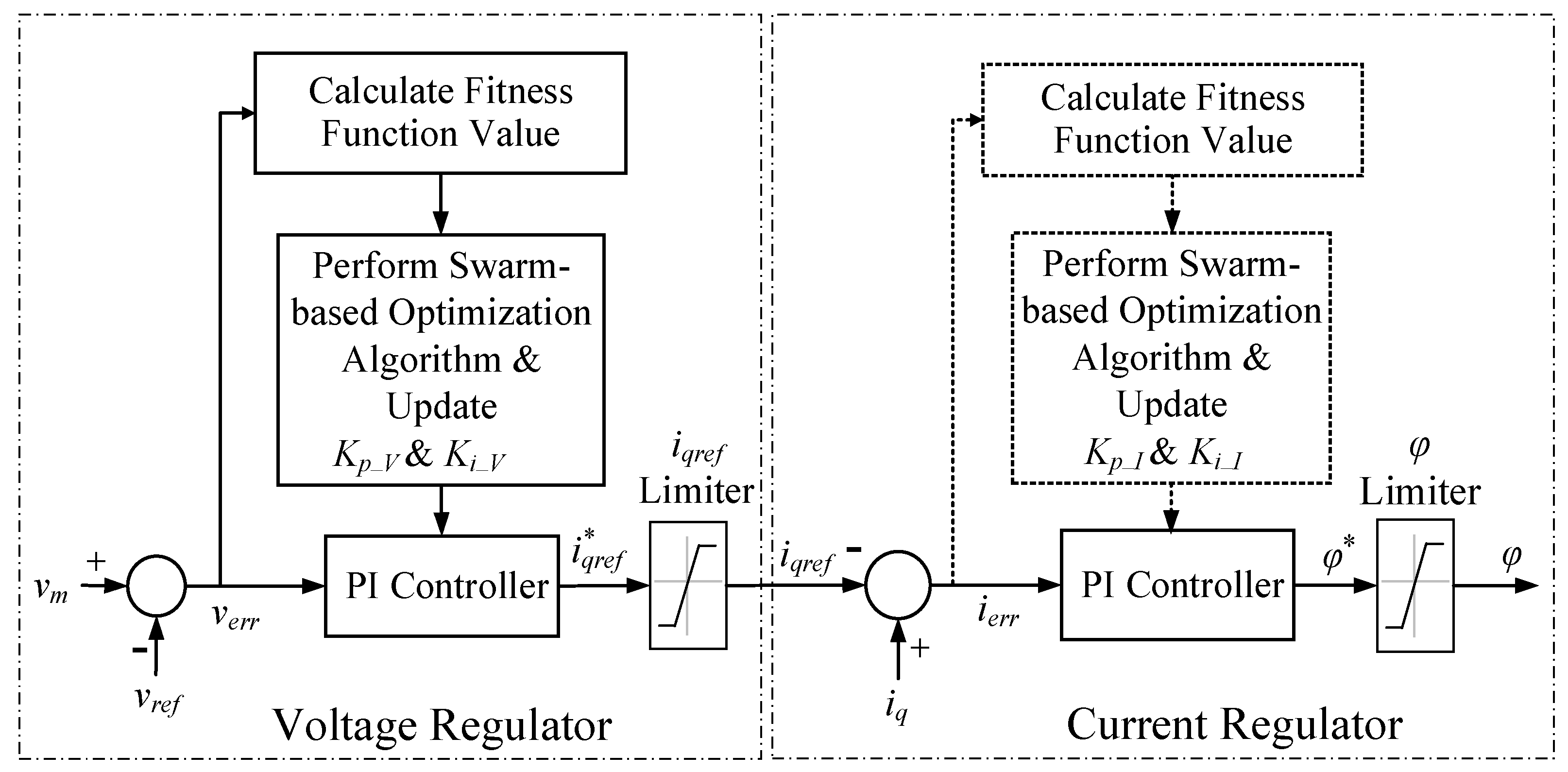
In the block diagram of the STATCOM control in Figure 2, the ac voltage and current regulators are implemented with PI controllers. In the traditional method, the controller gains Kp and Ki are fixed, which are not suitable for maintaining the STATCOM terminal voltage due to drastic reactive power-consumed loads or variations in renewables output. To tackle such challenges, Figure 14 presents an adaptive PI controller combined with the swarm intelligence-based adjustor for PI controller gains. The controller gains GTO-STATCOM voltage regulator can be self-adjusted under different wind farm output variations.

Figure 14.
The proposed HHO-based PI controllers of STATCOM voltage and current regulators.
4.1. Swarm Intelligence-Based Adjustor for PI Controllers
In Figure 14, the controller input is the difference between the reference and the measured STATCOM bus voltage values. This error signal is processed by the PI controller and output angle φ, which is provided to the signal generator. The gain adjusters are also drawn. It is significant that Kp_V and Ki_V are produced by the adjustor through the error voltage signal, verr, as the input. After that, this set of parameters will be sent back to PI controller to calculate the optimal reactive reference current, , using (42), and go through the reference current limiter to input the final reference current, iqref, to the current regulator. The inclusion of swarm-based PI controller for calculating Kp_I and Ki_I of the current regulator is also illustrated within the dashed line block for additional comparison purpose; otherwise, it will be the classic PI controller in the study. Then, the optimal phase angle (φ*) in the current regulator is calculated using (43) and output the final angle, φ, through the angle limiter.
The PI controller gains, Kp and Ki, are used in the voltage and current regulators. The reference reactive current signal () and phase angle (φ*) used for the firing pulse generator of the converter shown in Figure 2 are calculated at each sampling time step, as given in (42) and (43), respectively. These two parameters are dynamically updated over time for STATCOM terminal voltage regulation.
where TS is the sampling time and verr is the difference between the measured voltage, vm, and the reference voltage, vref. The phase of the STATCOM inverter voltage referred to the connected grid bus voltage is φ.
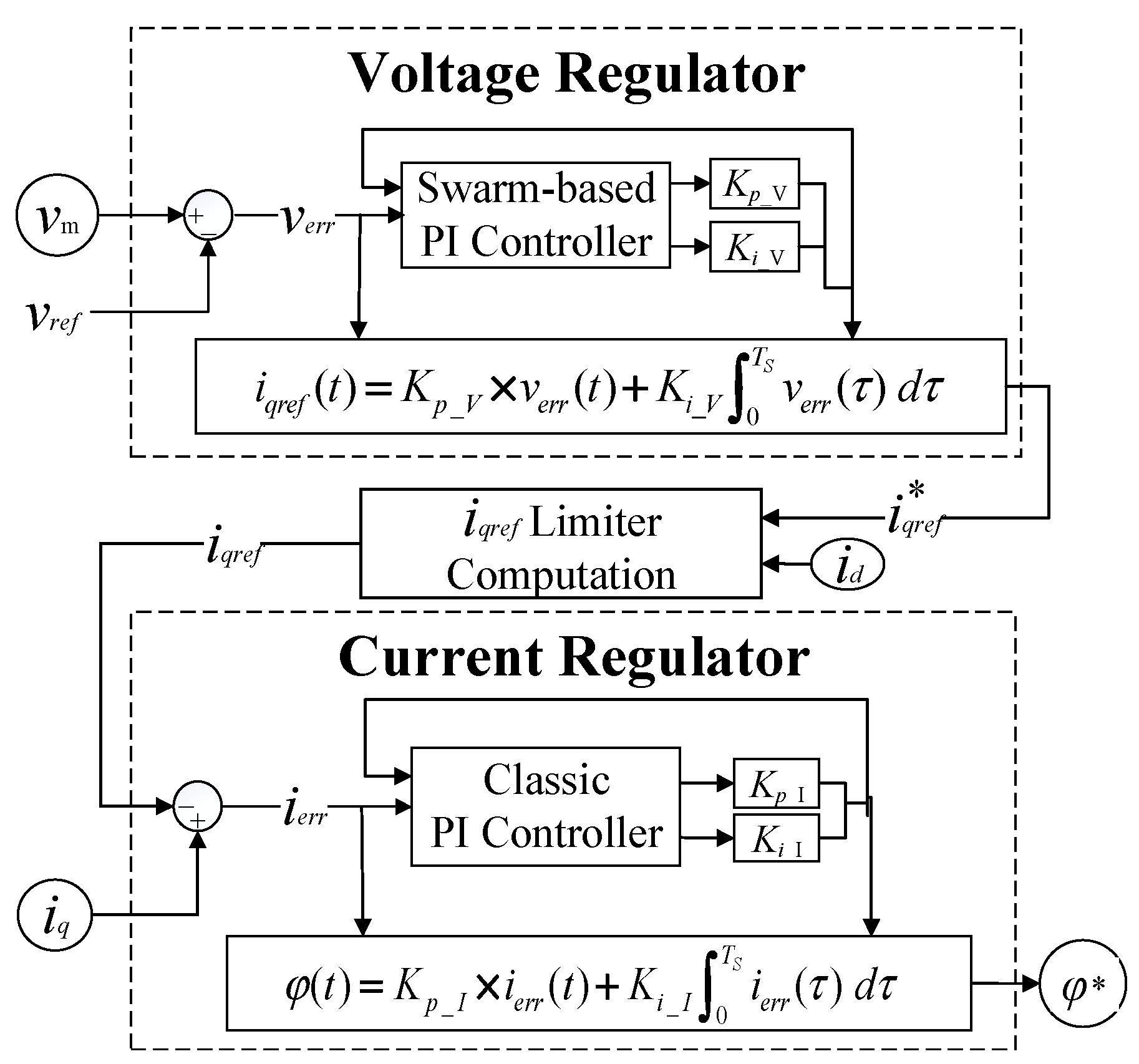
Figure 15 shows the schematic diagram of GTO-STATCOM voltage and current regulators. A module of the reactive current limiter (iq Limit Computation) is between these two regulators. The middle of the model determines a more suitable value of iqref by id, and then sends it to the current regulator. The angle φ* is output to the angle limiter and then the angle φ is output to the converter to determine the firing pulses required to mitigate the voltage fluctuation at the STATCOM terminal bus.
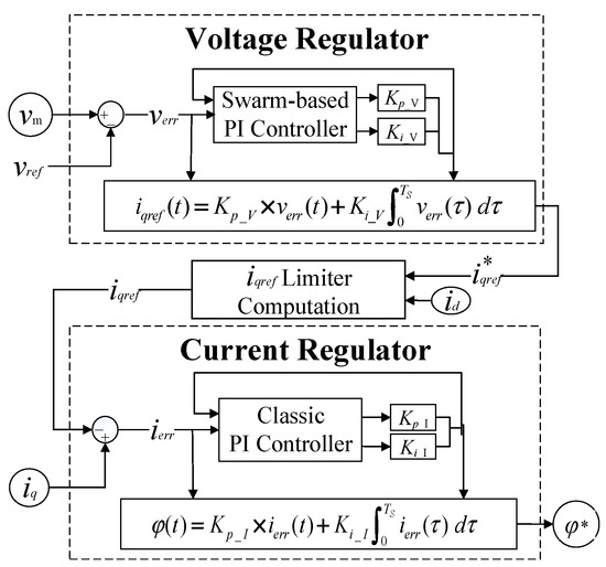
Figure 15.
STATCOM voltage and current regulators with swarm-based PI controller.
4.2. Swarm-Based Algorithm Implementation for PI Controller of STATCOM Voltage Regulator
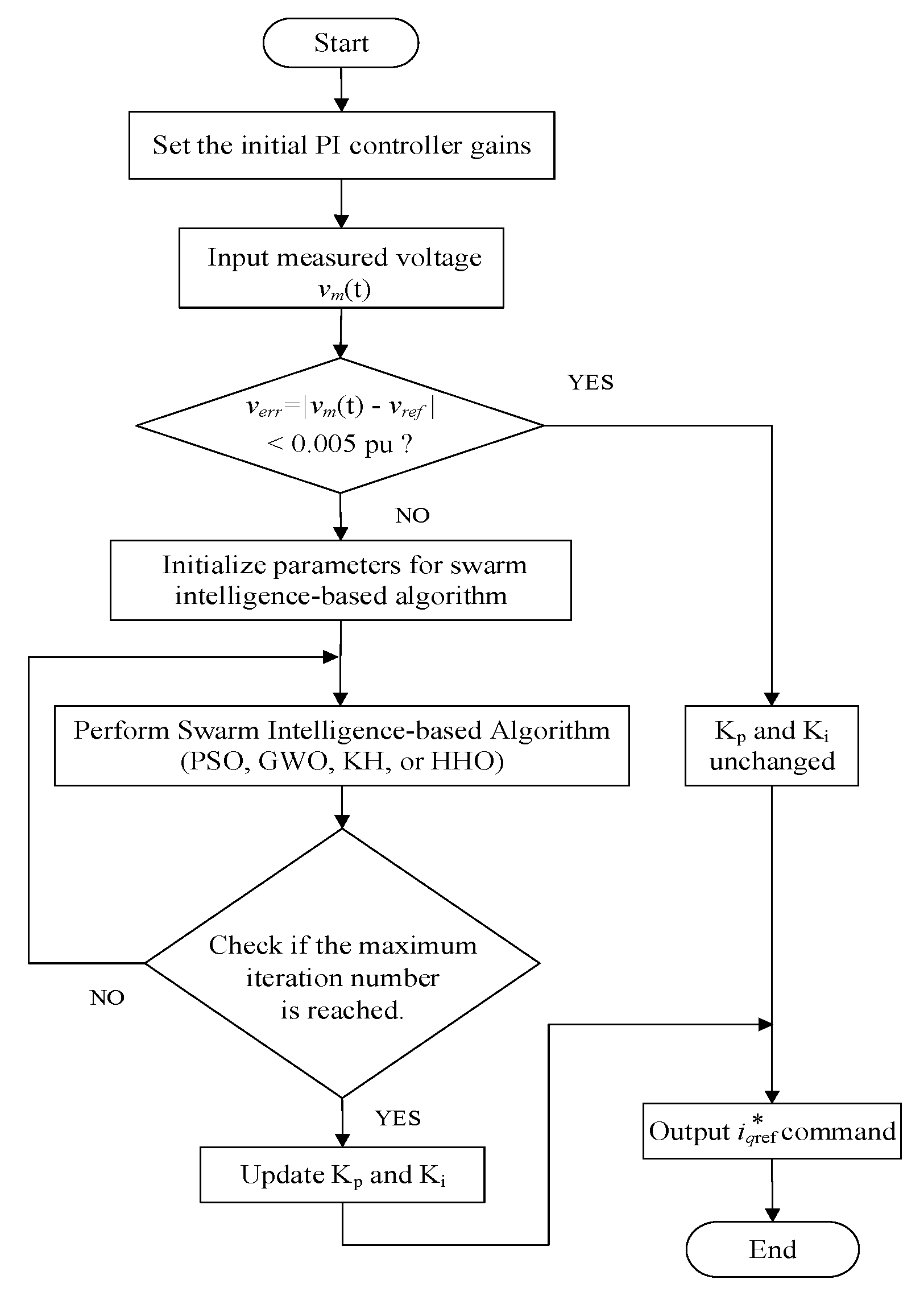
In controller gains calculation using swarm-based optimization algorithms, the fitness function (i.e., objective function) for each sampling time step, TS, uses the trapezoidal rule and is defined in (44).
Begin with the initial time step; the procedure runs until the difference (i.e., verr) of the measured STATCOM terminal bus voltage and its reference (i.e., 1 p.u.) is less than 0.005 p.u. or the iteration number reaches to its limit. The swarm-based PI controller of the current regulator is implemented in the same manner. Figure 16 depicts the solution flowchart for the calculation of optimal PI controller gains.

Figure 16.
Flowchart of the proposed swarm intelligence-based algorithms for optimizing PI controller gains.
5. Results
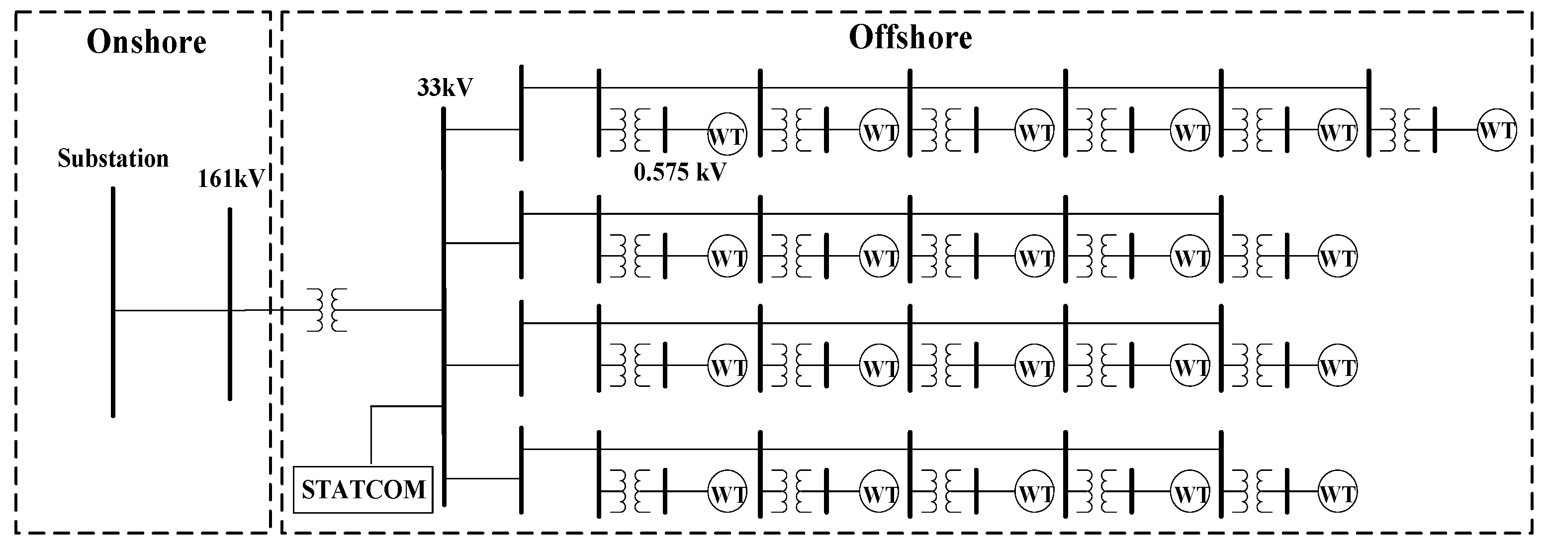
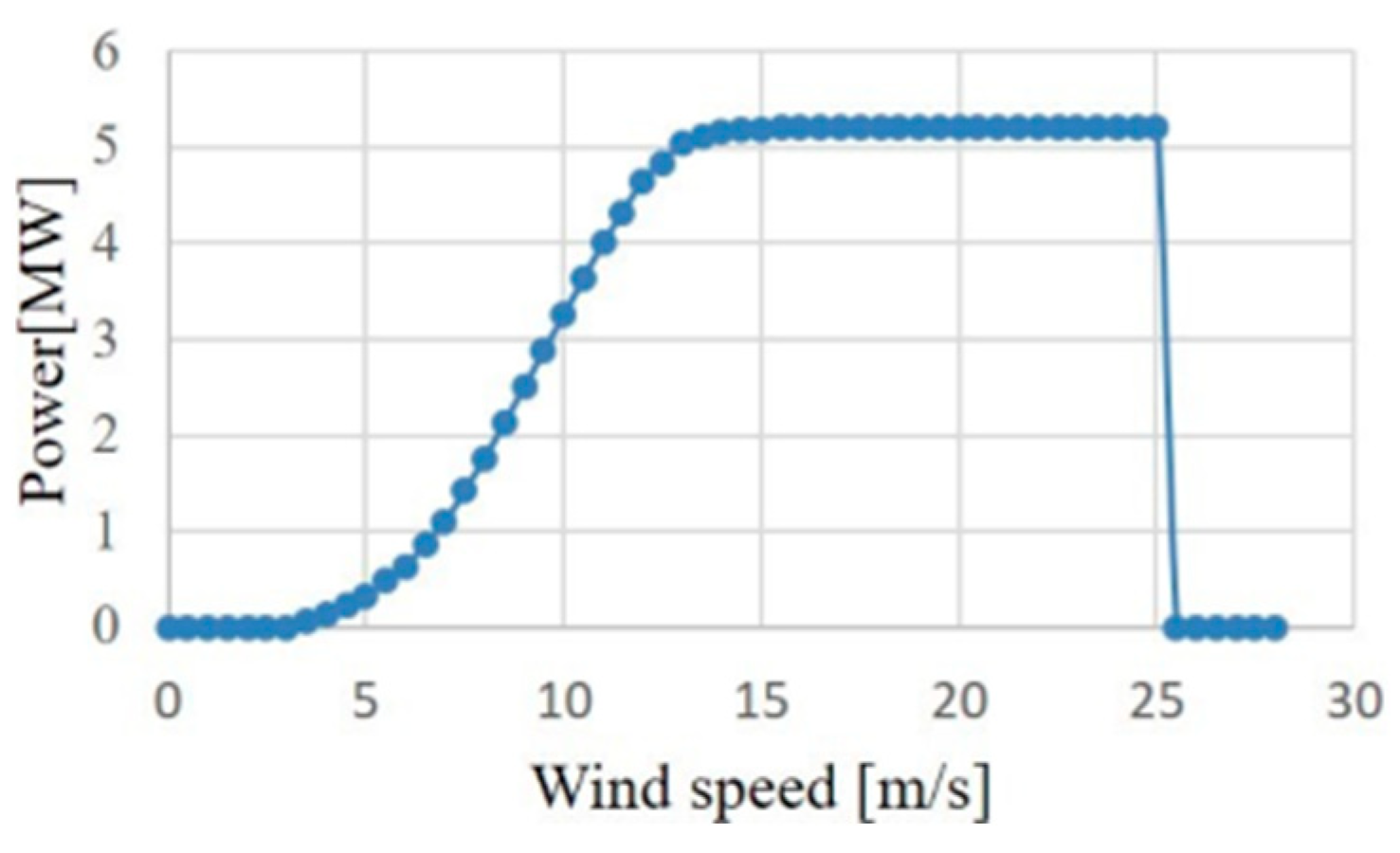
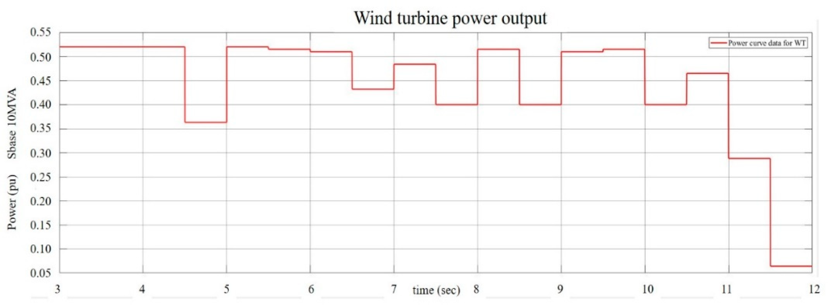
To show the usefulness of the swarm intelligence-based algorithms for obtaining the optimal PI controller gains of GTO-STATCOM voltage regulator, simulation results for mitigating the voltage fluctuation at STATCOM terminal bus that connects an offshore wind farm are reported. Figure 17 depicts the actual offshore wind farm and STATCOM system under study, near the west coast of central Taiwan. Figure 18 shows the study system implemented by MATLAB/Simulink. The study system includes 21 WTs at a capacity of 5.2 MW each, a 140 MW load, and a 30 MVAr STATCOM connected to the 33 kV bus for complying with the grid code requirements [31]. In the study, the measured hourly average wind speed in one day is converted to a sequence of equivalent 12-s-long data and these are input to the lookup table corresponding to each WT power curve, which converts the wind speed into active power output. Figure 19 and Figure 20 show the output power versus wind speed curve of each WT and the one-day equivalent power output of the WT under study. Table 1 lists the adjustment parameters of the four compared swarm intelligence-based algorithms and Table 2 provides the STATCOM system parameters.

Figure 17.
Single-line diagram of the offshore wind farm and STATCOM system under study.
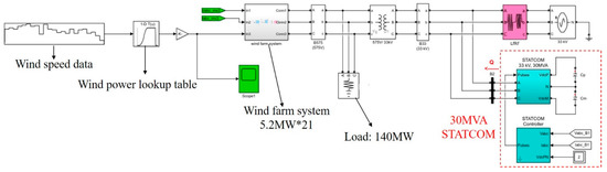
Figure 18.
Simulink circuit model of the studied system.
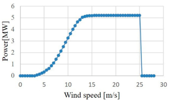
Figure 19.
Wind speed vs. power output curve of a 5.2 MW wind turbine.
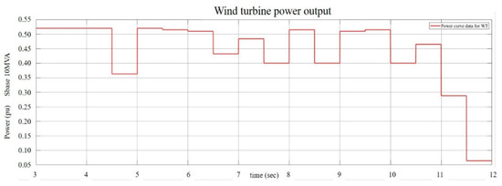
Figure 20.
One-day equivalent power output of the wind turbine.

Table 1.
Parameters of four swarm intelligence-based optimization algorithms.
Table 2.
Parameters for GTO-STATCOM system under test.
In the simulation, two study cases are reported. The first case is to test the STATCOM compensation performance using the proposed HHO and the compared algorithms of PSO, GWO, and KH. The wind turbine output variation of the wind farm for the first case is as shown in Figure 20. Voltage at the 33 kV bus with and without STATCOM compensation obtained by the four algorithms are depicted in Figure 21. The second case is to test the compensation performance under four different degrees of the wind power output variation with and without STATCOM compensation obtained by implementing GWO and HHO in the PI controller of STATCOM voltage regulator. The STATCOM terminal voltages at the 33 kV bus with and without STATCOM compensation for the second case are shown in Figure 22.
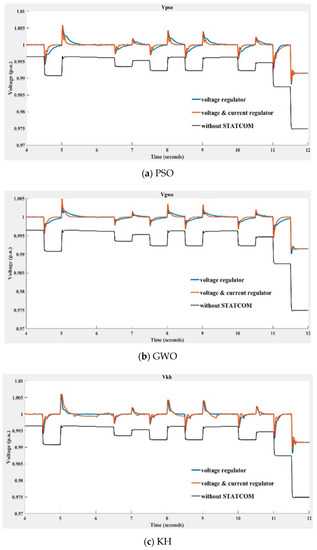
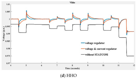
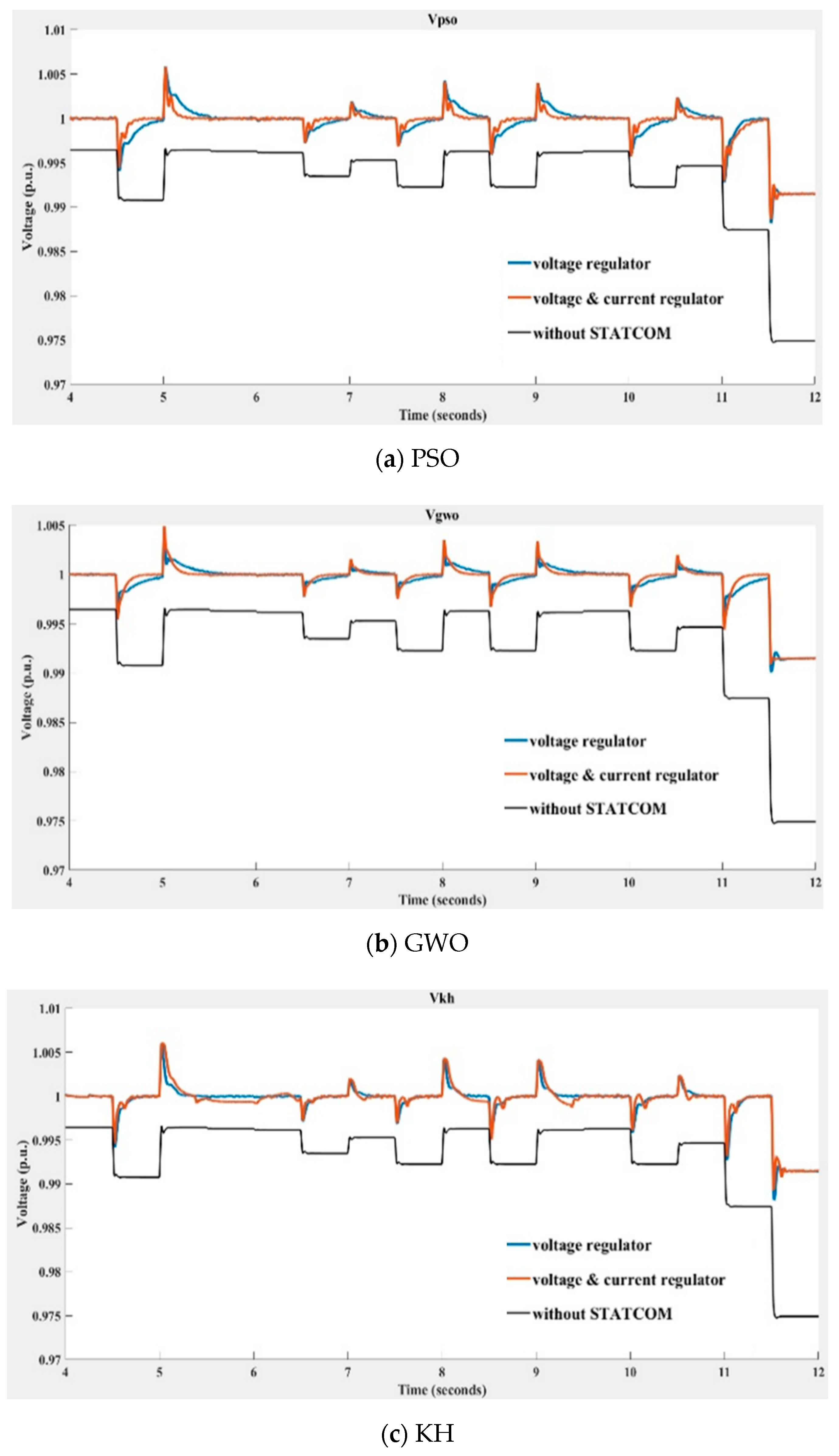
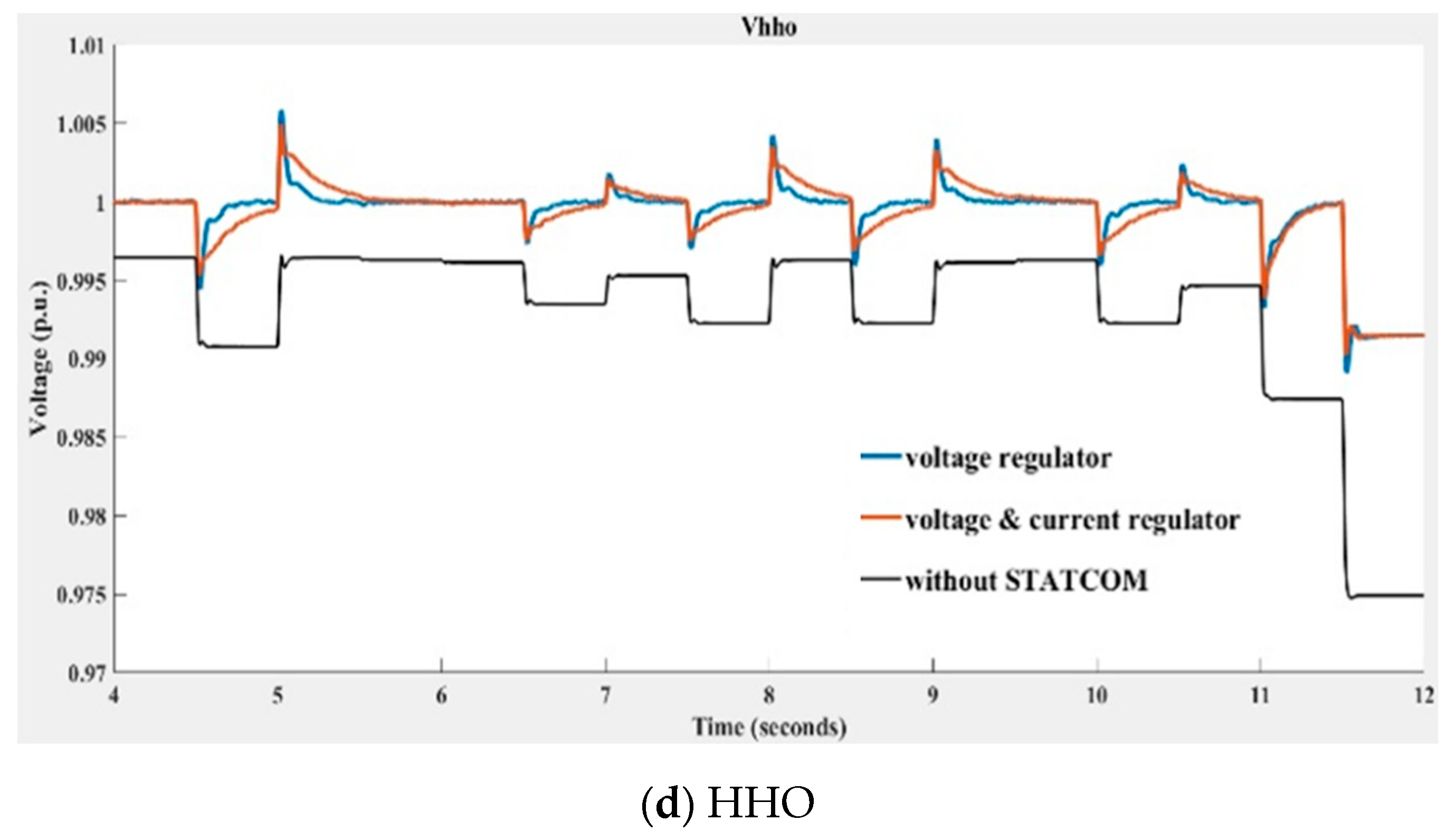
Figure 21.
Voltage at the 33 kV bus with and without STATCOM compensation obtained using (a) PSO, (b) GWO, (c) KH, and (d) the HHO algorithms (blue line: swarm-based voltage regulator and classic current regulator; orange line: swarm-based voltage and current regulators; black line: without compensation).
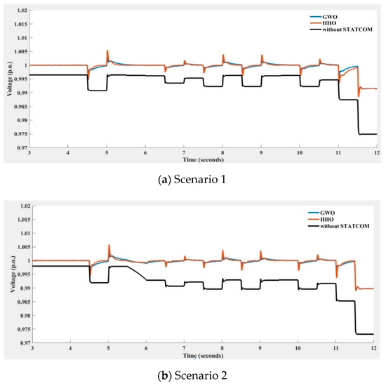

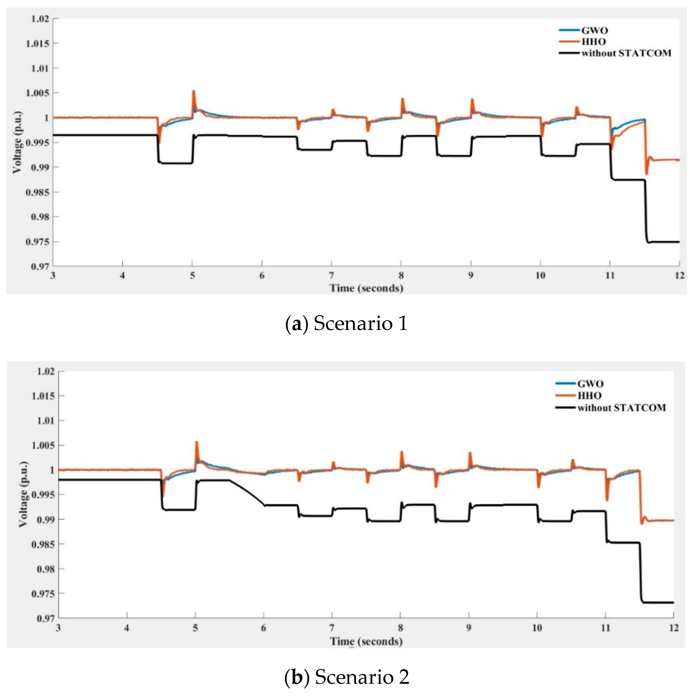
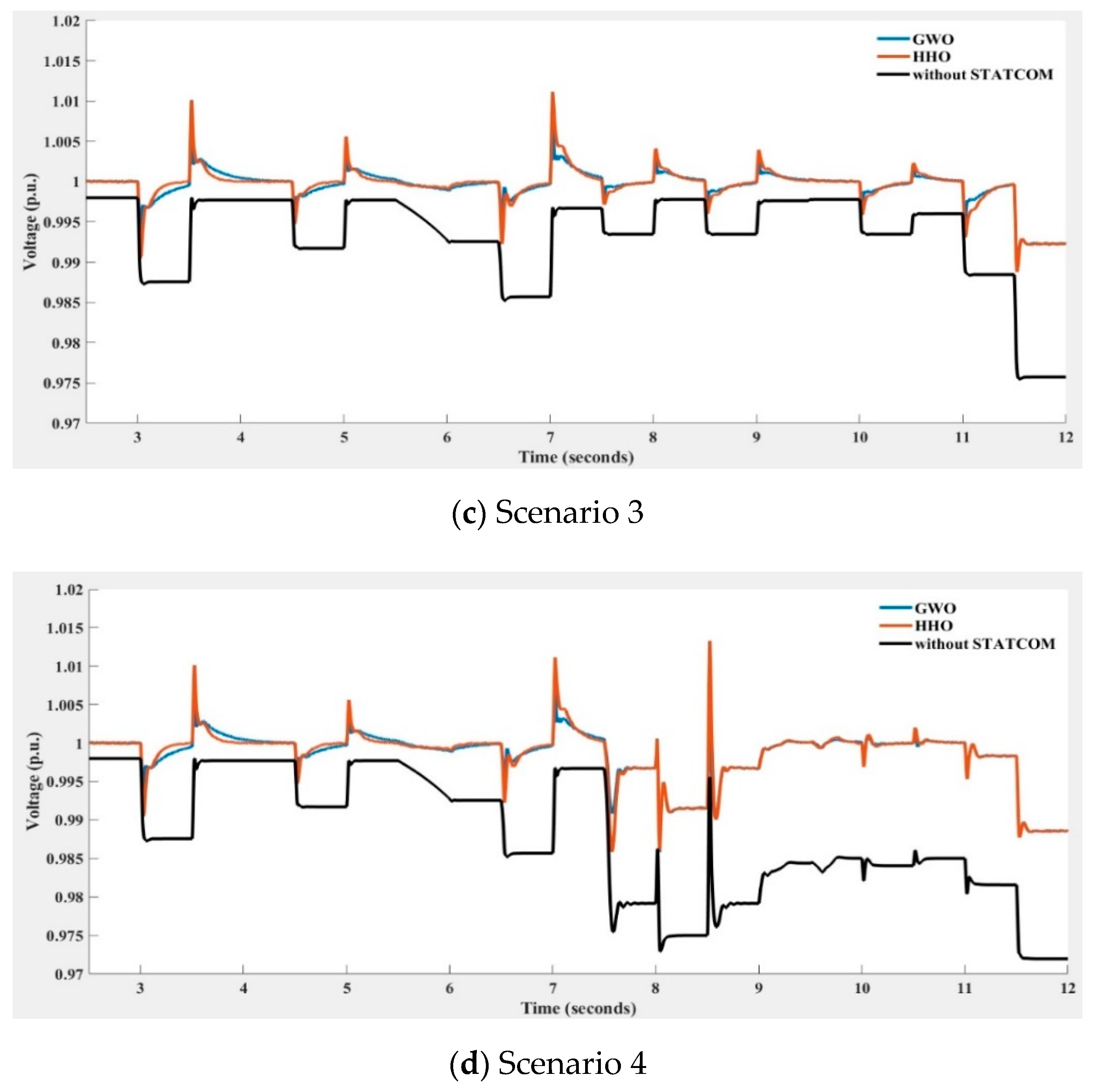
Figure 22.
Voltage at the 33 kV bus with and without STATCOM compensation obtained using GWO (in blue line), HHO (in orange line), and without STATCOM (in black line) for voltage regulator under four various wind turbine power output scenarios (Scenarios 1~4 indicate different degrees of the wind farm output power variation).
In Figure 21, the STATCOM terminal bus voltage depicted with the blue line was obtained with the swarm-based PI controller being implemented in the voltage regulator and the classic PI controller being implemented in the current regulator; the voltage in the red line was obtained when swarm-based PI controllers were implemented at both voltage and current regulators. The black line indicates the voltage without STATCOM compensation. Table 3 lists the mean average percentage errors (MAPEs) of the compensated voltage and the reference (1 p.u.) shown in Figure 20 over ten runs of the compared algorithms. The MAPE is defined in (45).
where NS is the number of total time steps, vn and vref are the compensated and reference voltages at the n-th sampled point, respectively.
Table 3.
MAPEs obtained by the four swarm-based algorithms over ten runs for Figure 20.
By observing Figure 21 and Table 3, it can be seen that the compensation performance of HHO is better than that of the other three algorithms, with GWO ranking second best. It was also found that the STATCOM voltage regulator implemented with the compared swarm-based algorithms alone performed better than those obtained when implementing swarm-based algorithms in both voltage and current regulators.
Figure 22 depicts the STATCOM terminal voltage trends with and without compensation under four scenarios of more drastic wind speed changes leading to stronger WT power output variations when only the voltage regulator is implemented with the HHO and GWO algorithms. The MAPEs of Figure 22 are listed in Table 4. The results of PSO and KH algorithms are not shown because of poor compensation performance compared to HHO and GWO. By observing Figure 22 and Table 4, the implementation of the HHO algorithm in the PI controller of STATCOM voltage regulator yields better compensation performance than that of GWO.
Table 4.
MAPEs obtained by GWO and the HHO algorithms over ten runs of Figure 22.
6. Discussion
In this study, we intended to control the 33 kV bus voltage to as close to the reference voltage (i.e., 1 p.u.) as possible using a STATCOM voltage regulator while implementing the HHO algorithm to compensate the voltage fluctuation associated variations wind farm power output, and to show its superiority over the compared methods. On the basis of the two study cases reported, the following observations are made.
- (1)
- The HHO-based PI controller implemented in the STATCOM voltage regulator provides more effective voltage regulation capability than the PSO, GWO, and KH algorithms, as shown in the results of Figure 21 and Table 3. The mean average error (MAPE) obtained by HHO between the compensated and reference voltages is the lowest among the four algorithms under comparison.
- (2)
- The HHO algorithm outperforms the other three algorithms for STATCOM terminal voltage regulation under different degrees of wind power output variation, as shown in Figure 22 and Table 4. The MAPE increases as the wind farm power output is more drastically changed due to the dynamic responses of STATCOM.
- (3)
- As shown in Figure 21 and Table 3, implementing the HHO algorithm for both STATCOM voltage and current regulators may not yield better compensation performance than implementing the HHO algorithm for the voltage regulator alone. The MAPE of the former is 0.1407, while that of the later is 0.1217. Both voltage and current regulators during STATCOM compensation require a well-coordinated mechanism when the swarm intelligence-based optimization algorithms are implemented in the PI controllers to achieve better performance.
In summary, the HHO algorithm shows satisfactory compensation performance for the STATCOM terminal voltage regulation during variations in offshore wind farm output.
7. Conclusions
This paper presented the Harris Hawk Optimization algorithm implemented in the PI controller of the STATCOM voltage regulator for mitigating the fluctuations in voltage associated with variations in output power of an offshore wind farm with 21 wind turbines. The proposed method was tested under several wind farm output power scenarios to show the usefulness of the proposed solution algorithm. Test results prove that the proposed HHO is superior to the other three compared algorithms in STATCOM terminal voltage regulation.
Although the proposed HHO algorithm offers better compensation performance than PSO, GWO, and KH algorithms, some limitations of the HHO algorithm applied to STATCOM control were observed, and could be improved in the future study, as listed below.
- (1)
- The low population diversity with the single-search method of the HHO algorithm in its exploration stage weakened the global search capability and thus population diversity needs to be improved in order to avoid being trapped in local minima or premature convergence.
- (2)
- An algorithm for the improvement of PI controller gain adjustment is required for the compensation of drastic STATCOM terminal voltage fluctuations.
- (3)
- It is necessary to enhance the coordination between different STATCOM regulators to achieve better compensation in real time.
Overall, the HHO-based PI controller is a promising solution for grid voltage regulation when using STATCOM for renewable energy applications. Future work will focus on applying the HHO algorithm for optimization problems with more variables and constraints, such as microgrid controller design and distributed generation control and planning. The modification or improvement of the HHO algorithm for the STATCOM control will also be a future topic of follow-up research work.
Author Contributions
Conceptualization, G.W.C. and Y.-J.L.; methodology, P.-K.W., J.-T.L. and Z.-W.W.; software, P.-K.W., J.-T.L. and Z.-W.W.; validation, P.-K.W., H.-C.C. and B.-X.H.; investigation, P.-K.W., J.-T.L. and Z.-W.W.; writing—review and editing, G.W.C., Y.-J.L. and P.-K.W., supervision, G.W.C. and Y.-J.L. All authors have read and agreed to the published version of the manuscript.
Funding
This research was funded in part by Ministry of Science and Technology, Taiwan, R.O.C., grant number MOST 110-2221-E-194-028-MY2.
Institutional Review Board Statement
Not applicable.
Informed Consent Statement
Not applicable.
Data Availability Statement
Not applicable.
Conflicts of Interest
The authors declare no conflict of interest.
References
- Rao, P.; Crow, M.L.; Yang, Z. STATCOM control for power system voltage control applications. IEEE Trans. Power Del. 2000, 15, 1311–1317. [Google Scholar] [CrossRef] [Green Version]
- Joshi, J.K.; Behal, A.; Mohan, N. Voltage regulation with STATCOMs: Modeling, control and results. IEEE Trans. Power Del. 2006, 21, 726–735. [Google Scholar]
- Li, K.; Liu, J.; Wang, Z.; Wei, B. Strategies and operating point optimization of STATCOM control for voltage unbalance mitigation in three-phase three-wire systems. IEEE Trans. Power Del. 2007, 22, 413–422. [Google Scholar] [CrossRef]
- Varma, R.K.; Maleki, H. PV solar system control as STATCOM (PV-STATCOM) for power oscillation damping. IEEE Trans. Sustain. Energy 2019, 10, 1793–1803. [Google Scholar] [CrossRef]
- Qi, J.; Zhao, W.; Bian, X. Comparative study of SVC and STATCOM reactive power compensation for prosumer microgrids with DFIG-based wind farm integration. IEEE Access 2020, 8, 209878–209885. [Google Scholar] [CrossRef]
- Merritt, N.R.; Chakraborty, C.; Bajpai, P. An E-STATCOM based solution for smoothing photovoltaic and wind power fluctuations in a microgrid under unbalanced conditions. IEEE Trans. Power Syst. 2022, 37, 1482–1492. [Google Scholar] [CrossRef]
- Zhou, X.; Zhong, W.; Ma, Y.; Guo, K.; Yin, J.; Wei, C. Control strategy research of D-STATCOM using active disturbance rejection control based on total disturbance error compensation. IEEE Access 2021, 9, 50138–50150. [Google Scholar] [CrossRef]
- Varma, R.K.; Khadkikar, V.; Seethapathy, R. Nighttime application of PV solar farm as STATCOM to regulate grid voltage. IEEE Trans. Energy Convers. 2009, 24, 983–985. [Google Scholar] [CrossRef]
- Varma, R.K.; Siavashi, E.; Mohan, S.; McMichael-Dennis, J. Grid support benefits of solar PV systems as STATCOM (PV-STATCOM) through converter control: Grid integration challenges of solar PV power systems. IEEE Electrif. Mag. 2021, 9, 50–61. [Google Scholar] [CrossRef]
- Gu, F.C.; Chen, H.C. An anti-fluctuation compensator design and its control strategy for wind farm system. Energies 2021, 14, 6413. [Google Scholar] [CrossRef]
- Kumar, V.; Pandey, A.S.; Sinha, S.K. Stability improvement of DFIG-based wind farm integrated power system using ANFIS controlled STATCOM. Energies 2020, 13, 4707. [Google Scholar] [CrossRef]
- Xu, Y.; Li, F. Adaptive control of STATCOM for voltage regulation. IEEE Trans. Power Del. 2014, 29, 1002–1011. [Google Scholar] [CrossRef]
- Hong, Y.Y.; Hsieh, Y.L. Interval type-II fuzzy rule-based STATCOM for voltage regulation in the power system. Energies 2015, 8, 8908–8923. [Google Scholar] [CrossRef] [Green Version]
- Ibrahim, A.M.; Gawish, S.A.; El-Amary, N.H.; Sharaf, S.M. STATCOM controller design and experimental investigation for wind generation system. IEEE Access 2019, 7, 50433–150461. [Google Scholar] [CrossRef]
- Valério, D.; da Costa, J.S. Tuning of fractional PID controllers with Ziegler–Nichols-type rules. Signal Process 2006, 86, 2771–2784. [Google Scholar] [CrossRef]
- Liu, C.H.; Hsu, Y.Y. Design of a self-tuning PI controller for a STATCOM using particle swarm optimization. IEEE Trans. Ind. Electron. 2010, 57, 702–715. [Google Scholar]
- Tuzikova, V.; Tlusty, J.; Muller, Z. A novel power losses reduction method based on a particle swarm optimization algorithm using STATCOM. Energies 2018, 11, 2851. [Google Scholar] [CrossRef] [Green Version]
- Hung, Y.H.; Chen, Y.W.; Chuang, C.H.; Hsu, Y.Y. PSO self-tuning power controllers for low voltage improvements of an offshore wind farm in Taiwan. Energies 2021, 14, 6670. [Google Scholar] [CrossRef]
- Qais, M.H.; Hasanien, H.M.; Alghuwainem, S. A grey wolf optimizer for optimum parameters of multiple PI controllers of a grid-connected PMSG driven by variable speed wind turbine. IEEE Access 2018, 6, 44120–44128. [Google Scholar] [CrossRef]
- Yaghoobi, S.; Mojallali, H. Tuning of a PID controller using improved chaotic Krill Herd algorithm. Optik 2016, 127, 4803–4807. [Google Scholar] [CrossRef]
- Kamel, O.M.; Diab, A.A.Z.; Do, T.D.; Mossa, M.A. A novel hybrid ant colony-particle swarm optimization techniques based tuning STATCOM for grid code compliance. IEEE Access 2020, 8, 41566–41587. [Google Scholar] [CrossRef]
- Mosaad, M.I.; Ramadan, H.S.M.; Ajohani, M.; El-Naggar, M.F.; Ghoneim, S.S.M. Near-optimal PI controllers of STATCOM for efficient hybrid renewable power system. IEEE Access 2021, 9, 34119–34130. [Google Scholar] [CrossRef]
- Elkady, Z.; Abdel-Rahim, N.; Mansour, A.A.; Bendary, F.M. Enhanced DVR control system based on the Harris hawks optimization algorithm. IEEE Access 2020, 8, 177721–177733. [Google Scholar] [CrossRef]
- Diab, A.A.Z.; Ebraheem, T.; Aljendy, R.; Sultan, H.M.; Ali, Z.M. Optimal design and control of MMC STATCOM for improving power quality indicators. Appl. Sci. 2020, 10, 2490. [Google Scholar] [CrossRef] [Green Version]
- Abdelsalam, M.; Diab, H.Y.; El-Bary, A.A. A metaheuristic Harris hawk optimization approach for coordinated control of energy management in distributed generation based Microgrids. Appl. Sci. 2021, 11, 4085. [Google Scholar] [CrossRef]
- Heidari, A.A.; Mirjalili, S.; Faris, H.; Aljarah, I.; Mafarja, M.; Chen, H. Harris hawks optimization: Algorithm and applications. Futur. Gener. Comput. Syst. 2019, 97, 849–872. [Google Scholar] [CrossRef]
- MathWorks. Simscape Electrical User’s Guide (Specialized Power Systems), R2019b; MathWorks: Portola Valley, CA, USA, 2019. [Google Scholar]
- Kennedy, J.; Eberhart, R. Particle swarm optimization. Proc. IEEE Int. Conf. Neural Netw. 1995, IV, 1942–1948. [Google Scholar]
- Mirjalili, S.; Mirjalili, S.M.; Lewis, A. Grey wolf optimizer. Adv. Eng. Softw. 2014, 69, 46–61. [Google Scholar] [CrossRef] [Green Version]
- Gandomi, A.H.; Alavi, A.H. Krill herd: A new bio-inspired optimization algorithm. Commun. Nonlinear Sci. Numer. Simul. 2012, 17, 4831–4845. [Google Scholar] [CrossRef]
- Tsili, M.; Papathanassiou, S. A review of grid code technical requirements for wind farms. IET Renew. Power Gener. 2009, 3, 308–332. [Google Scholar] [CrossRef]


Publisher’s Note: MDPI stays neutral with regard to jurisdictional claims in published maps and institutional affiliations. |
© 2022 by the authors. Licensee MDPI, Basel, Switzerland. This article is an open access article distributed under the terms and conditions of the Creative Commons Attribution (CC BY) license (https://creativecommons.org/licenses/by/4.0/).