Transferability of a Battery Cell End-of-Life Prediction Model Using Survival Analysis

Abstract

Electric vehicles are increasingly becoming the vehicle of choice in today’s environmentally conscious society, and the heart of an electric vehicle is its battery. Today, lithium-ion batteries are mainly used to power electric vehicles for its increased energy storage density and longevity. However, in order to estimate battery life, long and costly battery testing is required. Therefore, there is a need to investigate efficient ways that could reduce the amount of testing required by reusing existing knowledge of aging patterns from different kinds of battery chemistry. This work aims to answer two research questions. The first addresses the challenge of battery cell testing data that contain battery cells that do not reach the End-of-Life (EOL) threshold by the time the testing has been completed. For this challenge, we propose to implement survival analysis that is able to handle incomplete data or what is referred to as censored data. The second addresses how to reuse a model trained on one type of battery cell chemistry to predict the EOL of another battery cell chemistry by implementing transfer learning. We develop a workflow to implement a prediction model for one type of battery cell chemistry and to reuse this pre-trained model to predict the EOL for another type of battery cell chemistry.

1. Introduction

The adoption of electric vehicles (EV) is expected to be on an upward trend as demand is getting stronger for clean energy and environmentally friendly alternatives. The EV30@30 Campaign launched in 2017 established a goal to achieve a 30% market share for electric vehicles out of the total vehicles (except two-wheelers) by 2030. This is also in line with the Paris Agreement to reduce carbon emission by at least 40% by 2030 compared to 1990 [1].

Since the battery is the heart of an electric vehicle, it is critical to determine the robustness of the battery through understanding its aging process. As of now, battery manufacturers can only provide a battery lifetime warranty of between eight to ten years before a battery needs to be replaced, which is much shorter than the life of the car itself. Currently, the United States Council for Automotive Research (USCAR) has set an ambitious goal for EV manufacturers to provide a 15-year warranty on battery life by 2020 as the lifetime of cars are also expected to extend for more years. A battery’s end-of-life (EOL) threshold is usually set at between 70% and 80% remaining capacity. Beyond this threshold, the battery capacity degrades rapidly, which also defines the point at which the battery needs to be replaced.

The first challenge in determining warranty periods for batteries is obtaining battery life data from lab experiments that are usually conducted for a period between six months to two years (https://www.mpoweruk.com/testing.htm, accessed on 13 January 2022). This testing process is costly and often needs to be repeated to observe battery cell aging using different kinds of cell chemistry and charging conditions.

The second challenge is that the EOL data points are scarce as battery life degrades linearly and the remaining capacity is still above the EOL threshold at the end of the specified testing period. Extrapolation methods can be used to determine battery life, but it is difficult to validate the models they output without EOL data for the specific battery. Such data are not easy to obtain, thus motivating the study of transfer learning for this purpose.

To address these two challenges, we formulate and study following research questions:

• RQ1: How can survival models be used to predict battery EOL?
• RQ2: How can we transfer a model learned for one type battery cell chemistry to predict the EOL for another type of battery cell chemistry?

2. Background

2.1. Battery EOL Prediction Models

To address the first research question, we investigate existing battery EOL prediction models. Battery EOL prediction is an active research area with many relevant studies using machine learning approaches emerging in recent years. With intelligent techniques [2,3,4], Refs. [5,6] used simpler algorithms that achieved better accuracy levels compared to adaptive filter techniques but are lacking in analyzing uncertainty of the measurement results [7]. Generally, these algorithms also require more training samples to improve accuracy.

Adaptive filtering models [8,9,10] improved the accuracy of battery health prognostics. However, they are highly influenced by the variability in current and temperatures. In [11], Ng et al. used a Naive Bayes (NB) model and showed that it achieves comparable results to Support Vector Machine (SVM). However, they also mentioned that NB loses on accuracy at the critical point when the capacity of the battery reaches the specified threshold; SVM has better predictive power at this phase.

The Gaussian Process Mixture (GPM) approach in [12] compared its performance with Gaussian Process Regression (GPR) and SVM, where the GPM method produced better prediction accuracies. The accuracy metric used is by comparing between the actual number of charge discharge cycles and the predicted number of charge discharge cycles until the battery reaches the EOL threshold. GPM achieved less than one cycle of error while GPR and SVM obtained more than three cycles of error. However, the prediction accuracy of GPM also depends on the amount of training data available to improve its performance.

With the widespread use of neural network approaches in recent years, Zhang et al. [2] used the Recurrent Neural Network (RNN) approach, where results were compared against a simple recurrent neural network (SimRNN), particle filter (PF) and SVM approach. Generally, the long short-term memory recurrent neural network (LSTM-RNN) approach provided better prediction results but still suffers from longer computational time. In [13], the authors applied transfer learning using neural network, but the model still required a lot of training data and known EOL points, which is sometimes a challenge to obtain especially in testing environments.

Common among these studies is the availability of cell data reaching EOL. Usually, this is not the case in practice though. The datasets used were obtained from internal testing experiments. The number of cells used to build and test the prediction models were also small. This is important as battery aging characteristics could differ from one battery to another; therefore, using more battery cells would give better generalization of the expected battery lifespan.

A closely related work by Severson et al. [14] aimed to predict battery cell EOL at an earlier stage by just using the battery cell charge discharge cycle data from the first 100 cycles. The features are based on the log variance of the discharge voltage curve that has a high correlation with the battery cycle life. The authors used an Elastic Net regression method to select the relevant features which combine the strengths of the lasso and ridge regression methods. They developed three models that show increasing prediction accuracy as more features were used, but these features were mainly derived from the discharge voltage curve. The results of this study showed that using data generated from cell testing without any prior knowledge of the aging and degradation mechanisms can be used to predict battery EOL. However, it did not consider other aging factors that can occur in real life battery usage. This information is especially useful for determining battery warranty periods by battery manufacturers and for engineers to optimize battery design for longer lifetimes.

Survival analysis has been used for battery lifetime prediction in the past. For example, Voronov et al. used heavy fleet data for a specific type of cell chemistry [15], while Zhang et al. combined survival analysis with neural networks [16]. Here, we use survival analysis for RQ1, while making sure that the models are transparent enough for transfer, as demanded by RQ2.

For the purpose of model verification and validation, several methods can be considered. Based on the state-of-the-art approaches in reliability engineering, the AVL Load Matrix^TM methodology [17], for example, provides a systematic approach for the definition, optimization and monitoring of the reliability targets in the product development life cycle. This process is designed to ensure high accelerated validation of components as well as target oriented design. Furthermore, it provides a predictive lifetime solution for durability/reliability-relevant components using a physics of failure-based damage model approach. The key elements being the trade-off between the in-field customer usage profile, the optimized and balanced test program and the demonstration of the reliability/durability coverage.

For data-driven models, several recent works included model validation and verification techniques [18,19]. In [18], Weihan et al. employed a processor-in-the-loop approach and combined nominal and noisy data to validate model robustness. In [19], the authors implemented a validation and verification framework using Monte-Carlo simulation and K-L divergence to ensure the accuracy of the prediction models developed.

2.2. Basics of Transfer Learning

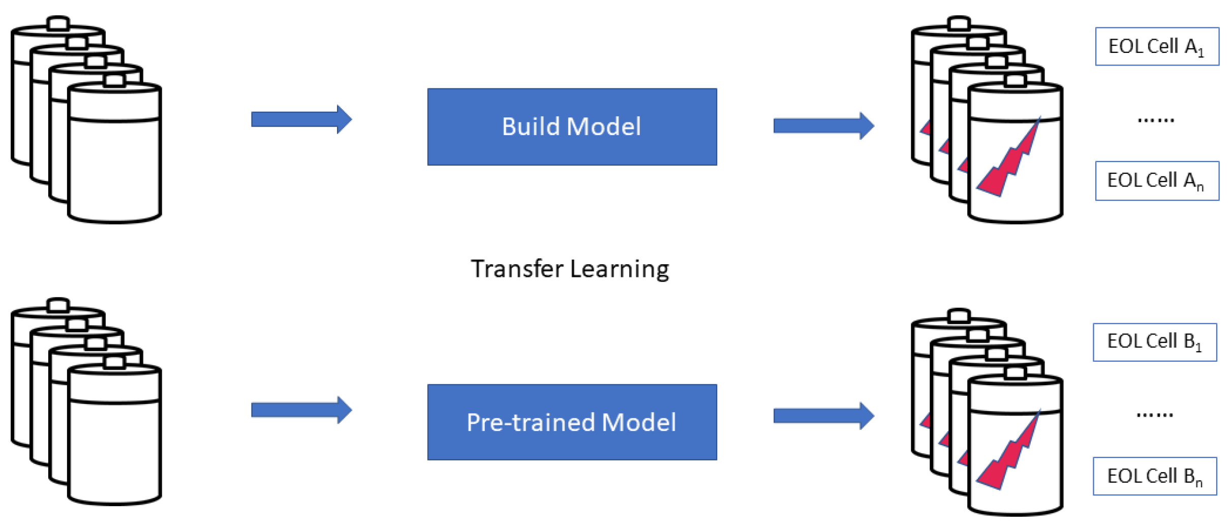
RQ2 refers to the transferability of prediction models. To do this, we investigate the use of transfer learning as an approach to facilitate the transfer of knowledge from the source domain to a target domain. The target dataset usually consists of a much smaller data sample (compared to the source dataset).

Transfer learning involves determining when, what and how knowledge should be transferred from a source domain to a target domain [20]. In this paper, the authors discussed the fundamental questions of what to transfer? and how to transfer?. The question on when to transfer? can be addressed upon evaluating the prediction performance of the target model. If the predictions for the target dataset becomes worse by using a transfer model compared to using the model trained on the target dataset, then we can conclude that using a transfer learning approach may not be the best approach. This is because it can lead to a situation referred to as negative transfer. To answer the question on what to transfer?, we perform an initial analysis on the source and target dataset. We would either have the same set of features or overlapping features in the source and target datasets.

There are three main ways for a model to be transferred from the source domain to the target domain as described in [20]. The instance based method aims to leverage overlapping features between the source and target dataset where a part of the source dataset is assumed to be reusable for learning the target dataset. The instance transfer can be performed using two major techniques, which are the instance re-weighting and importance sampling [20].

The feature based method considers projecting features to provide a common representation for the model transfer. The first step using this method is to identify by learning a set of ideal or good features from the source domain. The definition of good or ideal features depends on the domain experts. This set of features are then transferred to the target domain by means of encoding the learned feature representation [20].

The two approaches above need information at the data level, and because of this, it requires domain knowledge. The third approach, i.e., the model parameter-based method, rather concentrates at the parameter level. At the model level, the main assumption is that the source and target tasks have model hyper-parameter values that follow a common distribution shape. Therefore, the transfer of knowledge is performed by re-using the hyper-parameter values of the source model into the target model [20].

3. Materials and Methods

3.1. Problem Specification

As mentioned, battery cell testing often occurs within a limited time period of between six months and two years. By the end of the testing period, many battery cells do not reach the EOL threshold or are removed from the study if a defect occurs during the testing period. This leads to scarcity in true EOL time points and requires implementing extrapolation methods that are difficult to be validated. Figure 1 depicts the conceptual workflow for addressing RQ1 and RQ2 and is explained hereafter.

Addressing RQ1: We explore the use of survival analysis by considering data points that have not manifested the intended event as censored data. It is based on the assumption that at some point in the study (for drop outs) or after the study is completed, there is still the possibility that the intended event will occur for these cells but the time of event is unknown. Therefore, a binary labeling method is used to mark if a cell has reached its EOL during the study or not. This type of censoring is called right censoring. There are other types of censoring called left censoring and interval censoring, but these are not applicable for this use case.

Addressing RQ2: We explore transfer learning to transfer knowledge already gained from the degradation patterns of one type of battery cell chemistry to predict the EOL for a different type of battery cell chemistry, as described in Figure 2.

To the best of our knowledge, there are no existing techniques that consider applying survival analysis and transfer learning to address incomplete data points and transferring knowledge for battery EOL predictions.

3.2. Collect and Process Battery Life Dataset

As a first step in the framework, we obtain datasets that include battery life testing for two battery cell chemistries, namely the NMC and NCA cell chemistry type from AVL List GmbH. Using a design of experiment (DoE) task, a statistical foundation is formed to determine the life testing configurations. A range is determined for each aging influence parameter that defines the load point configuration to be used when each battery cell is tested in the lab. Each configuration is repeated at least three times.

The characteristics of the datasets used is as shown in

Table 1. Dataset A and dataset B description.

Dataset	Battery Type	Chemistry Type	No of Cells	Duration (in Days)	No of Cells Reaching EOL	No of Censored Cells
Dataset A (source dataset)	18650	NMC	122	840	37	85
Dataset B (target dataset)	18650	NCA	100	525	38	62

. The load point configurations that are used for the experiments are as shown in

Table 2. Load point configurations for dataset A.

Factor	Unit	Min	Max	Factor Levels
Temperature (Temp)	${}^{\circ }$C	−10	40	−10	5	20	40
Charge Current (CC)	A	0.2	2.4	0.2	0.8	2.4
Average Discharge Current (ADC)	A	0	8	0	0.2	1	4	8
Peak Discharge Current (PDC)	A	0.2	14	0.2	3	8	10	14
Frequency (Freq)	Hz	3.33 $\times {10}^{-4}$	0.5	3.33 $\times {10}^{-4}$	0.03	0.1	0.5
State of Charge (SoC)	%	15	95	15	25	55	85	95
Delta State of Charge (DSoC)	%	0.01	80	0.01	2.5	15	50	80

and

Table 3. Load point configurations for dataset B.

Factor	Unit	Min	Max	Factor Levels
Temperature (Temp)	${}^{\circ }$C	0	45	0	20	30	45
Charge Current (CC)	A	0	0.5	0	0.05	0.5
Average Discharge Current (ADC)	A	0	2	0	0.2	0.3	0.75	0.9	1	1.5	2
Peak Discharge Current (PDC)	A	0	3	0.2	1.5	3
Frequency (Freq)	Hz	0	0.5	0	3.0 $\times {10}^{-4}$	3.33 $\times {10}^{-4}$	0.2	0.25	0.5
State of Charge (SoC)	%	15	95	15	25	40	55	70	85	95
Delta State of Charge (DSoC)	%	0	80	0	2.5	20	30	50	80

. The factor levels column show the values for which each configuration was tested.

The data collected show the capacity degradation of each battery cell over time. The data preprocessing step involves taking the final capacity measurement over the nominal capacity to determine the remaining capacity left in the battery cell.

If the remaining capacity percentage is at 80% or less, the battery cell is considered to have reached EOL and the status is labeled as ‘1’; otherwise, the cell is still active and is labeled as ‘0’ to indicate that the cell has not reached EOL, or what is called a censored cell.

3.3. Characterizing the Battery Aging Trend

The next step after data processing is to analyse the aging patterns of the source and target dataset. This step is critical to form an initial impression on the degradation patterns of the two battery cell chemistries.

To characterize the battery aging trend, we use non-parametric survival models. Using this approach gives a visual understanding on how the battery cells were aging over time and their survival patterns. We also use line charts and the log-rank model to statistically evaluate whether there are any similarities between the aging trend in source dataset A compared to the target dataset B.

3.4. RQ1: Developing a Battery EOL Prediction Model

To select a suitable model, we first explore both semi-parametric and parametric survival models that could fit the goal of this use case. We develop the Cox-PH model that shows the influences of each feature on the aging of battery cells over time. For example, we are able to observe the influence of each temperature setting on the survival rate of the battery cells. The Cox-PH model is also generally used to determine hazard ratios between different groups of factors. However, the model is not suitable for the purpose of time to event predictions. Using semi-parametric models does not require the knowledge of the distribution. Since the goal of this study is to predict battery cell EOL, we had to consider other methods.

With further research, we find that EOL predictions to be common in reliability analysis with applications in engineering and manufacturing [21]. Accelerated Failure Time (AFT) models are more suitable where time to event prediction models can be developed. This fell into the parametric survival analysis approach. As it is a parametric-based model, we use descriptive and visual approaches to determine which distribution type would best fit the data.

3.4.1. Model Selection

For the purpose of predicting battery cell EOL, we select the Accelerated Failure Time (AFT) parametric survival model. AFT models can model the effects of covariates on survival time. It assumes that the effect of the covariate can either accelerate or decelerate survival time and is useful when modeling EOL of mechanical components, which results from an underlying mechanical process that affects the performance over time.

In reliability or lifetime data analysis, the common parametric distributions that are applied are the exponential, Weibull, log-normal and log-logistic distributions [21]. As we are interested in predicting time to event, the AFT model is chosen, since it defines the relationship of the survival function for every time $t\in T$, $S\left(t\right|X)$ and the covariates. The equation below is cited and summarized from [22]:

$$S\left(t\right|X)=S_o[texp\left({\beta }^{t}X\right)]$$

(1)

where

t	= survival times;
X	= column vector of covariates $X_1,X_2,\dots ,X_p$;
$S_o$	= baseline survival function;
${\beta }^t$	= vector of regression coefficients (${\beta }_1$,${\beta }_2$, …, ${\beta }_p$).

The factor $exp\left({\beta }^{t}X\right)$ is the accelerator factor which accelerates the survival function with covariate $X=0$. The AFT model assumes that at every time point t the effects of the covariates remains the same but is multiplied by the accelerator factor $exp\left({\beta }^{t}X\right)$.

The covariates and the survival times can also be described using a linear equation between the logarithm of survival time and the covariate X as follows:

$$Y=log\left(T\right)=\mu +{\theta }^{t}X+\sigma W$$

(2)

where $\mu$ is the slope, $\sigma >0$ is an unknown scale parameter, ${\theta }^t=({\theta }^1,{\theta }^2,\dots ,{\theta }^p$) is a vector of regression coefficients, $\theta =-\beta$, $\sigma$ is a scale parameter and W is a distribution error that is a random variable and depicts a certain parametric distribution. A related parametric for T exist for every distribution W.

When using parametric models, assumptions are made on the distribution of the survival time where a predictable pattern can be observed. An advantage of using a parametric method is its ability to predict the time to event for periods after an event has occurred that is often used when we need to predict failure time. Here, based on domain practices [23], we use the Weibull distribution or what is often called as AFT Weibull as the chosen prediction model.

$$S\left(t\right)=exp[-{\left(\lambda t\right)}^p]$$

(3)

In Equation (3), two parameters describe the Weibull distribution which are the scale parameter, $\mathit{\lambda }$, and the shape parameter, p. The shape of the probability density function can take on a variety of forms based on the value of p. If shape, p < 1, this results in a monotonically decreasing instantaneous hazard, $h\left(t\right)$ (see details in Equation (4)) with time, p = 1 yields a constant hazard with time (exponential) and p > 1 reflects an instantaneous hazard that increases with time. To check if the data follow the Weibull distribution, we used a visual analysis that showed the log cumulative hazard as a function of log time.

$$h\left(t\right)=\underset{\delta t\to 0}{lim}\frac{Pr(t\le T<t+\delta t\mid T\ge t)}{\delta t}$$

(4)

For the feature selection step, we use statistical approaches, namely backward selection, forward selection [24] and the Bayesian Information Criterion (BIC) [25]. The next step is to to train these models based on different distribution types and compare the prediction results, which is discussed in the next section.

3.4.2. Model Evaluation Criteria

The evaluation criteria that are used to compare the performance of the prediction models are based on calculating the root mean squared error (RMSE). The RMSE shows the standard deviation of the prediction errors between the actual EOL and the predicted EOL in days; while the prediction errors depicts the difference between the prediction value and the actual, the RMSE shows the spread of these prediction errors, also called the residuals.

3.5. RQ2: Investigating the Transferability of Battery EOL Prediction Models

In this step, we implement a transfer learning approach that can reuse the prediction model built on the source dataset A to predict the EOL of battery cells in the target dataset B of a different cell chemistry type. Therefore, the next goal is to determine what part of source model A can be transferred for target model B and how. For this purpose, we investigate several transfer learning strategies. However, due to time constraints, we implement one of the transfer learning approaches, i.e., the model parameter-based approach. We then develop five model configurations by either transferring both the coefficients and intercept or separately from the source model to the target model.

We also develop a new approach where we implement a weighting mechanism that combines the weighted parameters from both source dataset A and target dataset B. We achieve this by using the weights calculated for dataset A and dataset B and multiplying the weights with the covariance and coefficients of both datasets, as shown in

Table 4. Model design configurations.

Configuration	Description
1	Build the prediction model by using the target dataset B. This configuration acts as the baseline model to evaluate model performance improvement. Split training and validation data using a 70:30 ratio. This split ratio is selected based on the dataset size and to ensure there are sufficient data for training and validation. Iterate split over 500 loops to randomize the dataset.
2	Train source dataset A and train 70% of target dataset B. Transfer coefficients (model parameters) only from source model A to target model B. Validate on 30% of the dataset B target model.
3	Train source dataset A and train 70% of target dataset B. Transfer intercept only from source model A to target model B. Validate on 30% of target dataset B.
4	Train source dataset A and train 70% of target dataset B. Transfer both model parameters and intercept from source model A to target model B. Validate on 30% of target dataset B
5	Using a weighting approach, weights are determined by getting the weighted mean for source dataset A and target dataset B. $$\begin{array}{ccc}\hfill w_{dat{a}_A}& =& \frac{n_{dat{a}_A}}{n_{dat{a}_A}+n_{dat{a}_B}}\hfill \end{array}$$ (5) $$\begin{array}{ccc}\hfill w_{dat{a}_B}& =& \frac{n_{dat{a}_B}}{n_{dat{a}_A}+n_{dat{a}_B}}\hfill \end{array}$$ (6) Multiply weights with the covariance of the source dataset A and target dataset B models and sum the source dataset A and target dataset B covariance. Assign these new covariance values to the target prediction function for dataset B. $$X_{dat{a}_B}=w_{dat{a}_A}{X}_{dat{a}_A}+w_{dat{a}_B}{X}_{dat{a}_B}$$ (7) Multiply weights with the coefficients of source dataset A and target dataset B models and sum these to become the new coefficients for the target prediction function for dataset B. $${\beta }_{dat{a}_B}=w_{dat{a}_A}{\beta }_{dat{a}_A}+w_{dat{a}_B}{\beta }_{dat{a}_B}$$ (8) Using these new covariance and coefficient weights, we validate on 30% of target dataset B to observe if there will be further improvements to the model. where: n = the number of samples X = covariance matrix $\beta$ = coefficient vector

.

3.5.1. Experiment-Based Model Selection Process

To transfer knowledge from dataset A to dataset B aging prediction, we employ the model parameter-based approach.

Formally, the mapping of the parameters can be written as follows:

$$f\left(x\right)=\langle \theta ,x\rangle ={\theta }^{T}x=\sum _{i=1}^m{\theta }_i{x}_i$$

(9)

Specification of Candidate Models

From this mapping, several models can be derived from making assumptions on the similarities shared between the datasets either with the coefficients or the intercept.

Inspired by the work done in [26] for transfer learning in regression cases, we consider that we may not know the distribution of the target dataset since the idea is to also reduce the requirement for labeled target data. Therefore, the following models are configured as follows:

• Model 1: Assume that the source and target dataset share the same coefficients and the intercept stays the same;
• Model 2: Assume that the source and target dataset share the same intercept but not the model coefficients;
• Model 3: Assume that the source and target dataset share the same coefficients but not the model intercept;
• Model 4: Combine the weighted sum coefficient and weighted sum covariance to form the new coefficient and covariance for the target chemistry prediction model.

In model 4, we propose a weighting approach to test the possibility of leveraging the aging patterns, observed from fewer observations collected from the target dataset, to augment the prediction model for better performance.

Although we may not be expecting enough target data available, the idea is mainly to show whether combined knowledge gained from different types of battery cell chemistries could further improve the generalizability of the model.

Design of Alternative Configurations

In the next section, we apply the AFT survival model using a Weibull distribution trained on dataset A, to investigate if a transfer learning method can be employed to improve the prediction function for dataset B.

We then develop several model configurations, as shown in Table 4.

3.5.2. Criteria for the Comparison of the Configurations

How do we know if the transfer method is actually improving the predictions for the target dataset? To answer this question, we begin with building a prediction model using the target dataset alone. We train and test the model only on dataset B. This model acts as the baseline for which the subsequent configurations using the model parameter-based transfer approaches is compared against. If we observe a reduction in the RMSE, this shows that leveraging the knowledge captured from modeling the aging pattern in dataset A can be used to predict the EOL of a different battery chemistry.

In order to select which model configuration to use, we employ a resampling approach. We train and test using a split ratio of 70:30 on each of these models and on each distribution type with a seed loop of 500. The RMSE metric based on battery cells that have reached EOL is used as the evaluation criteria to select the combination of features that result with the lowest prediction error. The train and test split ratio was selected randomly based on data availability. The reason for not using censored data here is because the estimated values will be beyond the survived days; therefore, it will not give an accurate result.

4. Results and Discussion

Figure 3 provides a recap on the steps taken to build the source and target model. The results of each step are explained in the following sections.

4.1. Characterizing the Battery Aging Trend

From the capacity measurements collected after every reference test procedure, we observe that the capacity degradation is linear in the beginning. Upon reaching 80% available capacity, we notice a rapid decline of available capacity that led to the definition of the battery EOL threshold at 80%. Where abnormalities were detected, we sourced for opinions from domain experts to explain the trend. Preprocessing the battery life dataset was essential to ensure that the raw dataset collected is transformed into the dataset needed when implementing survival models.

Figure 4 show the battery cells from dataset A with a stronger linear aging trend, where some battery cells were experiencing more rapid aging than others. This can be explained through the different life testing configurations for the temperature of the casing and state of charge.

Similarly, dataset B shows more variability in the aging of the different battery cells. There were also many occurrences of the battery cells with capacities increasing and dropping over time. These oscillations could result from temperature conditioning. There is also the possibility of capacity spikes when the battery cell goes into a rest period, where some chemical reaction occurs during battery usage and chemical products accumulate near the electrodes. In this situation, the battery goes into a rest period to melt these chemicals and this eventually could lead to a self-charging scenario.

In general, tracing of experiment influences is not trivial. Our visualization scheme demonstrates the differences between the two datasets, and thus, give an aid to an expert in deciding whether a dataset should be used for transfer learning or not.

4.2. RQ1: Developing the Battery EOL Prediction Model

As mentioned earlier, we employed a visual analysis to determine the distribution type to be used for the AFT survival model, as shown in Figure 5. We compared the theoretical assumption with empirical observations. We observe that the log-normal, log-logistic and Weibull distribution closely fits the source dataset.

As there are a large number of factors that needed to be considered for the model selection, we employed automatic techniques for the feature selection step. We applied a forward selection, backward elimination and exhaustive approach using a probabilistic model, BIC [25], which resulted in several model suggestions, as shown in Figure 6. The BIC selection criteria measure the trade-off between the model fit and complexity of the model. A lower BIC value indicates a better model and gives preferences for simpler models.

This step resulted in several possible models upon which we employ a resampling approach and train and test with a split ratio of 70:30 on each of these models and on each distribution type with a seed loop of 500. This split ratio was selected randomly based on the data availability for both training and testing.

Table 5. Top three out of sample prediction results.

No	Model	Log-Logistic	Log-Normal	Weibull
1	EOL = ${\beta }_0+{\beta }_1\ast ADC2+{\beta }_2\ast Temp:CC+{\beta }_3\ast Temp:PDC+{\beta }_4\ast CC:DSoC+{\beta }_5\ast Temp:SoC$	219.03	226.10	313.72
2	EOL = ${\beta }_0+{\beta }_1\ast ADC2+{\beta }_2\ast Temp:PDC+{\beta }_3\ast CC:DSoC+{\beta }_4\ast Temp:SoC$	243.59	255.72	353.45
3	EOL = ${\beta }_0+{\beta }_1\ast SoC+{\beta }_2\ast Temp2+{\beta }_3\ast ADC2+{\beta }_4\ast SoC2+{\beta }_5\ast Temp:PDC+{\beta }_6\ast CC:PDC+{\beta }_7\ast CC:DSoC+{\beta }_8\ast Temp:SoC+{\beta }_9\ast Freq:SOC$	1453.80	340.12	1.35198 $\times {10}^{18}$

show the top three models with the lowest prediction errors (in number of days). A lower value shows better predictions. Model number 1 with five regressors ($ADC2,Temp:CC,Temp:PDC,CC:DSoC,Temp:SoC$) resulted with the lowest RMSE across all distribution types. Interestingly, several distributions are closely fitting the data, namely the log-normal, log-logistic and Weibull distribution.

Our results confirm that simple regression models are appropriate and adequate for prediction. This agrees with the findings of Meeker and Escobar [21] on the potential methods for statistical analysis, and with the popularity of such methods for failure prediction and reliability analysis [15,16]. Accordingly, we chose Weibull distribution for RQ2.

Figure 7 provides the list of parameters, coefficient values and the scale hyperparameter of the Weibull distribution. As mentioned in Section 3.4.1, the Weibull shape parameters are 1/scale.

4.3. RQ2: Investigate Transferability of Battery EOL Prediction Models

We calculate an average RMSE on EOL events from the 500 iterations and the results of the average RMSE for each model configuration are as shown in

Table 6. Model configuration results.

No	Experiment Type	Training and Testing Data Split 70:30
1	Train on target dataset B and validate on target dataset B	923.2991
2	Transfer source model coefficients only and validate on target dataset B	846.7398
3	Transfer source model intercept only and validate on target dataset B	708.2903
4	Transfer source model coefficients and intercept to target dataset B model	691.4873
5	Use weighted sum coefficient and weighted sum covariance	550.9872

.

The first model configuration is designed to capture situations where only a small validation dataset can be obtained. In the case of dataset B, since the experiment duration was short and had many censored observations, the dataset is not sufficient to make reliable predictions especially for battery cells that have reached EOL.

In the second configuration, we leverage the knowledge gained from training on dataset A by transferring only the model coefficients to the target model. The results indicate a prediction error reduction by 8.3%.

In the third configuration, we test on retaining the target model coefficients and only reuse the intercept from the source model. The results show a further prediction error reduction by 23.3%.

In the fourth configuration, both the source model coefficients and intercept are transferred into the target model. Here, we assume that the two battery chemistries share the same behavior. Interestingly, the target prediction model show reduction in RMSE by about 25%, suggesting that this assumption was valid.

In the fifth configuration, we aim to use the best of both worlds. Here, the knowledge from dataset A and dataset B is leveraged, and surprisingly, the results show further reduction in the RMSE by 40%. This approach seemed to have worked best with the lowest RMSE compared to earlier configurations.

Hence, despite the differences between the two datasets, our configurations have shown that low values of prediction error can be achieved while considering relatively few variables. These findings are a stepping stone for the possibility of requiring only a small amount of target dataset to predict battery cell EOL. However, future work would benefit from further experiments with different configurations of training, validation and testing datasets, and to test on other types of battery cell chemistry to verify these findings.

5. Conclusions

In summary, this study was mostly driven by discovery of new approaches to build a more reliable battery EOL prediction model. We also determined whether transfer of knowledge gained from predicting the EOL of one type of battery cell chemistry can be used for another type of battery cell chemistry. It was encouraging to observe the use of survival models that assisted in a clearer understanding of the survival patterns between different types of battery cell chemistry. This research also provided a way for survival models to be reused by implementing several transfer learning methods.

The above-mentioned process will be useful to validate purely data-driven methods and we suggest the following steps to be considered for future work:

• To seek an opinion from domain experts especially reliability engineers who can assist with validating the results and methods used.
• To acquire testing datasets from other types of battery cell chemistry to improve model robustness and further confirm the tested hypotheses.
• To acquire a larger dataset so that the trained model can be tested on purely unseen data and to allow for different splits of training, validation and testing data.
• To observe data from the field and investigate how the usage profile can influence the battery cell aging.

As this was also a first attempt to use transfer learning on survival models, there is a need for further testing on several different datasets. Nevertheless, this study showed promising results that it is possible to perform transfer learning using survival models that may also be applied to other domains of engineering.

References

1. Agency, I.E. Global EV Outlook 2019; IEA: Paris, France, 2019; p. 141. [Google Scholar]
2. Zhang, Y.; Xiong, R.; He, H.; Pecht, M.G. Long short-term memory recurrent neural network for remaining useful life prediction of lithium-ion batteries. IEEE Trans. Veh. Technol. 2018, 67, 5695–5705. [Google Scholar] [CrossRef]
3. Wang, S.; Zhao, L.; Su, X.; Ma, P. Prognostics of lithium-ion batteries based on battery performance analysis and flexible support vector regression. Energies 2014, 7, 6492–6508. [Google Scholar] [CrossRef] [Green Version]
4. Wang, D.; Miao, Q.; Pecht, M. Prognostics of lithium-ion batteries based on relevance vectors and a conditional three-parameter capacity degradation model. J. Power Sources 2013, 239, 253–264. [Google Scholar] [CrossRef]
5. Long, B.; Xian, W.; Jiang, L.; Liu, Z. An improved autoregressive model by particle swarm optimization for prognostics of lithium-ion batteries. Microelectron. Reliab. 2013, 53, 821–831. [Google Scholar] [CrossRef]
6. Chen, Y.; Miao, Q.; Zheng, B.; Wu, S.; Pecht, M. Quantitative analysis of lithium-ion battery capacity prediction via adaptive bathtub-shaped function. Energies 2013, 6, 3082–3096. [Google Scholar] [CrossRef]
7. Lipu, M.S.; Hannan, M.A.; Hussain, A.; Hoque, M.M.; Ker, P.J.; Saad, M.H.; Ayob, A. A review of state of health and remaining useful life estimation methods for lithium-ion battery in electric vehicles: Challenges and recommendations. J. Clean. Prod. 2018, 205, 115–133. [Google Scholar] [CrossRef]
8. Zheng, X.; Fang, H. An integrated unscented kalman filter and relevance vector regression approach for lithium-ion battery remaining useful life and short-term capacity prediction. Reliab. Eng. Syst. Saf. 2015, 144, 74–82. [Google Scholar] [CrossRef]
9. Miao, Q.; Xie, L.; Cui, H.; Liang, W.; Pecht, M. Remaining useful life prediction of lithium-ion battery with unscented particle filter technique. Microelectron. Reliab. 2013, 53, 805–810. [Google Scholar] [CrossRef]
10. Wang, D.; Yang, F.; Tsui, K.L.; Zhou, Q.; Bae, S.J. Remaining Useful Life Prediction of Lithium-Ion Batteries Based on Spherical Cubature Particle Filter. IEEE Trans. Instrum. Meas. 2016, 65, 1282–1291. [Google Scholar] [CrossRef]
11. Ng, S.S.; Xing, Y.; Tsui, K.L. A naive bayes model for robust remaining useful life prediction of lithium-ion battery. Appl. Energy 2014, 118, 114–123. [Google Scholar] [CrossRef]
12. Li, L.; Wang, P.; Chao, K.H.; Zhou, Y.; Xie, Y. Remaining useful life prediction for lithium-ion batteries based on Gaussian processes mixture. PLoS ONE 2016, 11, e0163004. [Google Scholar] [CrossRef] [PubMed] [Green Version]
13. Zhang, A.; Wang, H.; Li, S.; Cui, Y.; Liu, Z.; Yang, G.; Hu, J. Transfer Learning with Deep Recurrent Neural Networks for Remaining Useful Life Estimation. Appl. Sci. 2018, 8, 2416. [Google Scholar] [CrossRef] [Green Version]
14. Severson, K.A.; Attia, P.M.; Jin, N.; Perkins, N.; Jiang, B.; Yang, Z.; Chen, M.H.; Aykol, M.; Herring, P.K.; Fraggedakis, D.; et al. Data-driven prediction of battery cycle life before capacity degradation. Nat. Energy 2019, 4, 383–391. [Google Scholar] [CrossRef] [Green Version]
15. Voronov, S.; Frisk, E.; Krysander, M. Data-Driven Battery Lifetime Prediction and Confidence Estimation for Heavy-Duty Trucks. IEEE Trans. Reliab. 2018, 67, 623–639. [Google Scholar] [CrossRef] [Green Version]
16. Zhang, J.; Wang, S.; Chen, L.; Guo, G.; Chen, R.; Vanasse, A. Time-Dependent Survival Neural Network for Remaining Useful Life Prediction. In Advances in Knowledge Discovery and Data Mining; Yang, Q., Zhou, Z.H., Gong, Z., Zhang, M.L., Huang, S.J., Eds.; Springer International Publishing: Cham, Switzerland, 2019; pp. 441–452. [Google Scholar]
17. Denkmayr, K. AVL’s reliability engineering process for engine development. In Annual Reliability and Maintainability Symposium; IEEE: Piscataway, NJ, USA, 2003; pp. 455–458. [Google Scholar]
18. Li, W.; Sengupta, N.; Dechent, P.; Howey, D.; Annaswamy, A.; Sauer, D.U. One-shot battery degradation trajectory prediction with deep learning. J. Power Sources 2021, 506, 230024. [Google Scholar] [CrossRef]
19. Zhang, Y.; Xiong, R.; He, H.; Pecht, M. Validation and verification of a hybrid method for remaining useful life prediction of lithium-ion batteries. J. Clean. Prod. 2019, 212, 240–249. [Google Scholar] [CrossRef]
20. Pan, S.J.; Yang, Q. A Survey on Transfer Learning. IEEE Trans. Knowl. Data Eng. 2010, 22, 1345–1359. [Google Scholar] [CrossRef]
21. Meeker, W.Q.; Escobar, L.A. Statistical Methods for Reliability Data; Wiley: New York, NY, USA, 1998. [Google Scholar]
22. Faruk, A. The comparison of proportional hazards and accelerated failure time models in analyzing the first birth interval survival data. J. Phys. Conf. Ser. 2018, 974, 012008. [Google Scholar] [CrossRef] [Green Version]
23. Abernethy, R.B. The New Weibull Handbook, 5th ed.; Robert B. Abemethy: New Cordell, OK, USA, 2018. [Google Scholar]
24. Berk, K.N. Forward and backward stepping in variable selection. J. Stat. Comput. Simul. 1980, 10, 177–185. [Google Scholar] [CrossRef]
25. Schwarz, G. Estimating the dimension of a model. Ann. Statist. 1978, 6, 461–464. [Google Scholar] [CrossRef]
26. Bouveyron, C.; Jacques, J. Adaptive linear models for regression: Improving prediction when population has changed. Pattern Recognit. Lett. 2010, 31, 2237–2247. [Google Scholar] [CrossRef] [Green Version]
Figure 1. Conceptual framework.
Energies 15 02930 g001
Figure 2. Main idea for battery cell aging prediction transferability.
Energies 15 02930 g002
Figure 3. Model development workflow.
Energies 15 02930 g003
Figure 4. Capacity degradation trend over time. (a) Dataset A depicts the capacity degradation trend for NMC cells, while (b) dataset B depicts the capacity degradation trend for NCA cells. Each line represents one battery cell. Cells were tested under different test load conditions (as shown in Table 2 and Table 3) that result in some cells degrading at different rates. The majority of the cells were degrading at a linear trend but did not reach EOL threshold by the end of the testing period.
Energies 15 02930 g004
Figure 5. Distribution analysis for the source dataset. (a) Exponential distribution. (b) Log-logistic distribution. (c) Log-normal distribution. (d) Weibull distribution.
Energies 15 02930 g005
Figure 6. Model selection process. (a) Exhaustive search using BIC. (b) Forward selection using BIC. (c) Backward elimination using BIC.
Energies 15 02930 g006
Figure 7. Weibull AFT model fit.
Energies 15 02930 g007