Mixed-Integer Linear Programming Model to Assess Lithium-Ion Battery Degradation Cost

Abstract

This work proposes a mixed-integer linear programming model for the operational cost function of lithium-ion batteries that should be applied in a microgrid centralized controller. Such a controller aims to supply loads while optimizing the leveled cost of energy, and for that, the cost function of the battery must compete with the cost functions of other energy resources, such as distribution network, dispatchable generators, and renewable sources. In this paper, in order to consider the battery lifetime degradation, the proposed operational cost model is based on the variation in its state of health (SOH). This variation is determined by experimental data that relate the number of charge and discharge cycles to some of the most important factors that degrade the lifespan of lithium-ion batteries, resulting in a simple empirical model that depends on the battery dispatch power and the current state of charge (SOC). As proof-of-concept, hardware-in-the-loop (HIL) simulations of a real microgrid are performed considering a centralized controller with the proposed battery degradation cost function model. The obtained results demonstrate that the proposed cost model properly maintains the charging/discharging rates and the SOC at adequate levels, avoiding accelerating the battery degradation with use. For the different scenarios analyzed, the battery is only dispatched to avoid excess demand charges and to absorb extra power produced by the non-dispatchable resources, while the daily average SOC ranges from 48.86% to 65.87% and the final SOC converges to a value close to 50%, regardless of the initial SOC considered.

1. Introduction

1.1. Background

One of the most significant changes to electrical systems around the world has been the rapid expansion of distributed energy resources (DERs) [1]. DERs are small-scale electricity supply or demand resources that are connected to a local distribution system, which may compose a microgrid system. They can include emergency diesel generators (EDGs), renewable energy sources (RESs), energy storage systems (ESSs), controllable loads, and others [2,3,4]. Microgrids that integrate multiple DERs have become common, increasing the need to properly control their sources and loads in order to ensure an optimized operation [4,5,6,7].

In these systems, EESs can be used to improve system stability and operational safety in both islanded and grid-connected operation conditions. They are also able to absorb excess power generated by RESs, to reduce demand charges by discharging the stored energy during peak demand periods, to avoid the usage of EDGs reducing CO₂ emissions, and other benefits [8,9]. Typical ESSs employed in microgrids are batteries, supercapacitors, flywheels, compressed air, and pumped hydroelectric technologies [10,11]. Among them, lithium-ion (Li-ion) battery ESSs (BESSs) have become one of the most promising solutions for microgrid networks due to their high-energy and high-power densities [12].

1.2. Related Works and Research Gap

Unlike conventional dispatchable generators, which have an operating cost that is related to fuel consumption, the main cost of a BESS is related to its initial investment. However, each charge and discharge cycle degrades the battery lifetime and, depending on how the cycles are performed, the degradation can be worse [13]. Thus, due to the variation in the useful life according to its operation, the degradation of the battery could, in a certain way, be directly associated with a method for estimating the operating cost of a battery [14,15]. Nevertheless, most works published in the technical literature do not explicitly assess the cost of the battery resulting from degradation. Often, the battery operating cost is calculated by normalizing the initial capital cost to the daily cost, assuming constant operating hours and capacity factors [16]. However, this does not reflect the change in cost as battery usage varies throughout the day. In other cases, the battery operating cost is normalized per unit of energy (USD/kWh) to a constant value, such as the levelized cost of energy (LCOE) [17]. Despite taking into account the amount of energy used by the battery, these methods assume a constant operating condition and that the battery life expectancy does not change.

The existing battery life prediction methodologies in the literature can be divided into electrochemical and empirical approaches [18,19]. Electrochemical lifetime prediction uses physical models in conjunction with chemical reaction equations [20]. This type of approach is the most accurate and insightful, as it captures physical and chemical characteristics as part of the model. However, the large number of physical and chemical parameters needed makes the process quite complicated, in addition to requiring information not available from manufacturers, which makes the widespread use of these models unfeasible [18]. By contrast, empirical approaches use experimental curve fitting to find general equations from discrete measurement points, reducing the model complexity [21,22]. While this approach is independent of the type of battery chemistry, the curves and individual factors that degrade lifespan are different for each battery type. In the case of lithium-ion and lead acid batteries, the factors that influence the lifespan are usually the same [23]. Among the most important factors are operating at extreme temperature, high charging and discharging rates, as well as cycling to high and low states of charge (SOCs) [21,22,23,24].

A figure of merit widely used to represent the battery lifetime degradation is the state of health (SOH) [22]. A battery’s SOH represents the current condition of the battery compared to its original factory condition. Depending on how it is defined (there is no standard in the literature), the SOH decreases as the battery is used. When the battery’s SOH reaches a certain level (e.g., 80%), the battery is considered to have reached the end of its useful life and needs to be replaced. In general, battery management systems (BMSs) provide battery health status information, but it may be calculated sporadically and may not have enough resolution to be used in the battery cost calculation, in addition to the lack of a pattern in its estimation [25].

1.3. Contributions

In light of the foregoing considerations, we propose a simple empirical operational cost model for lithium-ion (Li-ion) batteries based on the variation in the state of health in order to consider its degradation in power dispatch problems, but without using the SOH information from the BMS. The proposed cost model is a function of battery dispatch power and current SOC, and it uses the information from experimental data that relate the number of charge/discharge cycles with the most important factors that degrade its lifespan, being applicable to optimal dispatch algorithms for microgrid control based on mixed-integer linear programming (MILP).

The remainder of this study is organized as follows. Section 2 introduces the proposed multi-factor degradation cost model of the battery energy storage system. Section 3 presents the mathematical modeling and the complete cost function to be applied in a microgrid controller system using mixed-integer linear programming, followed by the obtained simulation results using hardware-in-the-loop (HIL) in Section 4. Lastly, Section 5 presents a comparison with other state-of-the-art solutions, and the conclusions are drawn in Section 6.

2. Multi-Factor Battery Degradation Cost Model

The proposed operational cost model for the power dispatch of a BESS is given by:

$$fba{t}_{b,t}(p_{b,t})=c_b·\frac{\mathsf{\Delta }t}{T_n}·f_{\mathsf{\Delta }SOH}(p_{b,t}),$$

(1)

where c_b is the capital cost of the battery, f_ΔSOH is its state of health variation, p_b,t is the battery dispatch power, Δt is the discretization interval, and T_n is the rated battery time for a complete charge/discharge, calculated as:

$$T_n=\frac{V_n·SO{H}_{bms}·C_n}{100·P_n},$$

(2)

where V_n represents the rated battery voltage, C_n is the rated battery capacity, P_n is the rated battery power, and SOH_bms is the current battery state of health provided by the BMS (if available; otherwise, SOH_bms = 100%).

The calculation of state of health variation f_ΔSOH includes the most important factors that influence the life of lithium-ion batteries: the battery charging/discharging current (I) and the minimum and maximum limits of state of charge, which can be portrayed by the depth of discharge (DOD) during the cycle and by the average state of charge $(\overline{SOC})$ [21]. The effect of temperature (T) is disregarded, considering that the BMS uses its thermal management system to maintain the battery temperatures in a safe region throughout their operational life, reducing the degradation mechanisms. Moreover, as proposed by [23], it is assumed that the all the factors that impact a Li-ion battery cycle life are approximated independent from each other. Therefore, to obtain the expression of f_ΔSOH as a function of the dispatch power, aiming at its usage in linear programming, its calculation is proposed through the arithmetic average of all individual expressions f_ΔSOH,x, in which x = [DOD, $\overline{SOC},$ I]:

$$f_{\mathsf{\Delta }SOH}(p_{b,t})=\frac{f_{\mathsf{\Delta }SOH,DOD}(p_{b,t})/2+f_{\mathsf{\Delta }SOH,\overline{SOC}}(p_{b,t})+f_{\mathsf{\Delta }SOH,I}(p_{b,t})}{3},$$

(3)

where each individual function that represents a change in SOH is simply a reciprocal of the number of lifecycles NC as a function of x:

$$f_{\mathsf{\Delta }SOH,x}=\frac{1}{NC(x)}.$$

(4)

Moreover, it should be pointed out that in Equation (3), f_ΔSOH,DOD is divided by 2 because the number of cycles NC as a function of DOD is related to discharge cycles followed by recharge, which will not necessarily happen in power dispatch problems.

2.1. Degradation Impact Factors and Dispatch Power

For implementing power dispatch optimization problems, it is essential to identify the relation of each degradation impact factor with the battery power dispatch p_b,t:

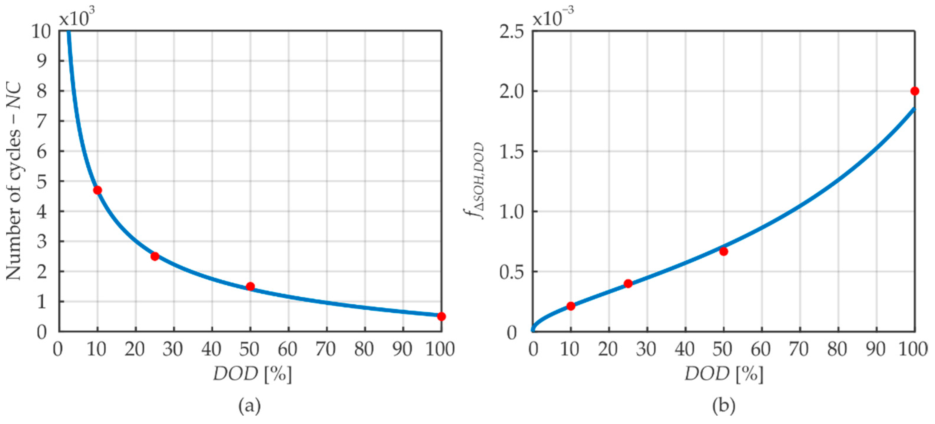
2.1.1. Influence of the Depth of Discharge (DOD)

The depth of discharge can be calculated by the absolute value of the difference between the current and future SOC:

$$DO{D}_{b,t}=\left|SO{C}_{b,t}-SO{C}_{b,t+\mathsf{\Delta }t}\right|.$$

(5)

According to the coulomb counting method, the future SOC of the battery can be estimated by:

$$SO{C}_{b,t+\mathsf{\Delta }t}=SO{C}_{b,t}+\frac{p_{b,n}·\mathsf{\Delta }t}{V_n·SO{H}_{bms}·C_n}·100.$$

(6)

Thus, substituting Equation (6) into Equation (5), one can find an expression of DOD as a function of the power in the battery:

$$DO{D}_{b,t}(p_{b,t})=\left|\frac{p_{b,t}·\mathsf{\Delta }t}{V_n·SO{H}_b·C_n}·100\right|.$$

(7)

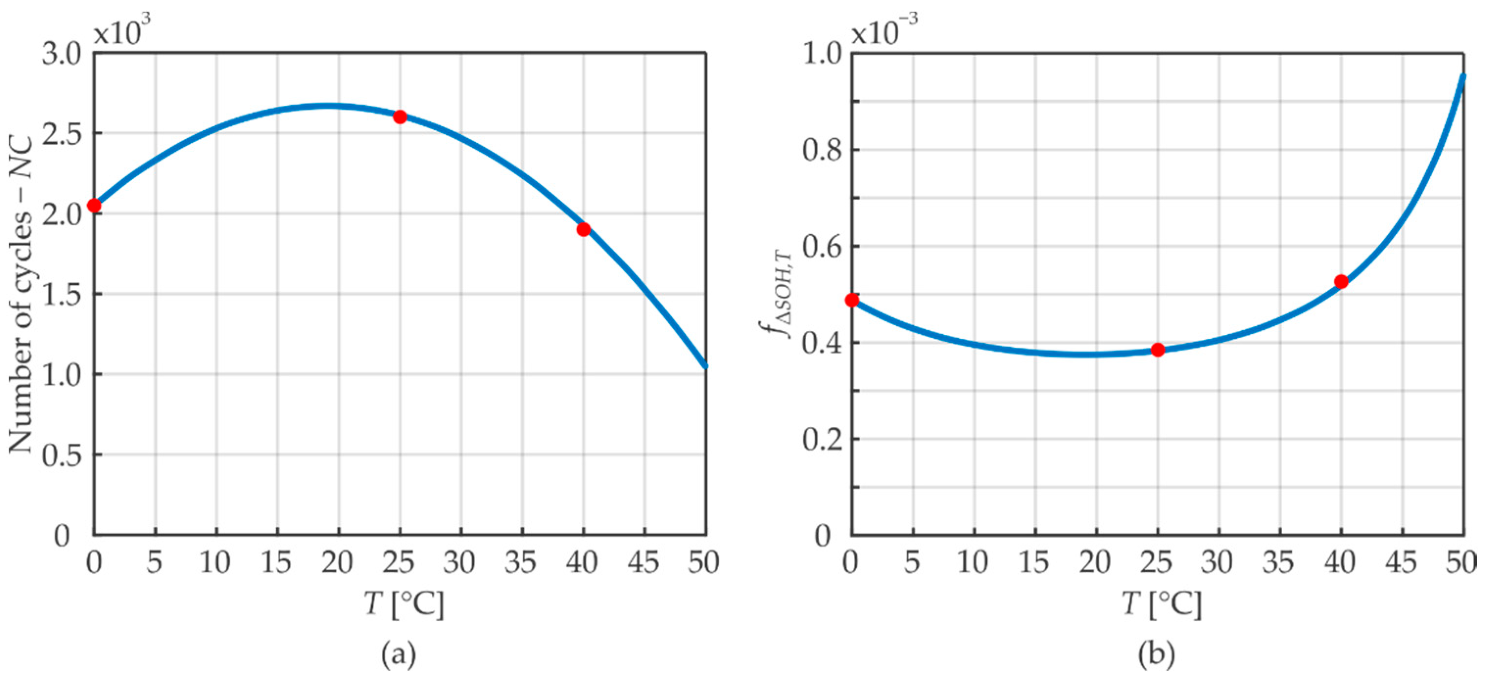
2.1.2. Influence of the Average State of Charge $\left(\overline{SOC}\right)$

The average state of charge can be defined as following:

$${\overline{SOC}}_{b,t}=\frac{SO{C}_{b,t}+SO{C}_{b,t+\mathsf{\Delta }t}}{2}.$$

(8)

Therefore, substituting future SOC, already calculated in Equation (6), into Equation (8), one can find the average state of charge as a function of the battery dispatch power:

$${\overline{SOC}}_{b,t}(p_{b,t})=SO{C}_{b,t}+\frac{p_{b,t}·\mathsf{\Delta }t}{2·V_n·SO{H}_b·C_n}·100.$$

(9)

For the first iteration, the current SOC may be obtained by the BMS estimation:

$$SO{C}_{b,t=0}=SO{C}_{bms},$$

(10)

otherwise, the assumption of a current SOC of 50% is considered a good initial value.

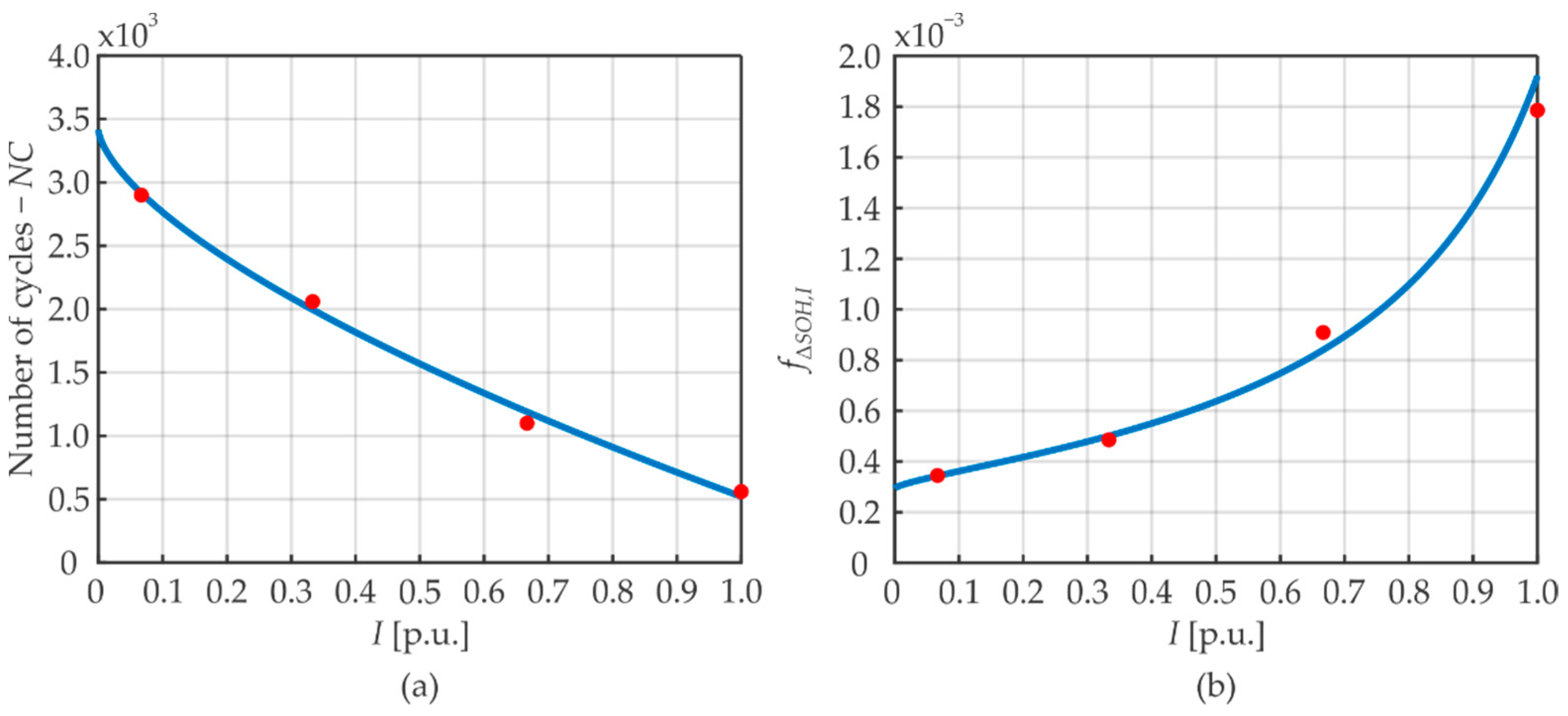
2.1.3. Influence of the Charge and Discharge Currents (I)

The charging and discharging currents are considered to have the same effect over the battery degradation and are normalized by the maximum rated current I_n that the BESS can provide:

$${\widehat{I}}_{b,t}=\left|\frac{I_{b,t}}{I_n}\right|.$$

(11)

In order to find an expression that is a function of the dispatch power p_b,t, the numerator and the denominator of Equation (11) are multiplied by the battery rated voltage V_n, resulting in:

$${\widehat{I}}_{b,t}=\left|\frac{I_{b,t}}{I_n}\frac{V_n}{V_n}\right|.$$

(12)

Thus, considering that I_b,t·V_n = p_b,t and that I_n·V_n = P_n, it is possible to write that:

$${\widehat{I}}_{b,t}(p_{b,t})=\left|\frac{p_{b,t}}{P_n}\right|.$$

(13)

2.2. Lithium-Ion Battery Dataset

According to Equations (3) and (4), in order to identify how the DOD, $\overline{SOC}$, and $\widehat{I}$ affect the degradation of lithium-ion batteries, experimental data are needed. The dataset used in this work was extracted from [23,26]. Ecker et al. [26] provide cycle life measurements for DOD ranging from 10% to 100% and $\overline{SOC}$ ranging from 10% to 95%, while keeping I = 1C, T = 35 °C and $\overline{SOC}$ = 50% or DOD = 10%, as illustrated in Figure 1 and Figure 2, respectively. Conversely, the dataset by Omar et al. [23] contains cycle life measurements for a normalized current $\widehat{I}$ ranging from 0 to 1 p.u., as elucidated in Figure 3. In these figures, the points in red represent the experimental measurements, whereas the fitting curves are obtained as:

$$NC(DO{D}_{b,t})=\mathsf{\alpha }·DO{D}_{b,t}{}^{\mathsf{\beta }}+\mathsf{\gamma },$$

(14)

$$NC({\overline{SOC}}_{b,t})=\mathsf{\alpha }·{\overline{SOC}}_{b,t}{}^2+\mathsf{\beta }·{\overline{SOC}}_{b,t}+\mathsf{\gamma },$$

(15)

$$NC({\widehat{I}}_{b,t})=\mathsf{\alpha }·{\widehat{I}}_{b,t}{}^{\mathsf{\beta }}+\mathsf{\gamma },$$

(16)

using the least squares method in the MATLAB Curve Fitting Tool; the coefficients α, β, and γ for each equation are shown in

Table 1. Values for tuning coefficients of models of lithium-ion degradation impact factors.

Parameter	α	β	γ
DOD	17,390	−0.4052	−2153
$\overline{SOC}$	−1.378	135.01	501.3
$\widehat{I}$	−2894	0.6485	3415
T	−1.717	64.92	2050

. The function relationships described by Equations (14)–(16) and used for curve fitting were based on [22].

Although the effect of temperature is disregard from the proposed model, since all the factors that impact a Li-ion battery cycle life are considered to be independent from each other, there is no impediment in accounting it in the model, if necessary. For example, Figure 4 illustrates the number of cycles as a function of the temperature for the same battery studied in [23]. From such results, one can note that if the operating temperature is kept between 0 °C and 40 °C, the change in the lifetime is not expressive. As before, the points in red represent the experimental measurements, whereas the fitting curve is obtained as

$$NC(T)=\mathsf{\alpha }·T^2+\mathsf{\beta }·T+\mathsf{\gamma },$$

(17)

using the least squares method in the MATLAB Curve Fitting Tool; the coefficients α, β, and γ are also shown in Table 1.

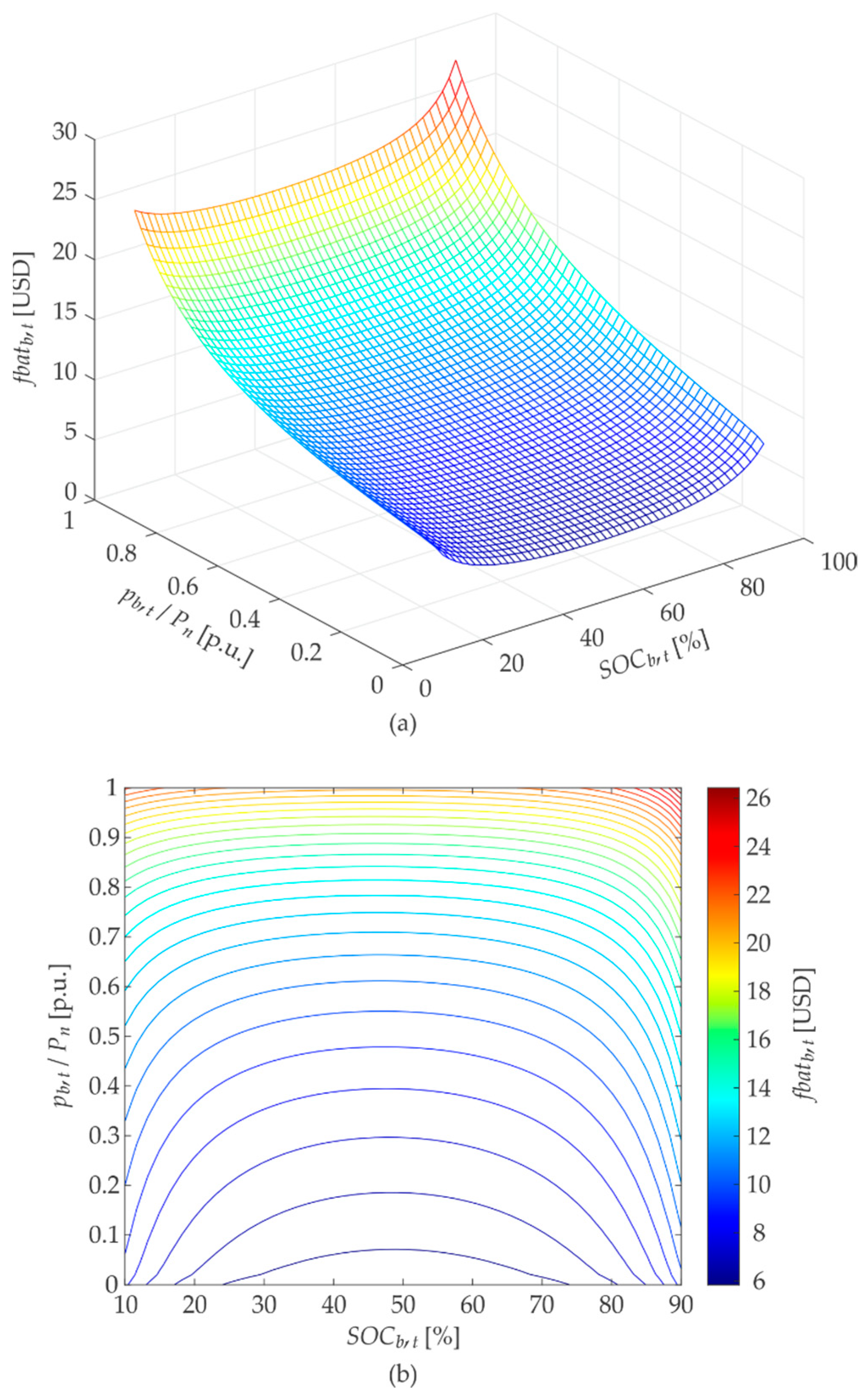
2.3. Battery Degradation Cost Model: Example

To demonstrate the application of the proposed battery degradation cost model, an example is carried out considering a BESS with the parameters listed in

Table 2. BESS parameters.

Variable	Value
Rated power (Pn)	180 kW
Rated voltage (Vn)	1080 V
Rated capacity (Cn)	200 Ah
Investment cost (cb)	USD 400,000.00
Initial SOH (SOHbms)	100%
Discretization interval (Δt)	5/60 h

. Based on them, it can be found by Equation (2) that the rated battery time T_n for a complete charge or discharge is equal to 1.2 h. Therefore, taking into account the empirical curves and equations established in this section, it is possible to plot the cost model as a function of the dispatch battery power and the current state of charge, as illustrated in Figure 5.

2.4. Constraints of the Battery Cost Model

The constraints of the battery cost model described by Equation (1) for a MILP optimization problem are presented in this subsection. Firstly, it is considered that the state of charge of the battery can just vary between a maximum and a minimum value according to:

$$SO{C}_{min}\le SOC\le SO{C}_{max}.$$

(18)

Conversely, the following equations limit the charge pc_b,t and discharge pd_b,t powers to the rated battery power P_n. In Equation (19), the multiplication of P_n by the binary variable bc_b,t ensures that pc_b,t can assume a non-zero value only when the battery is charging. Equation (20) consists of an analogous function, but considering the discharge power pd_b,t and the binary variable bp_b,t. Finally, Equation (21) guarantees that charging and discharging cannot coexist in the same time step.

$$p{c}_{b,t}\le b{c}_{b,t}·P_n,$$

(19)

$$p{d}_{b,t}\le b{d}_{b,t}·P_n,$$

(20)

$$b{c}_{b,t}+b{d}_{b,t}\le 1.$$

(21)

Since two distinct variables pc_b,t and pd_b,t are used to express the dispatch battery power p_b,t during charging and discharging, Equations (7), (10) and (15) can be respectively rewritten as:

$$DO{D}_{b,t}(p{c}_{b,t},p{d}_{b,t})=\frac{\left(p{c}_{b,t}+p{d}_{b,t}\right)·\mathsf{\Delta }t}{V_n·SO{H}_b·C_n}·100,$$

(22)

$${\overline{SOC}}_{b,t}(p{c}_{b,t},p{d}_{b,t})=SO{C}_{b,t}+\frac{\left(p{c}_{b,t}-p{d}_{b,t}\right)·\mathsf{\Delta }t}{2·V_n·SO{H}_b·C_n}·100,$$

(23)

$${\widehat{I}}_{b,t}(p{c}_{b,t},p{d}_{b,t})=\frac{p{c}_{b,t}+p{d}_{b,t}}{P_n}.$$

(24)

Moreover, as the battery degradation cost function is nonlinear, in order to be used in MILP optimization problems, each individual function that represents a change in SOH should be expressed as a piecewise linear function in the form of:

$$f_{\mathsf{\Delta }SOH,x}=\{\begin{array}{c}{a}_1^{T}x+b_1\mathrm{for}{x}_0\le x\le x_1\\ a_2^{T}x+b_2\mathrm{for}{x}_1\le x\le x_2\\ ⋮\\ a_i^{T}x+b_i\mathrm{for}{x}_{i-1}\le x\le x_i\end{array}.$$

(25)

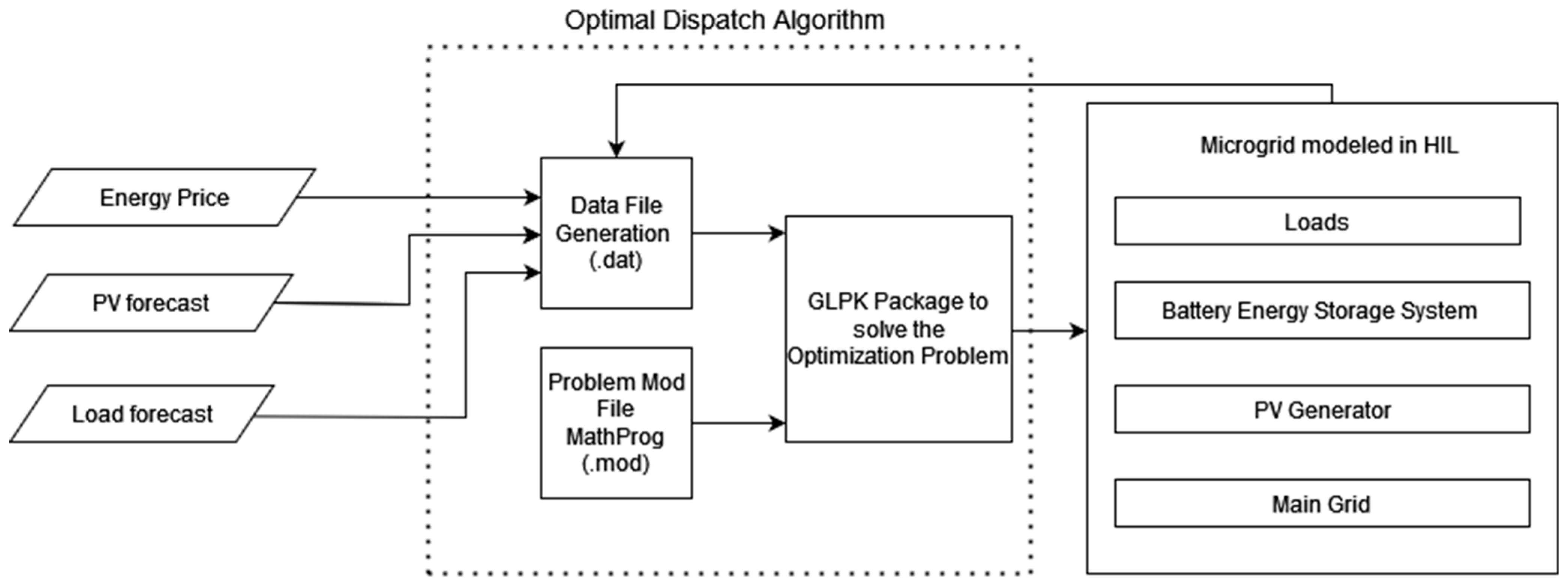
3. Optimization Problem

To evaluate the proposed battery degradation cost model, the same controller described in [27] is implemented. The only difference between the controllers is the novel empirical cost model for BESSs developed in this work. In [27], Makohin et al. designed a microgrid centralized controller (MGCC) that can function as a generic controller for different microgrid configurations. The MGCC is prepared to control microgrids with numerous DERs, such as dispatchable generators, renewable energy sources, energy storage systems, and multiple control loads, in addition to allowing it to operate connected to grid or in islanded mode.

The MGCC has an optimizer based on mixed-integer linear programming, which guarantees the energy cost reduction and reliability in both islanded and connected modes. The controller dispatches resources differently in each mode. Moreover, the main objective of the optimization problem is to minimize the total costs related to the operation of the microgrid. In order to integrate the generation sources and to ensure the lowest leveled cost of energy, each of the microgrid elements has its own cost function. Since the detailed description of the MGCC is beyond the scope of this paper, only a summary of the complete optimization problem is presented in this section.

Objective Function

The optimization problem consists of minimizing the total costs related to the microgrid operation. As presented in Equation (26), besides the battery degradation cost model (fbat_b,t), the operational costs of MGCC includes fuel consumption (fger_g,t), load curtailment (fshd_s,t), maintenance (fman_e,t), buying/selling energy from/to the utility provider (fgrid_t^E), penalty payments for exceeding the power demand agreed with the distribution system operator (fgrid_t^D), and an additional term (frest_t).

$$\begin{array}{c}\min \left(f\right)\\ f={\displaystyle \sum _{t=0}^{nT}\left({\displaystyle \sum _{g=1}^{nFG}fge{r}_{g,t}}+{\displaystyle \sum _{b=1}^{nB}fba{t}_{b,t}}+{\displaystyle \sum _{s=1}^{nSL}fsh{d}_{s,t}}+{\displaystyle \sum _{e=1}^{nE}fma{n}_{e,t}}+fgri{d}_t^E+fgri{d}_t^D+fres{t}_t\right)}\end{array}$$

(26)

The cost function fger_g,t of each dispatchable generator g is given by:

$$fge{r}_{g,t}=A_g·F{C}_g·\mathsf{\Delta }t·p_{g,t}+B_g·F{C}_g·\mathsf{\Delta }t·u_{g,t}+Y{C}_g·y_{g,t}+Z{C}_g·z_{g,t}.$$

(27)

The term fshd_s,t represents the cost of shedding a given load c. In some cases, it is more advantageous to shed loads than continue to supply them, due to the price of buying energy from the utility provider or the lack of internal generation. This cost is defined as:

$$fsh{d}_{s,t}=SD{P}_{s,t}·\left(1-u_{c,t}\right)·PS{L}_{s,t}·\mathsf{\Delta }t.$$

(28)

Each element e has a maintenance cost that is proportional to the number of hours the element is on. Hence, the hourly maintenance cost is represented by:

$$fma{n}_{e,t}=M{C}_e·u_{e,t}·\mathsf{\Delta }t.$$

(29)

The term fgrid_t^E, given by Equation (30), can be positive when the microgrid buys energy from the utility provider, or negative when the microgrid sells energy to the upstream grid.

$$fgri{d}_t^E=\left(B{T}_t·pb{u}_t+S{P}_t·ps{u}_t\right)·\mathsf{\Delta }t.$$

(30)

According to Brazilian regulation, some clients pay a fixed value for the contracted demand rate and, if it surpasses this contracted value, there is an additional cost as a penalty. This process is described by:

$$fgri{d}_t^D=ud{o}_t·O{P}_t·\left(TO{L}_t·Pli{m}_t\right)+O{P}_t·pd{o}_t.$$

(31)

The additional term (frest_t) exhibited in Equation (32) is added to the objective to achieve power balancing, to prioritize outputs while diminishing power deviation, and to keep a given amount of energy within the storage system. The first two terms in Equation (32) apply a high cost to power deficits and excesses; respectively. The third term applies a small cost to power deviations to prioritize smoother dispatches without competing with any one of the terms in Equation (27).

$$fres{t}_t=CD·pde{f}_t+CE·pex{c}_t+{\displaystyle \sum _{d=1}^{nD}\left(IDP·d{p}_{dt}·\mathsf{\Delta }t\right)}$$

(32)

More information about the MGCC optimization problem, as initial conditions, power balance, operational constraints, and events scheduling, can be found in [27].

4. Results

The microgrid considered for the evaluation of the proposed multi-factor battery degradation cost model is shown in Figure 6. As one can note, it is composed of a distribution network, a photovoltaic (PV) system, loads, and the same BESS used as an example in Section 2.3. In this microgrid, the BESS is used for backup generation, storing energy from photovoltaic generation to cover possible demand peaks during periods of higher load, provided that its operating cost is lower than other available sources. To prove the functioning of the proposed mathematical modeling in a simulated platform, tests are carried out in real time using hardware-in-the-loop. The Typhoon HIL 602+ software and hardware are used for this proposal considering the specifications described in

Table 3. Microgrid specifications.

Variable	Value
PV power	99 kW
Loads power	240 kW
BESS power	180 kW
Minimum SOC	10%
Maximum SOC	100%
BESS investment cost (default)	USD 400,000.00
Initial SOC (default)	80%
Contracted demand (default)	200 kW

.

Figure 7 depicts how the proposed algorithm was implemented in this study. The microgrid was modeled from existing Typhoon HIL components. The optimization problem, variables, constants, and parameters were defined in the “Problem Mod File” in MathProg. The values for the problem parameters are generated at each time step in “Data File Generation”. These two files are input into the GLPK package, which solves the optimization problem. In sequential order, the optimal dispatch algorithm receives input data of energy prices, photovoltaic generation forecast, load forecast, and initial conditions of the microgrid. The “Data File Generation” block receives these parameters, creating a .dat file, and inserts it into the solution block. Simultaneously, the block “Problem File Mod” with the .mod file inserts the problem to be solved. The solution of the optimization problem is sent to the microgrid, and, in this specific algorithm, it acts directly on the BESS dispatch. This process is repeated throughout the simulation period considered, which in the case of this study is 24 h.

The tests are accomplished to analyze the battery dispatch in different scenarios and to verify the behavior of the state of charge in each situation. In summary, three test packages are carried out: in the first, a variation is applied in the contracted demand; in the second, a variation is applied in the initial investment of the BESS; and in the third, a variation is applied in the initial SOC. The load and the PV generation profiles are considered the same in all the tests, as shown in Figure 8. The simulation time for each scenario is 24 h, with dispatches and measurements realized every five minutes.

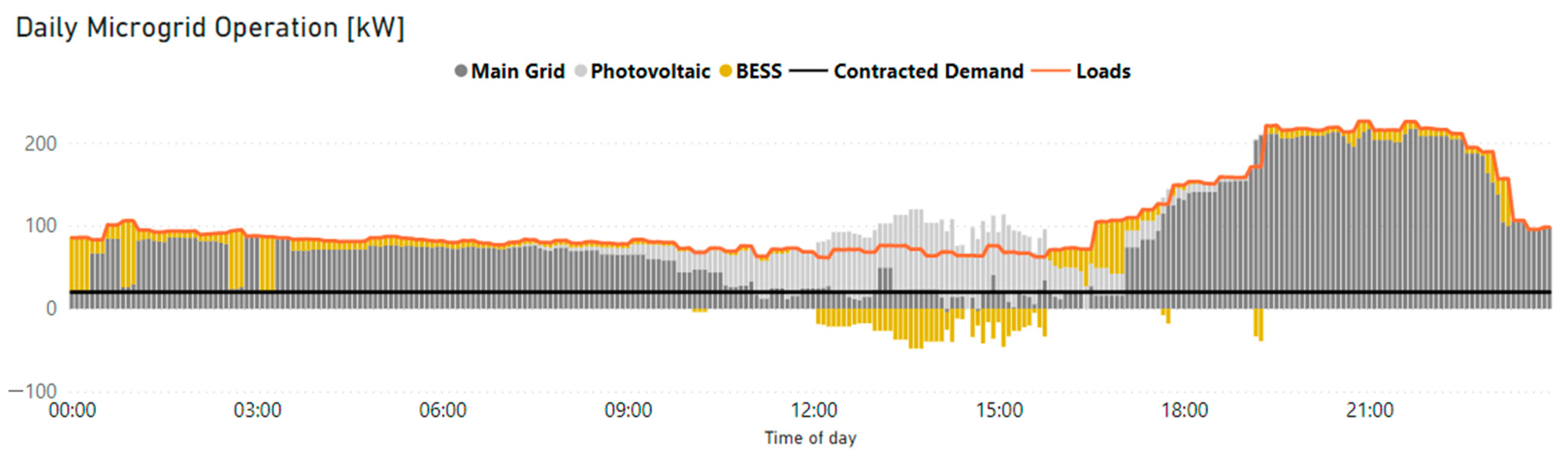
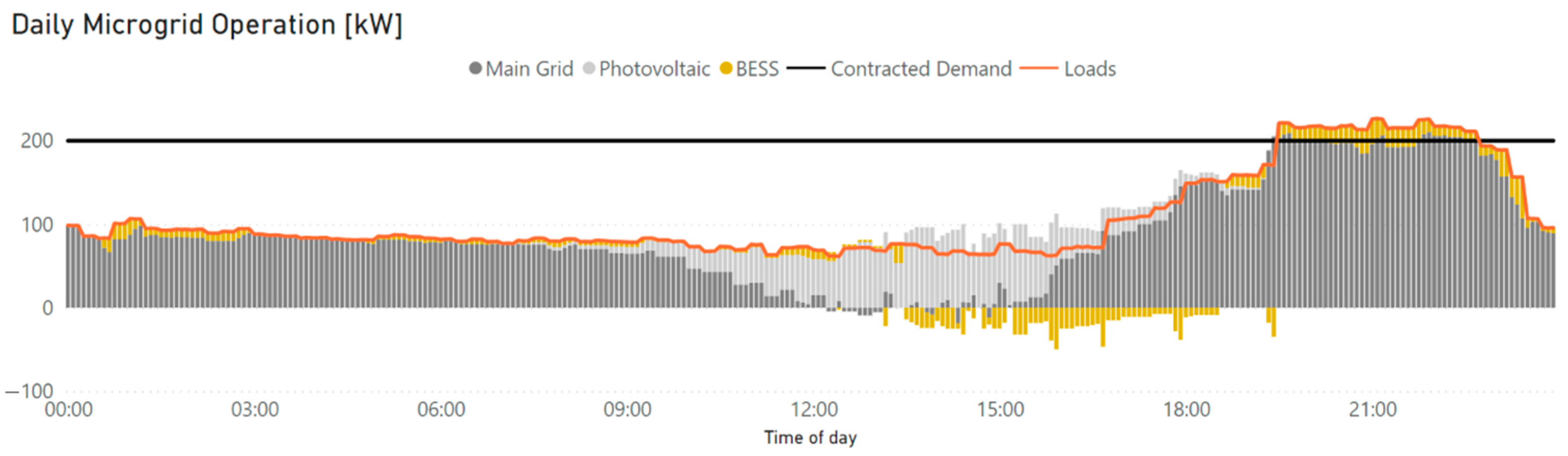
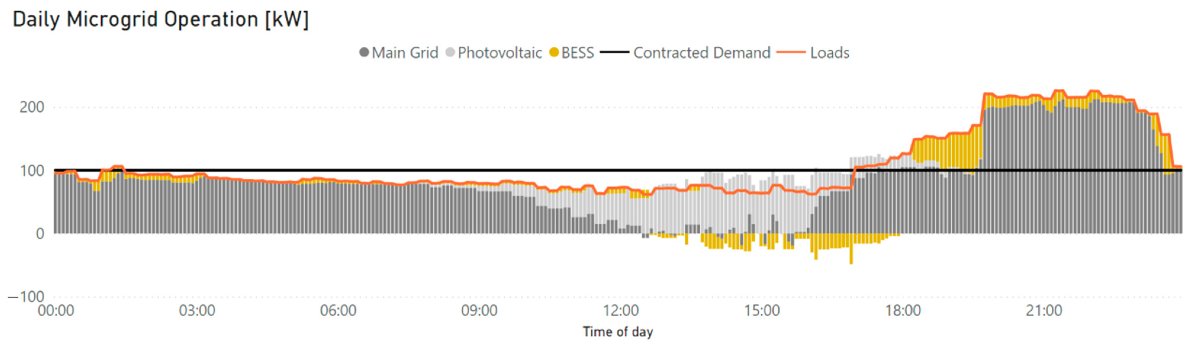
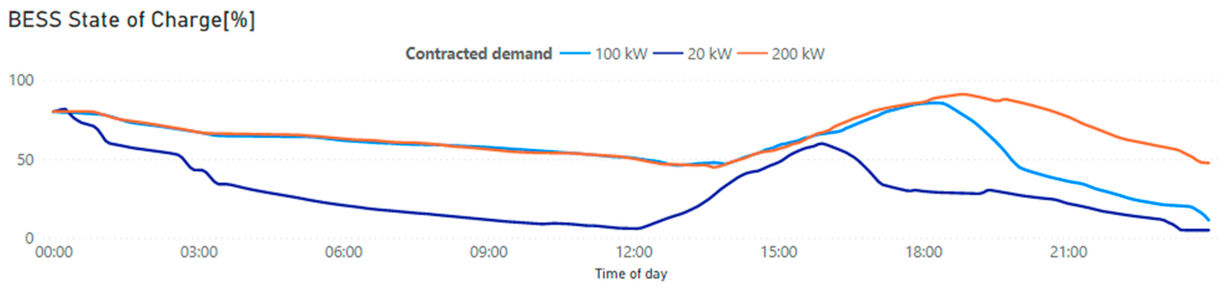
4.1. Contracted Demand

These tests are realized to verify the ability of the microgrid in promoting the peak-shaving, that is, in avoiding peaks in the demand out of the contract. For this proposal, the simulation is achieved to force the load demand to exceed the contracted demand, assumed as 100%, 50%, and 10% of the contracted demand of the real microgrid:

• • Sub scenario 1: Contracted demand of 200 kW (100%).
• • Sub scenario 2: Contracted demand of 100 kW (50%).
• • Sub scenario 3: Contracted demand of 20 kW (10%).

In the results of the daily operation of the microgrid, the power associated to the main grid, photovoltaic system, BESS, loads, and contracted demand are presented in a single graph for each sub scenario evaluated, as shown in Figure 9, Figure 10 and Figure 11, respectively. From these simulations, it is possible to check that the battery is activated to avoid excess demand charges. In summary, the battery bank operates in discharge mode to complement the generation when the load demand exceeds the contracted demand and operates in charge mode to absorb the extra power produced by the PV system when it exceeds the load demanded power.

Figure 12 illustrates how the SOC varies over the time under the three contracted demand values listed before. As observed, when the contracted demand is reduced and there are not enough generation sources to supply the load, the battery is dispatched to avoid exceeding demand. As soon as other generation sources such as PV become available, the battery is recharged to be discharged at peak times. It is worth mentioning that if the contracted demand is much less than the load, the battery is dispatched despite the cost and despite the SOC, as the main objective of the optimization algorithm is supplying the load. Conversely, when the contracted demand is well dimensioned, the battery is dispatched only in the intervals of possible exceeding demand.

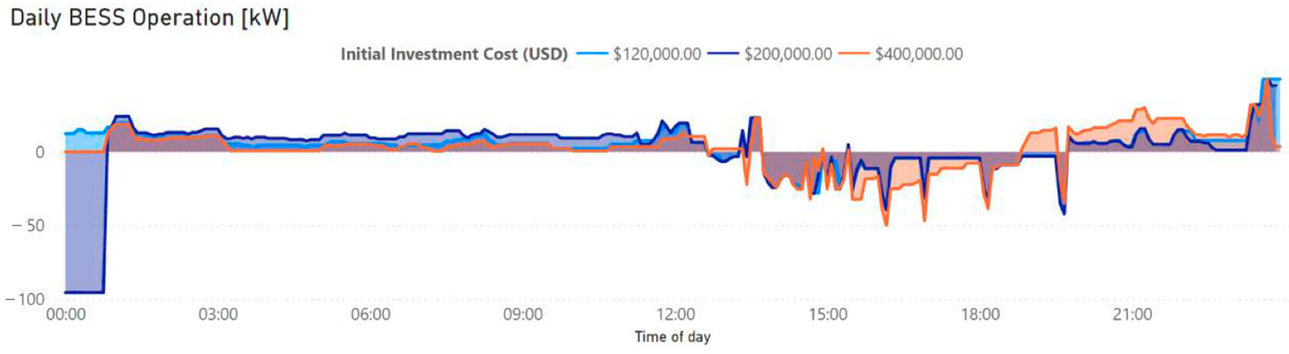
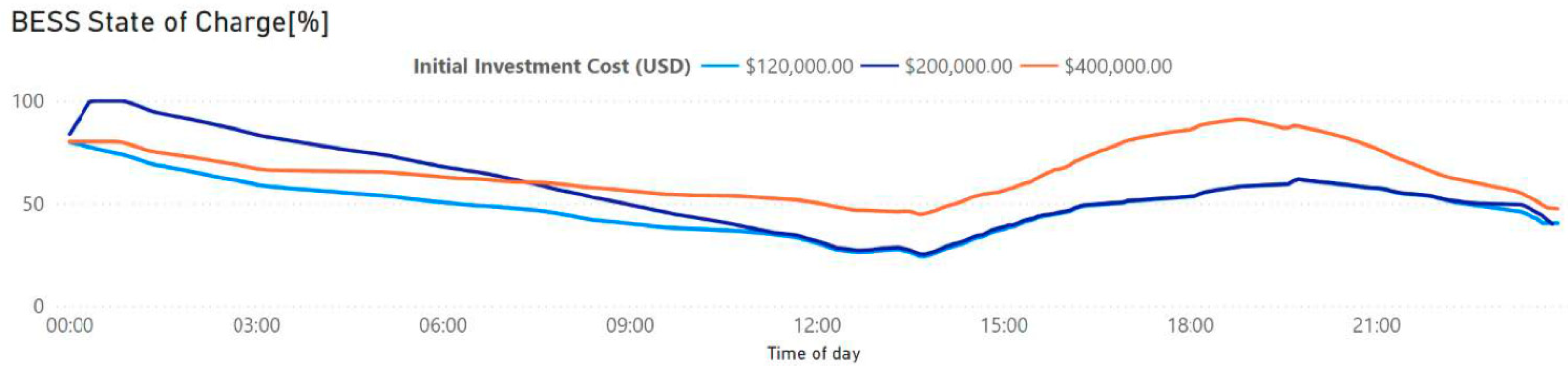
4.2. Investment Cost

The second test consists of analyzing the battery dispatch for different investment costs and other existing generation sources in the microgrid. This test aims to verify if the high cost of investment is an obstacle to the activation of the BESS and what is the investment value that makes the battery bank a viable storage device in the microgrid. Considering that the actual cost of the BESS is USD 400,000.00, three sub scenarios are herein created to investigate how the investment cost impacts battery dispatch:

• • Sub scenario 1: Investment Cost USD 120,000.00.
• • Sub scenario 2: Investment Cost USD 200,000.00.
• • Sub scenario 3: Investment Cost USD 400,000.00.

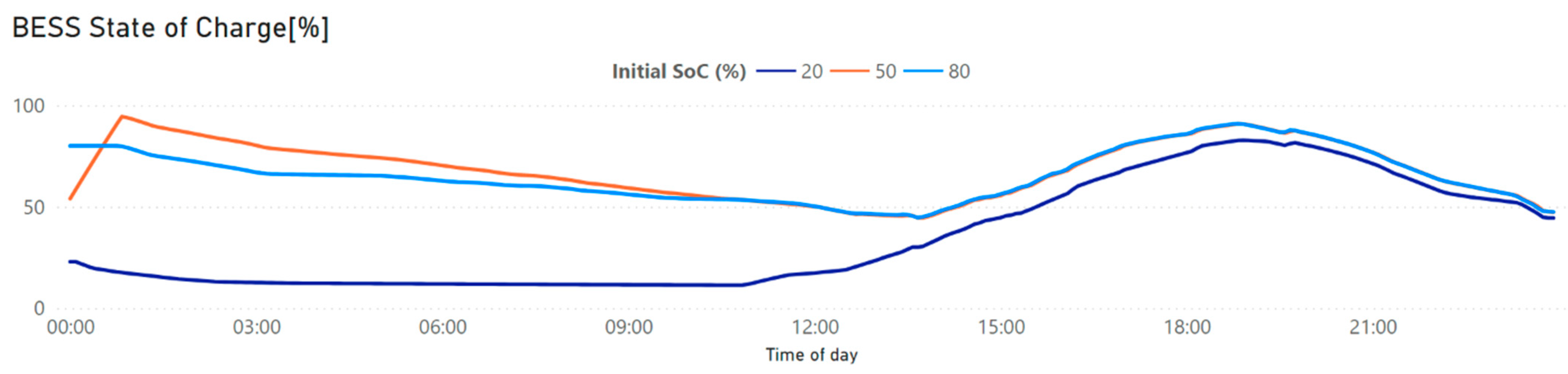
Figure 13 illustrates the results of the BESS charge and discharge powers, and Figure 14 depicts the results of SOC variation by time of day for each value of initial investment cost. In the sub scenario in which the investment cost is the lowest (USD 120,000.00), the battery is already dispatched from the beginning of the microgrid operation, due to its low cost compared to other sources. The average SOC in the daily operation for this scenario is 48.86%.

In the case in which the investment cost is USD 200,000.00, it is observed that the battery is quickly charged as soon as the operation starts. The recharge process is maintained until the SOC rises up close to its maximum value. This scenario presents an average SOC of 57.06% throughout the day. When the investment cost is the higher (USD 400,000.00), the battery is not dispatched immediately after the microgrid starts up. From Figure 14, it is observed that the first discharge takes place only after 45 min of operation. In this case, the SOC remains higher than the other sub scenarios for most of the time, with an average value of 65.87%.

In Figure 13, it can be noted that the investment cost significantly interferes in the battery power dispatch, especially in smoother charge and discharge curves for the highest investment cost. In periods when there is an explicit need to charge the battery (excess of photovoltaic generation) and when it is advantageous to discharge it (the price of energy from the grid is higher), the battery is dispatched in all sub scenarios. However, it is observed that for the highest investment cost, the SOC remains closer to its initial value throughout the day, reinforcing that the higher the investment cost, the lower the power dispatched by the battery.

Moreover, it is worth emphasizing that the battery operation during the day follows the load curve shown in Figure 8. As expected, for most of the period in operation, the BESS does not apply abrupt changes in the SOC. It is also observed that when the battery is charged by the PV generation, the investment cost does not significantly interfere in the battery charging process, since such energy needs to be stored; however, when the investment cost is lower, the battery is activated several times, regardless of the time of day. By contrast, with the highest initial investment cost, the battery is activated only to supply exceeding demand.

4.3. Initial SOC

This test consists of starting the microgrid operation with different initial SOCs. The objective is to verify how much the modeling seeks to balance the SOC value to reduce the battery degradation, whether charging or discharging the battery. The scenarios for this test range from 20% to 80% in relation to the initial SOC with the following sub scenarios:

• • Sub scenario 1: initial SOC of 20%.
• • Sub scenario 2: initial SOC of 50%.
• • Sub scenario 3: initial SOC of 80%.

Figure 15 shows the results of SOC variation by time of day for each initial SOC value during the microgrid operation. When the initial SOC is adjusted to 20%, the battery is not subjected to large cycles of charge before the photovoltaic generation become enough to take it to a high state of charge. During the peak hours, when the photovoltaic generation is unavailable, in order to avoid fines for exceeding demand, the battery is thus discharged to approximately half of the SOC.

When the operation starts with the SOC at 50%, in the first few hours, the battery is charged and the SOC rises to almost 100%, being gradually discharged until the PV generation becomes enough to take it again to a high state of charge. After that, the battery is discharged at peak hours up to an SOC of 50%.

Finally, when the operation starts with the SOC at 80%, there is a gradual discharge of the battery during the first hours, so that the SOC decreases to a level of 50% at 12 pm. After that, the battery is charged with the excess of PV generation to be again discharged at peak hours, in order to complement the extra demand. At the end of the daily operation, the SOC is approximately 50%. It is noticeable that, regardless of the initial SOC of the BESS, during daily operation, while meeting the needs of the load, the SOC converges to a common point, close to the SOC of lowest battery degradation.

Therefore, in view of the analysis of the proposed modeling and the test results, one can conclude that the ideal conditions for battery operation are properly considered to avoid accelerating battery degradation with usage. In summary, the best way to use a Li-ion battery within a microgrid context is working with low power levels of charge and discharge and maintaining the SOC at intermediate values during battery operation.

5. Discussion

The results shown in Section 4 demonstrates the suitable functioning of the proposed model, which makes the microgrid controller avoid the operation of the BESS at low and high SOC values and with large charging/discharging rates, thus not accentuating the wear-out process of the lithium-ion battery. Compared to other state-of the-art solutions, the proposed model is simpler, but properly addresses the most important degradation factors that are typically taken into consideration, as summarized

Table 4. Comparison with other state-of-the-art solutions.

Parameter	[14]	[15]	[18]	[24]	Proposed
Degradation factors	DOD	DOD, P	$\mathit{DOD},I\overline{SOC}$	DOD	$\mathit{DOD},\widehat{I}$ $\overline{SOC}$, nT1
Empirical model	Yes	Yes	Yes	Yes	Yes
Optimization method	MPC	MPC-MIQP	SDP	SDP	MILP
Implementation	Simple	Average	Complex	Average	Simple

¹ Temperature can be easily included.

. In addition, the proposed approach is based on MILP optimization, a consolidated method in the industry and used in a wide range of research areas. Comparatively, the BESS operational cost model developed in [14] was implemented in a microgrid energy dispatch problem using model predictive control (MPC). Other battery cost function, presented in [15], uses hybrid MPC formulation solved by mixed-integer quadratic programming (MIQP), but requires more computational resources. By contrast, refs. [18,24] propose two distinct stochastic dynamic programming (SDP) approaches to optimally operate an energy storage system. Such methods are able to take into account forecast uncertainty, but they are computationally challenging due to the large number of scenarios that have to be considered. The models also require knowledge of the probability distribution of uncertain variables.

6. Conclusions

This paper has proposed an empirical operational cost model for lithium-ion batteries to be applied in power dispatch problems of microgrids. Unlike most of the models previously implemented in microgrids, the proposal considers the degradation of the battery lifetime with use in a simple way, based on the variation in its state of health. Basically, the proposed cost model is a function of battery dispatch power and current SOC, and it uses the information from experimental data relating the number of charge and discharge cycles with the most important factors in the degradation of its lifespan. From real-time simulations of an actual microgrid using a centralized controller that has an optimizer based on mixed-integer linear programming, it is concluded that the proposed battery cost function properly represents the influence of SOC and charge/discharge rate in the lifespan of lithium-ion batteries. In order to evaluate the effectiveness of the proposed cost model, three different scenarios were considered in the hardware emulation. In the first case, the contracted demand was adjusted from 10% to 100% of its real value. The obtained results allow concluding that the time interval in which the battery is dispatched is inversely proportional to the contracted demand. A second scenario investigated the impact of the investment cost, which was adjusted to 30%, 50%, and 100% of the actual price. As a result, the average SOC settled at 48.86%, 57.06%, and 65.87%, respectively, demonstrating that the higher the investment cost, the shorter the time interval in which the battery is dispatched. In the third and last scenario, variations in the initial SOC were investigated. The obtained results show that regardless of the initial value, the final SOC converges to a value close to 50%, which ensures the lowest battery degradation. In light of this, it is concluded that the battery energy storage system behaves as expected to supply the load: charging and discharging according to the operating cost of other microgrid elements and their initial values, and to keep the SOC at adequate levels to reduce battery degradation with use. Future work may include simulation tests or experimental validations considering different configurations of microgrids to better explore the benefits of using the proposed multi-factor battery degradation cost model. Moreover, the method applied in this paper could also be easily extended to other battery technologies.

References

1. Jiayi, H.; Chuanwen, J.; Xu, R. A review on distributed energy resources and microgrid. Renew. Sustain. Energy Rev. 2008, 12, 2472–2483. [Google Scholar] [CrossRef]
2. Shen, J.; Jiang, C.; Li, B. Controllable load management approaches in smart grids. Energies 2015, 8, 11187–11202. [Google Scholar] [CrossRef] [Green Version]
3. Kumar, G.V.B.; Palanisamy, K. A review on microgrids with distributed energy resources. In Proceedings of the Innovations in Power and Advanced Computing Technologies (i-PCAT), Vellore, India, 22–23 March 2019. [Google Scholar] [CrossRef]
4. Xu, Y.; Wang, Y.; Zhang, C.; Li, Z. Coordination of Distributed Energy Resources in Microgrids, 3rd ed.; The IET London: London, UK, 2021; pp. 3–32. [Google Scholar]
5. Katiraei, F.; Iravani, R.; Hatziargyriou, N.; Dimeas, A. Microgrids management. IEEE Power Energy Mag. 2008, 6, 54–65. [Google Scholar] [CrossRef]
6. Choi, M.E.; Kim, S.W.; Seo, S.W. Energy management optimization in a battery/supercapacitor hybrid energy storage system. IEEE Trans. Smart Grid 2012, 3, 463–472. [Google Scholar] [CrossRef]
7. Ku, T.T.; Li, C.S. Implementation of battery energy storage system for an island microgrid with high PV penetration. IEEE Trans. Ind. App. 2021, 57, 3416–3424. [Google Scholar] [CrossRef]
8. Serban, I.; Marinescu, C. Control strategy of three-phase battery energy storage systems for frequency support in microgrids and with uninterrupted supply of local loads. IEEE Trans. Power Electron. 2014, 29, 5010–5020. [Google Scholar] [CrossRef]
9. Tan, X.; Li, Q.; Wang, H. Advances and trends of energy storage technology in microgrid. Int. J. Elect. Power Energy Syst. 2013, 44, 179–191. [Google Scholar] [CrossRef]
10. Hossain, E.; Faruque, H.M.R.; Sunny, M.S.H.; Mohammad, N.; Nawar, N. A comprehensive review on energy storage systems: Types, comparison, current scenario, applications, barriers, and potential solutions, policies, and future prospects. Energies 2020, 13, 3651. [Google Scholar] [CrossRef]
11. Chaudhary, G.; Lamb, J.J.; Burheim, O.S.; Austbo, B. Review of energy storage and energy management system control strategies in microgrids. Energies 2021, 14, 4929. [Google Scholar] [CrossRef]
12. Huang, Z.; Yang, F. Quality classification of lithium battery in microgrid networks based on smooth localized complex exponential model. Complexity 2021, 2021, 6618708. [Google Scholar] [CrossRef]
13. Garmabdari, R.; Moghimi, M.; Yang, F.; Gray, E.; Lu, J. Multi-objective energy storage capacity optimization considering microgrid generation uncertainties. Elec. Power Energy Syst. 2020, 119, 105908. [Google Scholar] [CrossRef]
14. Ahsan, A.; Zhao, Q.; Khambadkone, A.M.; Chia, M.H. Dynamic battery operational cost modeling for energy dispatch. In Proceedings of the 2016 IEEE Energy Conversion Congress and Exposition (ECCE), Milwaukee, WI, USA, 18–22 September 2016. [Google Scholar] [CrossRef]
15. Koller, M.; Borsche, T.; Ulbig, A.; Andersson, G. Defining a degradation cost function for optimal control of a battery energy storage system. In Proceedings of the 2013 IEEE Grenoble Conference, Grenoble, France, 16–20 June 2013. [Google Scholar] [CrossRef]
16. Chen, C.; Duan, S.; Cai, T.; Liu, B.; Hu, G. Optimal allocation and economic analysis of energy storage system in microgrids. IEEE Trans. Power Electron. 2011, 26, 2762–2773. [Google Scholar] [CrossRef]
17. Larsson, P.; Borjesson, P. Cost Models for Battery Energy Storage Systems. Bachelor’s Thesis, KTH School of Industrial Engineering and Management, Stockholm, Sweden, 2018. [Google Scholar]
18. Abdulla, K.; Hoog, J.; Muenzel, V.; Suits, F.; Steer, K.; Wirth, A.; Halgamuge, S. Optimal operation of energy storage systems considering forecasts and battery degradation. IEEE Trans. Smart Grid 2018, 9, 2086–2096. [Google Scholar] [CrossRef]
19. Goebel, C.; Hesse, H.; Schimpe, M.; Jossen, A.; Jacobsen, H.A. Model-based dispatch strategies for lithium-ion battery energy storage applied to pay-as-bid markets for secondary reserve. IEEE Trans. Power Syst. 2017, 32, 2724–2734. [Google Scholar] [CrossRef]
20. Chaturvedi, N.A.; Klein, R.; Christensen, J.; Ahmed, J.; Kojic, A. Algorithms for advanced battery-management systems. IEEE Control. Syst. Mag. 2010, 30, 49–68. [Google Scholar] [CrossRef]
21. Muenzel, V.; Hoog, J.; Brazil, M.; Vishwanath, A.; Kalyanaraman, S. A multi-factor battery cycle life prediction methodology for optimal battery management. In Proceedings of the 2015 ACM Sixth International Conference on Future Energy Systems, Bangalore, India, 14–17 July 2015. [Google Scholar] [CrossRef]
22. Burzynski, D.; Pietracho, R.; Kasprzyk, L.; Tomczewski, A. Analysis and modeling of the wear-out process of a lithium-nickel-manganese-cobalt cell during cycling operation under constant load conditions. Energies 2019, 12, 3899. [Google Scholar] [CrossRef] [Green Version]
23. Omar, N.; Monem, M.A.; Firouz, Y.; Salminen, J.; Smekens, J.; Hegazy, O.; Gaulous, H.; Mulder, G.; Bossche, P.V.; Coosemans, T.; et al. Lithium iron phosphate based battery—Assessment of the aging parameters and development of cycle life model. Appl. Energy 2014, 113, 1575–1585. [Google Scholar] [CrossRef]
24. Nguyen, T.A.; Crow, M.L. Stochastic optimization of renewable-based microgrid operation incorporating battery operation cost. IEEE Trans. Power Syst. 2016, 31, 2289–2296. [Google Scholar] [CrossRef]
25. Murnane, M.; Ghazel, A. A closer look at state of charge (SOC) and state of health (SOH) estimation techniques for batteries. Analog Devices 2017, 2, 426–436. [Google Scholar]
26. Ecker, M.; Nieto, N.; Kabitz, S.; Schmalstieg, J.; Blanke, H.; Warnecke, A.; Sauer, D.U. Calendar and cycle life study of Li(NiMnCo)O2-based 18650 lithium-ion batteries. J. Power Sources 2014, 248, 839–851. [Google Scholar] [CrossRef]
27. Makohin, D.G.; Gloria, L.L.; Zeni, V.S.; Pica, C.Q.; Neto, E.P.A.; Arend, F.G.; Asami, D.Y.; Heraldo, E. Design and implementation of a flexible microgrid controller through mixed integer linear programming optimization. In Proceedings of the 9th IEEE International Symposium on Power Electronics for Distributed Generation Systems (PEDG), Charlotte, NC, USA, 25–28 June 2018. [Google Scholar]
Figure 1. Influence of the depth of discharge DOD: (a) number of cycles and (b) fΔSOH,DOD.
Energies 15 03060 g001
Figure 2. Influence of the average state of charge: (a) number of cycles and (b) fΔSOH,SOC.
Energies 15 03060 g002
Figure 3. Influence of the normalized battery current: (a) number of cycles and (b) fΔSOH,I.
Energies 15 03060 g003
Figure 4. Influence of the temperature: (a) number of cycles and (b) fΔSOH,T.
Energies 15 03060 g004
Figure 5. Proposed battery degradation cost model: (a) 3D plot and (b) contour plot.
Energies 15 03060 g005
Figure 6. Microgrid architecture.
Energies 15 03060 g006
Figure 7. Block diagram for implementation of the optimal dispatch algorithm.
Energies 15 03060 g007
Figure 8. Load and PV generation profiles adopted in all the simulation scenarios.
Energies 15 03060 g008
Figure 9. Daily microgrid operation for a contracted demand of 200 kW.
Energies 15 03060 g009
Figure 10. Daily microgrid operation for a contracted demand of 100 kW.
Energies 15 03060 g010
Figure 11. Daily microgrid operation for a contracted demand of 20 kW.
Energies 15 03060 g011
Figure 12. Variation in the state of charge for each contracted demand.
Energies 15 03060 g012
Figure 13. BESS charge and discharge for each initial investment cost.
Energies 15 03060 g013
Figure 14. SOC variation by time of day for each initial investment cost.
Energies 15 03060 g014
Figure 15. SOC variation by time of day for each BESS initial SOC.
Energies 15 03060 g015