Article

Net Hydrogen Consumption Minimization of Fuel Cell Hybrid Trains Using a Time-Based Co-Optimization Model

1
Shien-Ming Wu School of Intelligent Engineering, South China University of Technology, Guangzhou 511442, China
2
School of Systems Science and Engineering, Sun Yat-sen University, Guangzhou 510006, China
3
School of Advanced Technology, Xi’an Jiaotong-Liverpool University, Suzhou 215123, China
*
Authors to whom correspondence should be addressed.
Energies 2022, 15(8), 2891; https://doi.org/10.3390/en15082891
Submission received: 18 March 2022 / Revised: 8 April 2022 / Accepted: 12 April 2022 / Published: 14 April 2022

Abstract

:
With increasing concerns on transportation decarbonization, fuel cell hybrid trains (FCHTs) attract many attentions due to their zero carbon emissions during operation. Since fuel cells alone cannot recover the regenerative braking energy (RBE), energy storage devices (ESDs) are commonly deployed for the recovery of RBE and provide extra traction power to improve the energy efficiency. This paper aims to minimize the net hydrogen consumption (NHC) by co-optimizing both train speed trajectory and onboard energy management using a time-based mixed integer linear programming (MILP) model. In the case with the constraints of speed limits and gradients, the NHC of co-optimization reduces by 6.4% compared to the result obtained by the sequential optimization, which optimizes train control strategies first and then the energy management. Additionally, the relationship between NHC and employed ESD capacity is studied and it is found that with the increase of ESD capacity, the NHC can be reduced by up to 30% in a typical route in urban railway transit. The study shows that ESDs play an important role for FCHTs in reducing NHC, and the proposed time-based co-optimization model can maximize the energy-saving benefits for such emerging traction systems with hybrid energy sources, including both fuel cells and ESD.

1. Introduction

According to the report published by the International Energy Agency (IEA) in 2017, CO 2 emissions of transportation sector from fuel combustion reached 7.74 billion tons in 2015 [1], of which the rail sector emitted 336 million tons, accounting for 4.34% [2]. One major source of carbon in railway transportation is the trains using fossil fuel directly and indirectly. To minimize fossil fuel consumption in rail transportation, hydrogen is regarded as a feasible and effective solution. As a kind of clean and renewable energy source, hydrogen can greatly reduce carbon emission and the use of non-renewable energy when applied to transportation. As a typical study, Chang et al. established an energy consumption model based on traffic data from various parts of China, demonstrating that the use of hydrogen fuel cells in transportation represents one of the future development trends, especially in public transportation [3]. The feasibility of fuel cell hybrid trains (FCHTs) had been verified in many studies [4,5]. Although the technical cost is relatively high at the current stage, FCHTs have some advantages over electric trains and diesel trains on railways with lower traffic density [6]. In this case, optimizing train control and energy management of hybrid power systems is one of the main focuses in the study of cost reduction.
The optimal train speed trajectory with minimum traction energy demand exists when a train is running between two adjacent stations based on Pontryagin’s maximum principle (PMP) [7,8]. Based on PMP, the optimal train control modes, i.e., accelerating with maximum acceleration rate, braking with maximum braking rate, cruising, and coasting, and their optimal sequences, can be obtained for one inter-station journey. The PMP-based method obtains the optimal solution via solving the co-state function and it is referred to as the “indirect method” [9]. Another commonly used method is the direct method, which transforms the optimal control problem into a mathematical programming problem, typically represented by pseudospectral method, mixed integer linear programming (MILP), and other mathematical programming methods. In [10], both pseudospectral and MILP methods were proposed to optimize the train control strategies under fixed arrival time. The MILP method can easily improve the model to add other engineering constraints [11]. In addition, dynamic programming (DP) and various heuristic algorithms are also used to locate the optimal train control strategies. DP simplifies a complex problem by decomposing it into simpler sub-problems in a recursive manner. In [12], two heuristic algorithms, ant colony optimization and genetic algorithm, and DP were applied to search the speed trajectory, and the results show that the optimum train trajectory cannot be solved analytically, and numerical methods must be used.
While the train optimal control of FCHTs shares similar characteristics with other rail vehicles, the optimization of the speed trajectory of FCHTs can generally locate the minimum energy demand from the traction system. However, there are two important traction components of FCHT, i.e., energy storage devices (ESDs) and fuel cell, that deserve further study when the onboard energy management strategies are studied. For FCHTs, the characteristics of ESDs should be considered along with the train optimal control strategies, especially when the ESDs are charging and discharging along with the train control strategies such as braking and motoring. In [13], Snoussi et al. used sliding mode control for energy management, which well absorbed the peak power in fuel cell trains. In the past few years, many studies have focused on the the ESDs applied to electric trains to increase the recovery of regenerative braking energy and to improve the system performances. In [14], ESD is equipped on the electric train to increase the use of regenerative energy and stabilize the voltage, and the DP algorithm-based heuristic is designed to find the optimal speed trajectory. In [15], Wu et al. employed the MILP to locate the optimal train control, and the results indicated that ESD has a significant influence on the speed trajectory of electric train.
On the one hand, the characteristics of ESDs play an important role in train control; on the other hand, the nonlinear characteristics of fuel cell efficiency impose further complexity on the onboard energy management and train controls. The energy management strategy determines the power distribution between fuel cell and ESDs, and has a significant impact on the total consumption of hydrogen fuel. In recent years, there have been many methods to optimize energy management strategies, such as state machine strategy, fuzzy logic control, equivalent consumption minimization strategy, etc. [16,17]. Current studies are conducted with the fixed power–demand [18]. In [19], the convexity of the specific consumption curve is applied to improve the fuel economy. Based on a suggested power–demand curve, a scalable energy management strategy is designed. In [20], an online extremum-seeking method is used to estimate the maximum efficiency and maximum power points of the fuel cell. In [21], a fixed speed trajectory in FCHTs is divided into four states: traction, braking, coasting, and station parking, and then the power distributions between fuel cell and the supercapacitor (SC) are distributed through a multi-mode equivalent energy consumption method. The work in [22] extended to multiple fuel cells, and realized the power splits among multiple fuel cells by means of the equivalent fitting circle method, and optimized the power output of SC by means of equivalent energy consumption method. In [23], Yan et al. optimized the speed trajectory with the aim of achieving the minimum energy consumption, then determined the hybrid system control strategy based on minimum hydrogen consumption. In [24], a rule-based energy management strategy was proposed to maximize regenerative braking energy recovery. In [25], the braking process speed trajectory was obtained based on motor characteristic curve, supercapacitor capacity, maximum acceleration, and other information to ensure that the supercapacitor can obtain more regenerative braking energy, but this method does not consider the efficiency of the fuel cell. In [26], sequential optimization was applied to improve the potential of fuel efficiency, which develops a speed-smoothing strategy first then optimizes the battery charge based on the smoothed speed profile. However, the train control strategies impose direct impacts on the traction energy demand and are not included in the energy management process in the sequential optimization process. This may undermine the effectiveness of the optimization methods.
In the research area of hydrogen reduction for FCHTs, some recent papers proposed different methods in co-optimizing both train control strategies and onboard energy management concurrently. In [27,28], PMP and DP were combined to solve this problem by applying the Hamiltonian as the objective function of DP, but its application was inevitably constrained by ”the curse of dimensionality” and the boundary-value problem. In [29], Peng et al. proposed dynamic programming for co-optimization of train driving cycles and energy management for fuel cell trains. The parallelization of DP has been proposed to reduce computation time. However, when the dimension of the state variables in the dynamic programming model increases, the calculation time of the model will increase significantly due to the characteristics of the algorithm characteristics. In [30], Jibrin et al. solved the co-optimization of both energy management and speed trajectory by formulating a convex optimization model using convexity relaxation techniques which greatly improved the calculation efficiency, but convex optimization requires that every constraint in the model is convex, which affects the flexibility of the model. The above-mentioned state-of-the-art studies adopted DP and convex programming in dealing with the co-optimization, and they all promoted the advantages of applying co-optimization for FCHTs.
However, it can be seen from the above research that the existing research on co-optimization mainly adopts dynamic programming [27,28,29] and convex optimization [30]. Different from the existing methods of co-optimization, a new method is proposed in this paper to solve the co-optimization problem, and the hydrogen-saving mechanism of a fuel cell train is studied by using the co-optimization model. In addition, the energy-saving potential of regenerative braking process and enhancement of fuel cell efficiency during application by taking the advantage of the hybridization of both fuel cell and onboard ESDs needs further investigation. A detailed overview and comparison of the existing research and this paper are given in Table 1.
This paper aims to develop a time-based MILP model, which has a relatively short computational time, to find the optimal speed trajectory and energy management strategy simultaneously to minimize the net hydrogen consummations. The contributions of this paper are as follows.
(1)
A time-based co-optimization model based on MILP for FCHT is proposed to tackle the intrinsic nonlinear efficiency characteristics of fuel cell and convert the traditional energy-saving problem into a more realistic hydrogen-saving one. The train control, namely, the train speed trajectory, and energy management between two adjacent stations are optimized simultaneously to guide the autonomous driving.
(2)
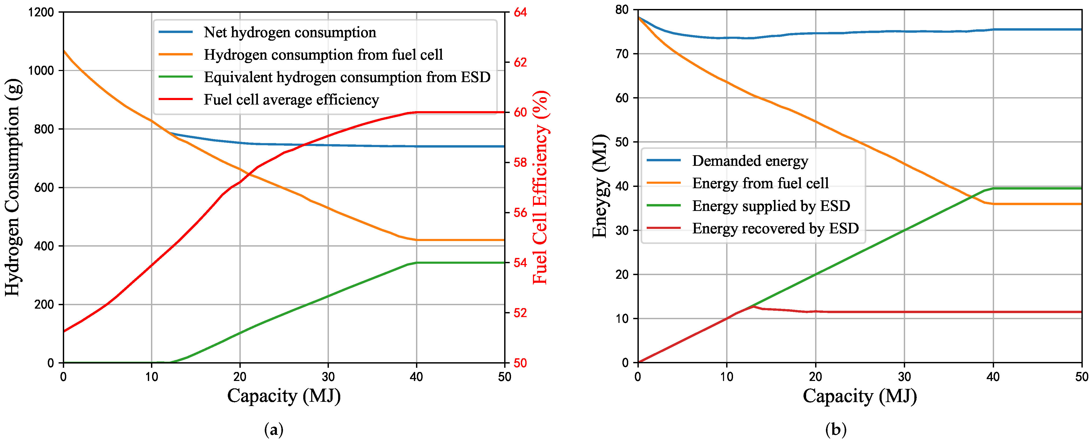
The impact of capacity of ESD on the hydrogen consumption has been studied for FCHTs, and the corresponding hydrogen-saving mechanisms are explored with the quantitative simulation results, giving an insightful analysis and discussion on the mutual influence on optimal train operation.
The remainder of the paper is organized as follows: Section 2 proposes the mathematical model in detail, including motion model, energy flow model, piecewise linearization, and objective modeling. Section 3 analyzes the impact of ESD capacity on hydrogen consumption and gives the comparison between co-optimization and sequential optimization under different scenarios. Section 4 concludes the study and discusses the future research directions.

2. Methods

2.1. Motion Model

In this paper, the train is modeled as a particle. In [31], a distance-based MILP model is established to find the optimal speed trajectory of a FCHT, where Δ d i are known parameters and Δ t i are variables, as shown in Figure 1. However, heavy computational loads are required when calculating the output power from the fuel cells, P i = E i / t i . It is noted that both E i and t i are both variables and the linearization of the ratio in the MILP model results in computational complexity due to the large magnitude difference and nonlinear relationship between the energy consumption and the corresponding time in the i t h distance segment. Alternatively, this paper proposes a time-based MILP model to avoid this nonlinear relationship, where Δ t i are known parameters and Δ d i are variables. The train speed at each time instance is determined by the MILP model, and it is considered that the train accelerates or decelerates uniformly in each time segment. As shown in Figure 1, the speed trajectory is divided into N time segments, and the train travels through each segment with a fixed period of time, Δ t i , the length of which can vary according to different case scenarios. The distance traveled in the i t h segment is denoted by Δ d i .
In this study, we assume that the train travels at a constant acceleration or deceleration rate during each time period; thus, Δ d i can be calculated by (1).
Δ d i = v i , a v e Δ t
where v i , a v e is the average speed in i t h segment denoted by (2).
When the total running time and travel distance are T and D, respectively, the number of the segments is N = T / Δ t . Therefore, the total distance of the train should meet the constraint (3).
v i , a v e = ( v i + 1 + v i ) / 2
i = 1 N Δ d i = D .
When the train is running, it will be subjected to the resistance from the rotating shaft, rail, and air drag. In the model, the train resistance is modeled by the the Davis equation, Equation (4):
f i , d r a g = A + B v i , a v e + C v i , a v e 2
where f i , d r a g is the drag force in the i t h segment. A, B, and C are Davis coefficients.
To ensure safe operation of the train and the comfort of the passenger, the acceleration and deceleration cannot exceed their maximum value. The values for maximum acceleration and deceleration can follow the data from dealing with similar train operation optimization problems [10].
A b , m a x ( v i + 1 v i ) / Δ t = a i A a , m a x
where A a , m a x and A b , m a x are the maximum acceleration and deceleration rate, respectively.
The speed of the train should not exceed its speed limit, v i , L , at each time instance t i . The definition of v i , L is given by (29).
v i v i , L .

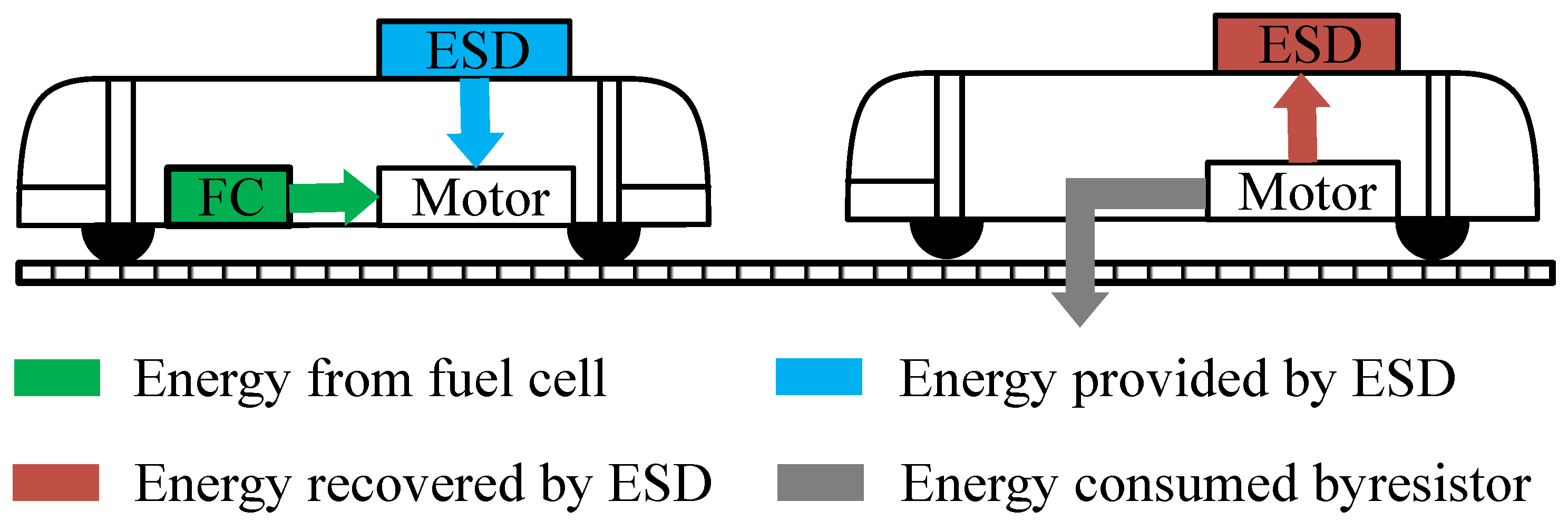
2.2. Energy Flow Model

Similar to normal train operations, there are four control strategies of FCHTs: traction, cruising, coasting, and braking. When the train is in traction or cruising, the hydrogen fuel cell and ESD provide the power to the train. During coasting, there is no need to provide energy to the train, and kinetic energy is used to overcome resistance. Because the fuel cells cannot absorb the regenerative braking energy (RBE) when the train is braking, ESD is used to recover the RBE. A simple schematic diagram of a fuel cell hybrid system is shown in Figure 2. This paper will optimize the train energy distribution strategy from the perspective of energy flow.
The conservation laws of energy in traction and braking process are modeled by (7) and (8), respectively. There are four types of energy: the traction energy or braking energy by the electric machines, the change of potential energy and kinetic energy of the train, and the energy converted to heat due to the drag force.
E i , s e g η m M g Δ h i 1 2 M ( v i + 1 2 v i 2 ) f i , d r a g Δ d i 0
E i , s e g / η m M g Δ h i 1 2 M ( v i + 1 2 v i 2 ) f i , d r a g Δ d i 0
where M is the total mass of the train, g is the acceleration rate due to gravity, Δ h i is the altitude difference of i t h segment, E i , s e g is the traction or braking energy of the motor in the i t h segment, and η m is the efficiency of the motor. When E i , s e g is greater than zero, it means the train is in traction or cruising mode, and E i , s e g η m is smaller than E i , s e g / η m . (7) will be applied while (8) is relaxed. When E i , s e g is equal to zero, the train is coasting; when E i , s e g is less than zero, the train is braking, and E i , s e g η m is greater than E i , s e g / η m . (8) will be applied while (7) is relaxed. The relaxation corresponding to different train state is listed in Table 2. In addition, it should be noted that during the braking mode, the mechanical braking and electrical braking can both be applied. In this case, (8) will reach “>” when mechanical braking and regenerative braking happens at the same time, transforming the kinetic energy to heat and electricity, and it will reach “=” when only regenerative braking energy happens, transforming the kinetic energy to electricity.
In order to model the physical characteristic constraints of the motor, the operation of the motor should conform to its traction and braking characteristics. During motoring, the sum of the output power of the fuel cell and ESD should be less than the maximum traction power of the motor. During braking, the braking power should not exceed the maximum braking power of the motor. These related constraints are as follows:
F b , m a x Δ d i η m E i , s e g F t , m a x Δ d i / η m
P b , m a x Δ t η m E i , s e g P t , m a x Δ t / η m
where P t , m a x and P b , m a x are the maximum traction power and maximum braking power respectively. F t , m a x and F b , m a x are maximum traction force and maximum braking force, respectively.
The energy flow during each time segment can be modeled by using a binary variable λ i (11).
λ i ( E i , f c + E i , d i s η E S D ) ( 1 λ i ) E i , c h / η E S D E i , s e g
E t r a c = i = 1 N ( E i , f c + E i , d i s )
E f c = i = 1 N E i , f c
where η E S D is efficiency of ESD. E t r a c is the energy required for train traction, which can be calculated by (12). E i , f c is the energy from hydrogen fuel cell, E i , d i s is the energy from ESD. E i , c h is the energy recovered by ESD at the i t h segment. E f c is the energy provided by the fuel cell throughout the operation. When the train is braking, regenerative energy is generated and charged into ESD.
λ i is a binary variable; it guarantees that the charging and discharging of ESD will not occur simultaneously, and the fuel cell will not charge ESD directly, as constrained by (14)–(16). L is a sufficiently large number that it is greater than the maximum energy that the fuel cell and ESD can provide in Δ t . When λ i = 1 , ESD discharges and the fuel cell operates, and the constraints (15) and (16) are relaxed, and E i , c h is equal to 0. When λ i = 0 , ESD is charged and the fuel cell stops operating, and the constraint (14) is relaxed.
0 E i , c h ( 1 λ i ) L
0 E i , d i s λ i L
0 E i , f c λ i L .
In this study, the state of energy (SOE) is used to denote the energy state of ESD; a similar modeling was adopted in [32], and its value is the current available energy of ESD divided by its total capacity (17). To ensure that the total charged and discharged energy does not exceed the capacity of ESD, (18) should be satisfied.
S O E i = E i n i + j = 1 i E j , c h j = 1 i E j , d i s E c a p
0 S O E i 1
where E i n i is the initial available energy in ESD. E c a p is the capacity of ESD.
For the output power of the fuel cell and ESD, they should be less than the rated power, and the charging power of ESD should be less than the rated charging power. These constraints are given by
E i , f c P f c , m a x Δ t
E i , c h P d , m a x Δ t
E i , d i s P c , m a x Δ t
where P f c , m a x is the maximum output power of the fuel cell, and P d , m a x and P c , m a x are the maximum discharging and charging power of ESD, respectively.

2.3. Piecewise Linearization Using Special Ordered Set Type 2 (SOS2)

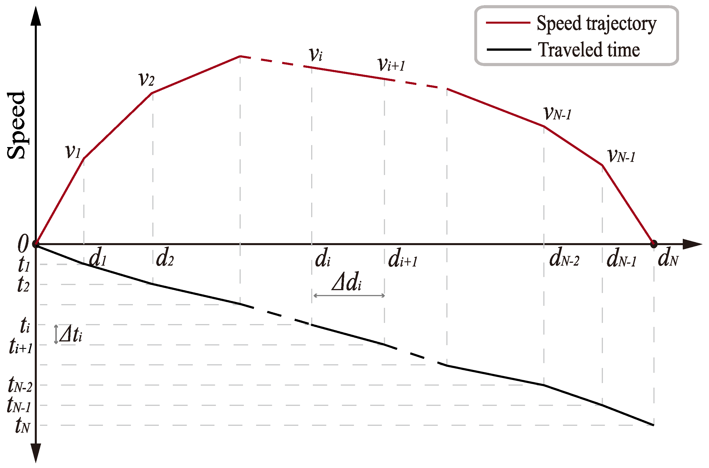
2.3.1. Speed-Related Variables

In the MILP model, a series of variables related to speed are included, and the relationship between them is nonlinear. Piecewise linearization (PWL) is applied to handle nonlinear relationships, which can represent a nonlinear function with a series of nonnegative variables of the special ordered set type 2 (SOS2), among which only two adjacent ones can be greater than 0, with the total sum of all variables equal to 1 [33]. To linearize the nonlinear constraints in (4) and (7), a series of ascending numbers, C 1 , C 2 , , C K , are defined to represent any speed within the range from v 0 to v N . As a result, the decision variables v i 2 , the approximation of the speed v i , v i , a v e , and v i , a v e 2 , can be expressed by
v i 2 = j = 1 K C j 2 α i , j
v i = j = 1 K C j α i , j
v i , a v e = v i + v i + 1 2 = j = 1 K C j β i , j
v i , a v e 2 = j = 1 K C j 2 β i , j
where α i , j and β i , j are variables of SOS2. The two variable of SOS2 should satisfy the constraints (26) and (27).
j = 1 K α i , j = 1 , j = 1 K β i , j = 1
0 α i , j 1 , 0 β i , j 1 .
Using the preset points, e.g., C 1 , C 2 , , C K and C 1 2 , C 2 2 , , C K 2 , along any nonlinear 2D curve to present the relationship between two variables, it is possible to apply a variable of SOS2 to approximate the PWL relationship in between. In this section, we present the PWL modeling technique to approximate the quadratic relationship between the instant speed v i and its square v i 2 . In the following sections, our discussion will be focused on identifying the preset points, and the detailed modeling technique can be referred to the one using SOS2 variables discussed in this section.

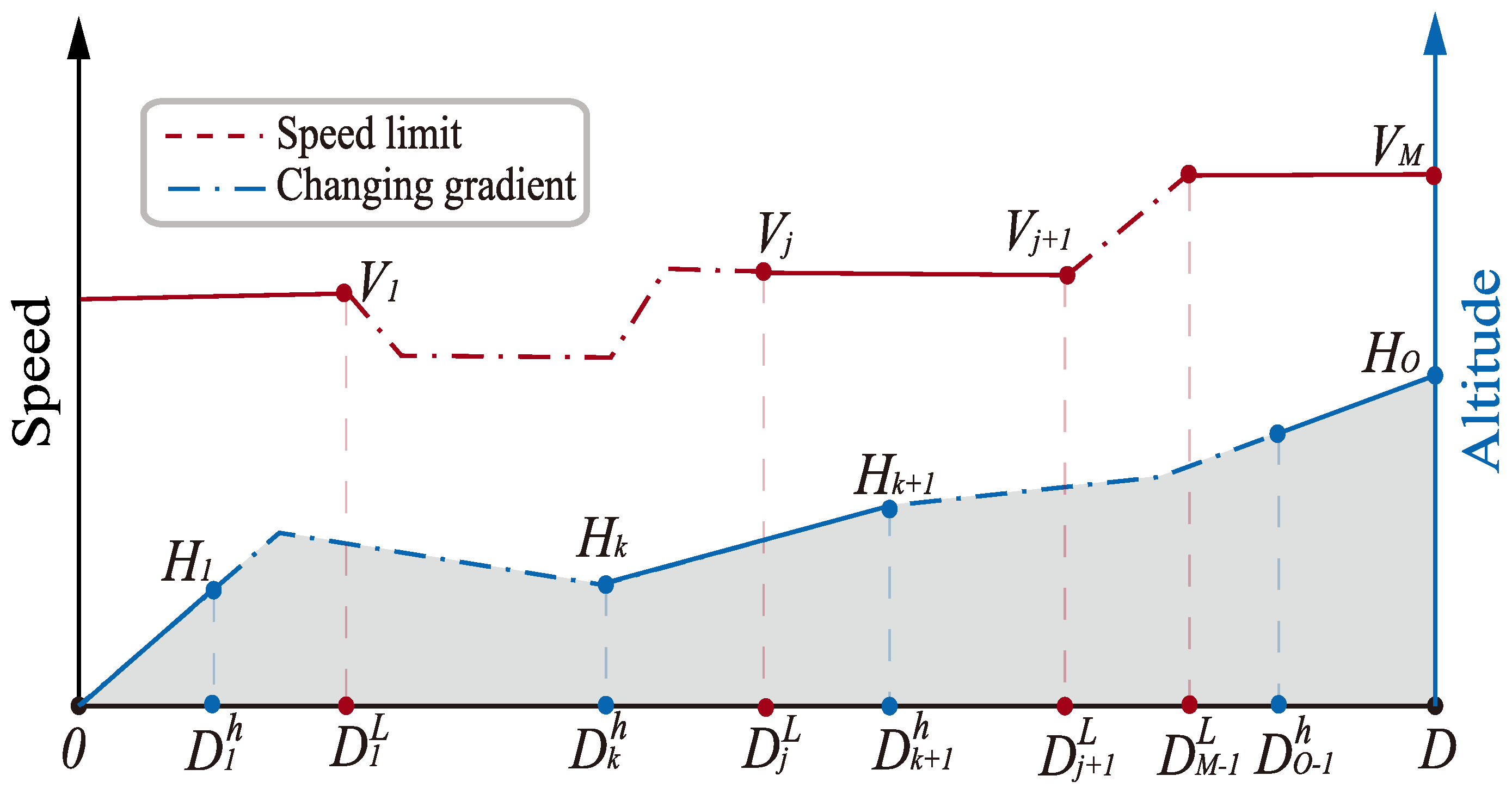
2.3.2. Speed Limit and Altitude

For speed limits, as shown in Figure 3, the speed at each point cannot exceed the speed limit of the red curve, but speed limit generally is based on distance, so d i is used to indicate the position of the train (28) where i = 2 , 3 , , N , and d 1 = Δ d 1 .
d i = j = 1 i Δ d j .
By introducing PWL, the maximum speed limit at each point, v i , L , can be formulated by
v i , L = a j l d i + b j l , d i [ D j L , D j + 1 L )
a j l = V j + 1 V j D j + 1 L D j L , b j l = V j V j + 1 V j D j + 1 L D j L D j L
Let α i , j v be the SOS2 variable sets to formulate the piecewise linear relationship of the speed limit for each d i ; the calculation can be conducted as shown in (31).
v i , L = V j + 1 V j D j + 1 L D j L d i + V j V j + 1 V j D j + 1 L D j L D j L = j = 1 M 1 D j α i , j v , j = 1 M 1 α i , j v = 1
where j = 0 , 1 , 2 , , M 1 , D 0 L = 0 , D M L = D . The speed at the distance of D is limited by
v N , L = V M .
Similarly, the piecewise linear function of altitude, f h , can be obtained. It is shown in Figure 3, and the gradient of d i can be calculated by
h i = a k h d i + b k h , d i [ D k h , D k + 1 h )
a k h = H k + 1 H k D k + 1 h D k h , b k h = H k H k + 1 H k D k + 1 h D h h D k h
Let α i , k h be the SOS2 variable sets to formulate the piecewise linear relationship of the altitude for each d i ; the calculation can be conducted as shown in (35).
h i = H k + 1 H k D k + 1 h D k h d i + H k H k + 1 H k D k + 1 h D h h D k h = k = 1 O 1 D k α i , k h , k = 1 O 1 α i , k h = 1
where k = 0 , 1 , 2 , , O 1 , D 0 h = 0 , D O h = D . The altitude at distance D is given as follows.
h N = H O
Then, the gradient difference can be obtained by
Δ h i = h i + 1 h i .

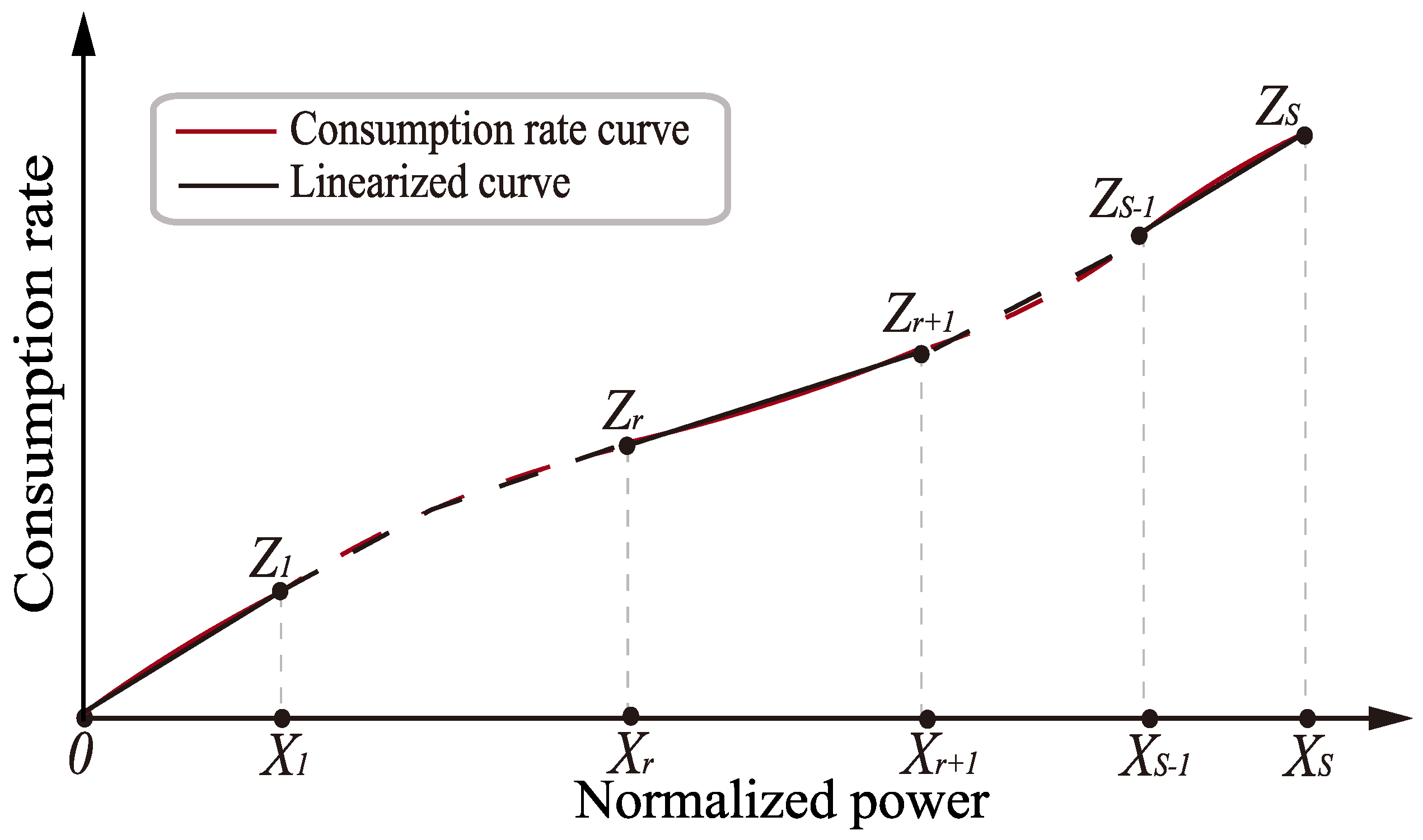
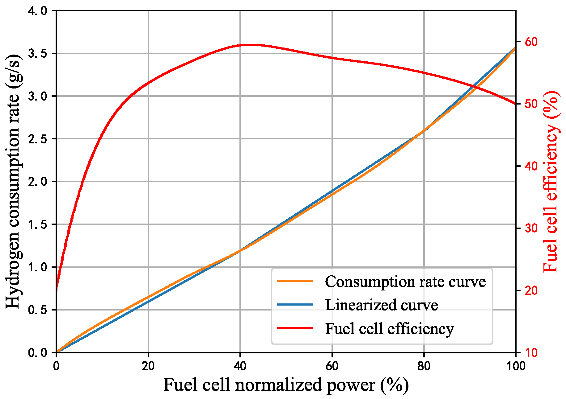
2.3.3. Hydrogen Efficiency

In this model, hydrogen consumption rate is used to calculate the final consumption of the hybrid system. Based on the fuel-cell efficiency, the hydrogen consumption rate can be calculated by
C r i f c = P i , f c H · η i , f c
where P i , f c and η i , f c are the power output and efficiency of the fuel cell in i t h segment, H is the combustion heat value of hydrogen, and C r i , f c is the corresponding hydrogen consumption rate whose modeling is further illustrated in Figure 4.
The hydrogen consumption rate for fuel cell is closely related to its output power, and it is normally represented with respect to the normalized power [29,34]; thus, in this proposed method, the hydrogen consumption rate can be modeled as follows:
C r i , f c = a r f c θ i , f c + b r f c , θ i , f c [ X r , X r + 1 )
a r f c = Z r + 1 Z r X r + 1 X r , b r f c = Z r Z r + 1 Z r X r + 1 X r X r
Let α i , r C be the SOS2 variable sets to formulate the piecewise linear relationship of the hydrogen consumption rate; the calculation can be conducted as shown in (41).
C r i , f c = Z r + 1 Z r X r + 1 X r θ i , f c + Z r Z r + 1 Z r X r + 1 X r X r = r = 1 S 1 X r α i , r C , r = 1 S 1 α i , r C = 1
where r = 0 , 1 , 2 , , S 1 , X 0 = 0 , X S = 100 , θ i , f c is the fuel cell normalized power which can be calculated by
θ i , f c = P i , f c P f c , m a x · 100 % .
When the normalized power is X S , the hydrogen consumption rate is given by
C r N , f c = Z S .
In the time-based MILP model, the power of the fuel cell is obtained by
P i , f c = E i , f c / Δ t .

2.4. Co-Optimization and Sequential Optimization Model

For a hydrogen fuel cell, the consumption of the hydrogen fuel in i t h segment, m i , can be calculated by (45). The total consumption of hydrogen fuel, m f c , can be calculated by (46).
m i , f c = C r i , f c Δ t
m f c = i = 1 N m i , f c .
To evaluate the value of hydrogen consumption, we apply an equivalent conversion of the energy discharged from or charged into ESD to hydrogen consumption, i.e., the hydrogen consumed by the fuel cell operating at the fixed efficiency to produce the same amount of energy discharged from ESD. In this paper, we take the maximum efficiency of the fuel cell, η f c , m a x .
m i , E S D = P i , E S D · Δ t H η f c , m a x
where m i , E S D is the equivalent hydrogen consumption of ESD in the i t h segment. P i , E S D is the power of ESD in the i t h segment. The value of P i , E S D is calculated by
P i , E S D = E i , d i s E i , c h Δ t .
In the whole operation process, the RBE recovered by ESD can be calculated by (49), and its equivalent hydrogen can be calculated by (50).
E c h = i = 1 N E i , c h
m c h = E c h H η f c , m a x .

2.4.1. Co-Optimization

The objective function of co-optimization is applied in the co-optimization model, as shown in (51), which is to minimize the net hydrogen consumption (NHC) in the whole operation process.
N H C = min v i , P i , f c , P i , E S D i = 1 N ( m i , E S D ( v i , P i , E S D ) + m i , f c ( v i , P i , f c ) )
where v i , P i , f c , and P i , E S D are the decision variables. The demanded power curve is determined by v i , and the energy management strategies are determined by P i , f c and P i , E S D , both of which help the train operate at the minimum hydrogen consumption are obtained simultaneously.

2.4.2. Sequential Optimization

On the other hand, the objective function of the sequential optimization is introduced as follows. Compared with the control strategy of electric or fossil-fuel vehicles, hybrid electric vehicles (HEV) are challenging, since there are more control states resulted by the nonlinear characteristics of fuel cells and the charge and discharge states of ESD. Sequential optimization can reduce the computing load and memory usage. The objective equations of sequential optimization are as follows:
  • Step 1: Speed trajectory optimization
    The first step is to obtain the speed trajectory with the aim of minimizing net energy consumption (NEC) of the motor. Namely, we take (52) as the objective function. Thus, it needs to be subject to constraints related to the solving speed trajectory, (1) ∼ (10) and (22) ∼ (35).
    N E C = min v i i = 1 N E i , s e g ( v i )
    Subject to: (1)–(10) and (22)–(35) where v i is the decision variable.
  • Step 2: Energy management optimization
    The second step is to optimize the energy management with the aim of minimizing the net hydrogen consumption (NHC). In this step, the speed trajectory is obtained during the first step, determining the energy demand of the motor, E i , s e g . Thus, the second step can be described as (53).
    N H C = min P i , f c , P i , E S D i = 1 N ( m i , E S D ( P i , E S D ) + m i , f c ( P i , f c ) ) Subject to : ( 11 ) ( 21 )   and   ( 36 ) ( 47 )
    where P i , f c and P i , E S D are the decision variables.

3. Results

The modeling parameters of FCHT in this paper are listed in Table 3 with references to the design proposed in [29]. The global optimizer used in this study to solve the MILP model is GUROBI9.0 [35]. In this section, the optimization results of the time-based MILP model are analyzed. In this study, the supercapacitor is applied as ESD for FCHT. The energy density of the supercapacitor is in the range of 2.5∼15 kWh/t [36], and it also has a relatively high efficiency, generally around 95% [37]. In this paper, the energy density is selected to be 10 kWh/t, i.e., 36 MJ/kg. At the same time, the converters (such as GTO and IGBT), motors, and gear system also have energy losses. As mentioned in [38], the efficiency of them are in the range of 98.5∼99.5%, 90∼94%, and 96∼98%, respectively. In this paper, the efficiency of the converters and gear system is incorporated in the motor efficiency, set as 90%.
Proton exchange membrane fuel cells (PEMFCs) are widely used for their stability and efficiency. A power–efficiency curve of a PEMFC stack is shown in Figure 5. The power–efficiency model does not consider the characteristics of current and auxiliary system in detail, but only considers the relationship between fuel cell efficiency and output power. When the output power of the fuel cell is low, the efficiency is low due to the factors related to the operation of the air compressor, cooling, and humidifying system. The efficiency decreases due to the increase of current at high load demand. It is noted that since the power–efficiency relationship shows that the lowest efficiency of the fuel cell is 20% with the output power of it being 0, when the efficiency is 20%, the fuel cell can be regarded to be in the non-working status.

3.1. The Impact of ESD Capacity on Hydrogen Consumption

In this section, the effect of ESD on the equivalent hydrogen consumption of a hybrid power system is studied based on the co-optimization model. Two case studies, i.e., Case 1 and Case 2, are proposed to model the FCHT with and without ESDs, respectively. In Case 1, the capacity of ESD is assumed to be 0 MJ to indicate that the FCHT is not equipped with ESD, and ESD capacity in Case 2 is set to be 40 MJ. Comparison of results between the two cases is shown in Table 4. The initial SOE for ESD in Case 2 is 1.
In Figure 6a, the optimized speed trajectories are demonstrated. It can be seen that the speed trajectory varies when ESD is introduced. The acceleration of Case 1 without ESD is smaller, so a longer acceleration phase and higher coasting speed are required to meet the time constraint and this leads to more traction energy needed for Case 1.
Power splits between fuel cell and ESD are shown in Figure 6b, where the solid line represents the optimization results when ESD capacity is 40 MJ, and the dashed line represents the results without ESD. It can be seen from this figure that the fuel cell in Case 2 outputs 100 kW for all working hours except for 150 kW for 10 to 20 s. ESD provides extra power so that fuel cell in Case 2 can work with a higher efficiency. In addition, in Case 1, the RBE is consumed directly as heat while the RBE is recovered by 11.51 MJ, which allows 12.83% equivalent hydrogen consumption to be saved in Case 2.
It can be seen that the net hydrogen consumption of the two is significantly different. The net hydrogen consumption of Case 2 can obtain a saving of 29.58% compared with Case 1. This comparison shows that the introduction of ESD can reduce net hydrogen consumption from two aspects. On the one hand, ESD assists fuel cells to avoid high-power but low-efficient working states; on the other hand, RBE can be recovered to improve the energy efficiency.
To show the detailed mechanism on how the fuel cell and ESD influence each other, the relationship between fuel cell and ESD capacity is studied for this hybrid power system. Optimization results with the varied ESD capacities by using the proposed model are shown in Figure 7a,b. Note that the initial SOE for ESD is 1.
As can be seen from Figure 7a, as ESD capacity increases, net hydrogen consumption decreases, and this trend is particularly evident in the low capacity, from 0 to 13 MJ. At this stage, the equivalent hydrogen consumption of ESD is 0. It can be seen from Figure 7b that the reason is that the energy provided by ESD is equal to the energy recovered. This indicates that at low capacity, the increase in recovered regenerative braking energy can significantly reduce net hydrogen consumption.
When ESD capacity increases from 13 to 40 MJ, the net hydrogen consumption of the train decreases slowly, while the equivalent hydrogen consumption of ESD increases and the hydrogen consumption of the fuel cell decreases. From the perspective of energy flow, the hybrid power system is more inclined to use the energy in ESD due to the higher energy efficiency of ESD. This is reflected in the fact that with the increase of ESD capacity, ESD provides more energy for traction, which allows the fuel cell to work at a higher efficiency and obtain a higher average efficiency. In addition, although the net hydrogen consumption decreases slowly, it can be seen from Figure 7b that the demanded traction energy of the train increases slowly, while the RBE also slightly decreases. This also reflects the higher energy efficiency of the hybrid power system.
It is noted that when ESD capacity is greater than 40 MJ, the net hydrogen consumption remains unchanged, and it can be seen from Figure 7a that the fuel cell average efficiency is 60%, which is the maximum value. Since the efficiency of ESD in this model is a constant, and in this model, the maximum efficiency of the fuel cell, which is 60%, is used to equate the energy provided by ESD to hydrogen consumption, the energy conversion rate of the system reaches the highest, and the net hydrogen consumption of the system is the minimum. Therefore, when the objective is to minimize hydrogen consumption, 40 MJ can be considered as the optimal ESD capacity of the system.

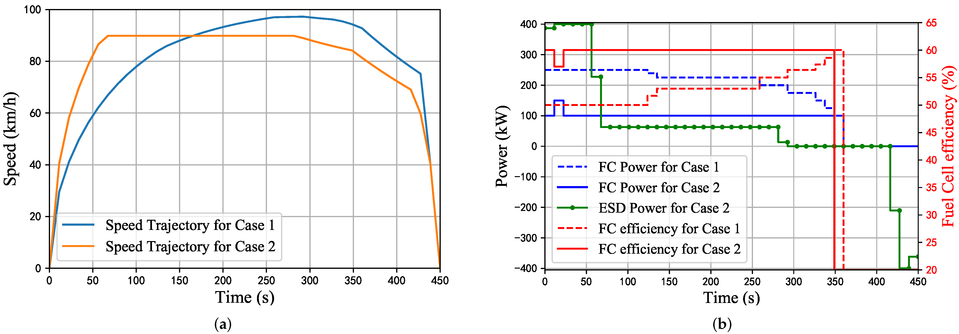
3.2. Case Study on Flat Track

Section 3.2 and Section 3.3 are the comparison between co-optimization and sequential optimization. In this section, a simple case is conducted to explore the difference between the two methods on a flat track to avoid the effect of gradient and speed limit on traction or braking power. The capacity of ESD in this case is selected as 40 MJ and its initial SOE is 1, and the travel distance and time are 10 km and 450 s. The performance comparison between the two is listed in Table 5, where Case 2 and Case 3 are based on co-optimization and sequential optimization, respectively.
The speed trajectory and motor power are shown in Figure 8a. The solid line and the dashed line represent the results of co-optimization and sequential optimization, respectively. It can be seen that the speed trajectory of sequential optimization can be divided into four stages, acceleration with maximum acceleration, cruising, coasting, and deceleration with maximum deceleration, which meets the optimal control theory, and it should be noted that the train of Case 3 which is based on sequential optimization accelerates to the cruise speed with the maximum traction power, while Case 2 does not. Figure 8b represents the power output of the fuel cell and ESD. From this figure, it can be seen that ESD of Case 2 and Case 3 have reached the maximum power output in the acceleration stage, and the power difference at this stage is only reflected in the output power of the fuel cell.
In Figure 8b, it is shown that in the acceleration stage, the fuel cell efficiency of Case 3 is 55%, but for Case 2, except for the fuel cell output power of 11 s to 22 s, which is 150 kW when the efficiency of fuel cell is 58%, the output power of the other acceleration time is 100 kW when the efficiency of fuel cell is 60%. That is to say, the fuel cell in Case 2 worked at the point of higher efficiency during the whole acceleration process. As shown in Table 5, even though the fuel cell of Case 3 provides less traction energy, the hydrogen consumption of the fuel cell is still higher, which means that the average efficiency of the fuel cell in Case 3 is lower than the one in Case 2.
It can be seen from Table 5 that the calculation time of sequential optimization is short and it has an advantage in terms of net energy consumption, i.e., 62.28 MJ. In the meantime, the result by co-optimization consumes 64.27 MJ of net energy. However, since the efficiency of the fuel cell is improved during the operation obtained by co-optimization, the net hydrogen consumption in the co-optimization results is lower, saving 3.1% compared to the one in Case 3. The sequential optimization first optimizes the speed trajectory with the minimum energy consumption, so the NEC is less than co-optimization. In terms of hydrogen consumption, the nonlinear characteristics of fuel cell efficiency are considered during optimization in the co-optimization model proposed in this paper. This method allows energy management to actively change the speed trajectory accordingly, thereby changing the corresponding power–demand curve to further improve the energy conversion efficiency of the fuel cell. As a result, the fuel cell efficiency in the operation obtained by the co-optimization result is higher than the one in the results of sequential optimization.

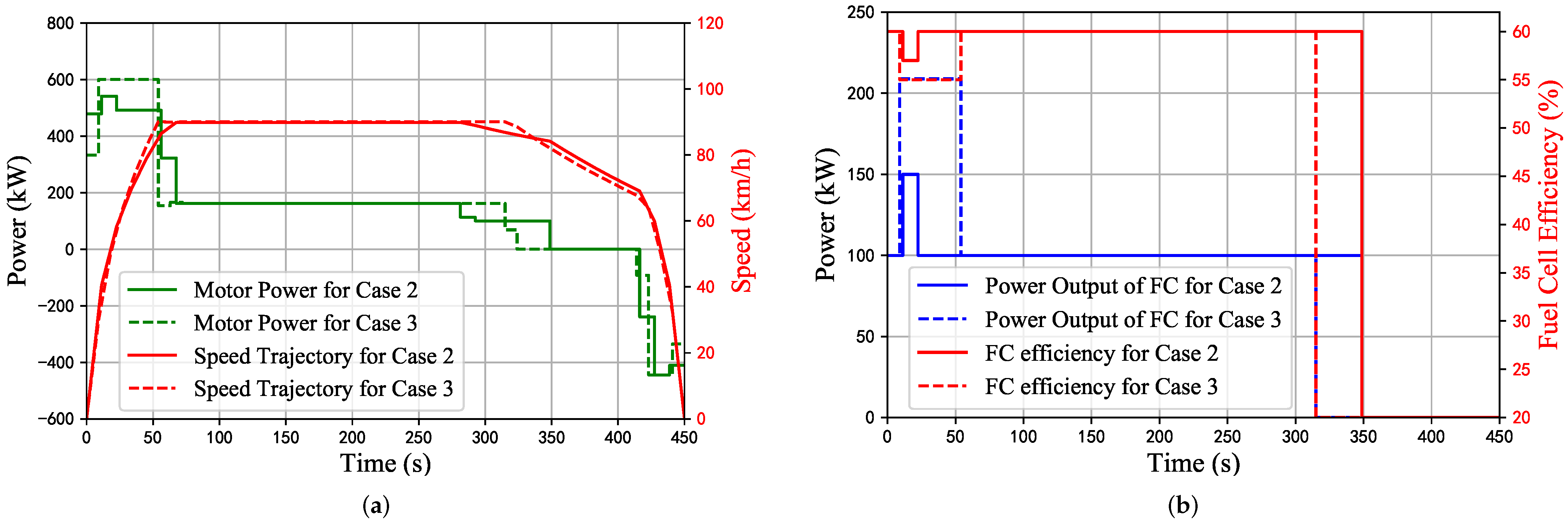
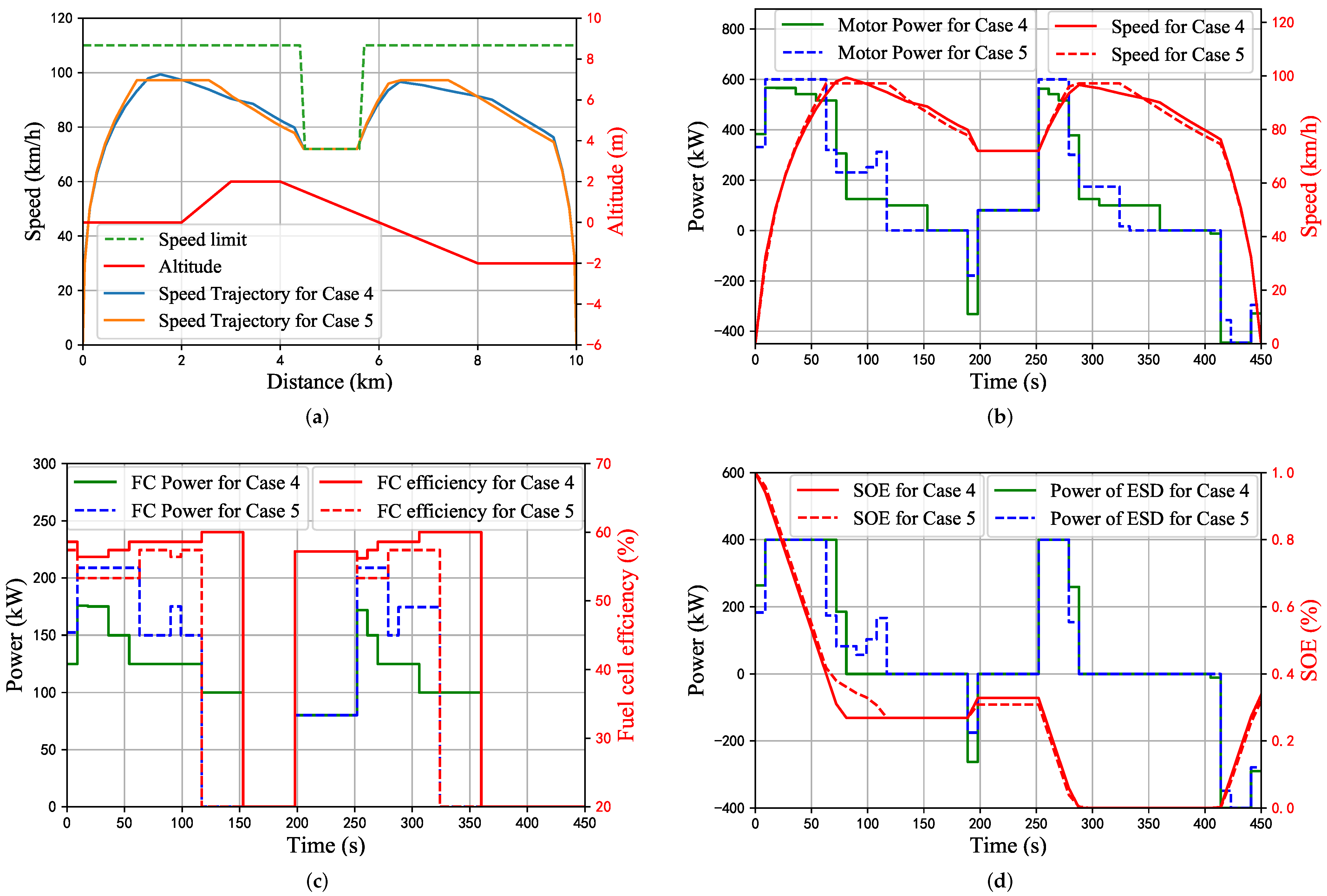
3.3. Case Study with Speed Limits and Gradients

The above cases are carried out on the assumption that there is no speed limit and gradient in the journey. However, in the real-world railway operations, there are speed limits and gradients along the journey. In this case, ESD capacity, travel distance, and time were 40 MJ, 10 km, and 450 s, respectively. The initial SOE of ESD is 1. Case 4 and Case 5 indicate co-optimization and sequential optimization, respectively. The geographic information is shown in Figure 9a; a speed limit section, an uphill area, and a downhill area are added.
With extra constraints of gradients and speed limits introduced, from the speed trajectory profiles presented in Figure 9b, it can be seen that the train cruises at 72 km/h in 196 s to 450 s in the speed limit area, and the train of sequential optimization is still accelerating with maximum acceleration, which requires higher traction power. There are still some differences in the two acceleration phases; the traction power of the train in Case 5, from 0 to 62 s and 252 s to 285 s, is 600 kW, which means that the train has the maximum acceleration.
As shown in Figure 9c, the efficiency in Case 4 in general is higher than the one in Case 5 due to a better energy management on the train load demand to enable a higher working efficiency of the fuel cell. As can be seen from Table 6, the net hydrogen consumption in Case 4, i.e., co-optimization, is reduced by 6.48% compared with that in Case 5, i.e., sequential optimization.
Different from the case study on the flat railway track, the speed trajectories of the two methods are different in the cruising phase. It can be seen from the discharge of ESD of Case 4 in Figure 9d that ESD discharges all the available energy during the acceleration process of the train, so the train in Case 4 is not running at a constant cruise speed to avoid the high fuel cell power. From the energy-efficiency point of view, the train needs higher power during acceleration, so ESD is more inclined to discharge during the acceleration process to increase the train’s speed, and this will support the fuel cell to work in states with higher efficiency.
It can be seen from the above case studies that the power split strategy of both the fuel cell and ESD is determined by the algorithm itself but not preset by rules. In the model, only the total energy demand or generation of the train is considered, and by conducting the optimization, the power and energy split of the fuel cell and the supercapacitor can be configured by the model automatically to achieve the objective of minimizing the hydrogen consumption.

4. Conclusions and Future Work

In this paper, we establish a time-based MILP co-optimization model to optimize the train control and energy management simultaneously to minimize the net hydrogen consumption. Based on this model, two problems are discussed. The first is the relationship between ESD capacity and net hydrogen consumption in a hybrid power system. The results show that ESD can reduce net hydrogen consumption by up to 29.58% in the proposed case study. It provides extra power to enable the fuel cell to work at the point of higher efficiency, leading to a significant reduction of net hydrogen consumption.
Another problem is the difference between co-optimization and sequential optimization. Two specific scenarios are simulated to compare the net hydrogen consumption, and the results show that co-optimization can save 6.48% net hydrogen consumption in the proposed case study. The advantage of co-optimization is that it tends to avoid the working states of high power and low efficiency for a fuel cell, which mainly exist during the acceleration phase, and the power–demand curve can be optimized simultaneously to find a global optimal solution.
In this paper, the optimal ESD capacity is obtained based on the minimum hydrogen consumption, without considering the device initial cost and other engineering factors, and the results may not fully reflect the economic indicators of the railway line operation. In addition, the whole life-cycle optimization of fuel cell and ESD is not considered in the proposed model, and the multi-station operation, considering optimal running time allocation, can also be explored in the future. Therefore, in future, the cost and detailed characteristics of ESD and the whole life-cycle cost can be further studied in the model to achieve a more realistic optimization result, and flexible running time can be considered. It also should be noted that the linearization technique we used in the paper is to transfer the nonlinear optimization problem into an MILP problem to achieve a more efficient method of finding the global optimal solution. However, the approximation applied in the modeling process brings the errors, and the evaluation of the error and the comparison between the linearized and nonlinear method on the same problem is also the potential future direction from the perspective of methodology. The size of voltage of the energy system is also an important variable in the train control, which is of great significance to implement the energy management strategy of the train and ensure that the train runs at the optimal speed trajectory. Therefore, in the future work, the voltage will be considered in the model.

Author Contributions

G.M. and S.L. conceived and designed the experiments; G.M., C.W., B.Z. and S.L. performed the experiments and analyzed the data; G.M., F.X. and S.L. contributed to the paper structure and framework design; G.M. and C.W. wrote the paper. All authors have read and agreed to the published version of the manuscript.

Funding

This research is supported in part by the Fundamental and Applied Fundamental Research Project of Guangzhou Basic Research Program, in part by the Fundamental Research Funds for the Central Universities (NO.2020ZYGXZR087) and in part by Featured Innovation Project of the Department of Education of Guangdong Province.

Institutional Review Board Statement

Not applicable.

Informed Consent Statement

Not applicable.

Data Availability Statement

Not applicable.

Acknowledgments

The authors would like to express their sincere gratitude to all our respective reviewers for their pertinent and constructive comments.

Conflicts of Interest

The authors declare no conflict of interest.

References

  1. International Energy Agency. CO2 Emissions from Fuel Combustion: Overview. 2017. Available online: https://www.iea.org/reports/co2-emissions-from-fuel-combustion-overview (accessed on 25 November 2021).
  2. International Energy Agency. Railway Handbook 2017. Available online: https://www.iea.org/reports/railway-handbook-2017 (accessed on 25 November 2021).
  3. Chang, X.; Ma, T.; Wu, R. Impact of urban development on residents’ public transportation travel energy consumption in China: An analysis of hydrogen fuel cell vehicles alternatives. Int. J. Hydrog. Energy 2019, 44, 16015–16027. [Google Scholar] [CrossRef]
  4. Hoffrichter, A.; Miller, A.R.; Hillmansen, S.; Roberts, C. Well-to-wheel analysis for electric, diesel and hydrogen traction for railways. Transp. Res. Part Transp. Environ. 2012, 17, 28–34. [Google Scholar] [CrossRef]
  5. Schenker, M.; Schirmer, T.; Dittus, H. Application and improvement of a direct method optimization approach for battery electric railway vehicle operation. Proc. Inst. Mech. Eng. Part J. Rail Rapid Transit 2021, 235, 854–865. [Google Scholar] [CrossRef]
  6. Zenith, F.; Isaac, R.; Hoffrichter, A.; Thomassen, M.S.; Møller-Holst, S. Techno-economic analysis of freight railway electrification by overhead line, hydrogen and batteries: Case studies in Norway and USA. Proc. Inst. Mech. Eng. Part J. Rail Rapid Transit 2020, 234, 791–802. [Google Scholar] [CrossRef] [Green Version]
  7. Albrecht, A.; Howlett, P.; Pudney, P.; Vu, X.; Zhou, P. The key principles of optimal train control—Part 1: Formulation of the model, strategies of optimal type, evolutionary lines, location of optimal switching points. Transp. Res. Part Methodol. 2016, 94, 482–508. [Google Scholar] [CrossRef]
  8. Albrecht, A.; Howlett, P.; Pudney, P.; Vu, X.; Zhou, P. The key principles of optimal train control—Part 2: Existence of an optimal strategy, the local energy minimization principle, uniqueness, computational techniques. Transp. Res. Part Methodol. 2016, 94, 509–538. [Google Scholar] [CrossRef]
  9. Scheepmaker, G.M.; Goverde, R.M.; Kroon, L.G. Review of energy-efficient train control and timetabling. Eur. J. Oper. Res. 2017, 257, 355–376. [Google Scholar] [CrossRef] [Green Version]
  10. Wang, Y.; De Schutter, B.; van den Boom, T.J.; Ning, B. Optimal trajectory planning for trains—A pseudospectral method and a mixed integer linear programming approach. Transp. Res. Part Emerg. Technol. 2013, 29, 97–114. [Google Scholar] [CrossRef]
  11. Tan, Z.; Lu, S.; Bao, K.; Zhang, S.; Wu, C.; Yang, J.; Xue, F. Adaptive partial train speed trajectory optimization. Energies 2018, 11, 3302. [Google Scholar] [CrossRef] [Green Version]
  12. Lu, S.; Hillmansen, S.; Ho, T.K.; Roberts, C. Single-Train Trajectory Optimization. IEEE Trans. Intell. Transp. Syst. 2013, 14, 743–750. [Google Scholar] [CrossRef]
  13. Snoussi, J.; Ben Elghali, S.; Benbouzid, M.; Mimouni, M.F. Auto-adaptive filtering-based energy management strategy for fuel cell hybrid electric vehicles. Energies 2018, 11, 2118. [Google Scholar] [CrossRef] [Green Version]
  14. Huang, Y.; Yang, L.; Tang, T.; Gao, Z.; Cao, F.; Li, K. Train speed profile optimization with on-board energy storage devices: A dynamic programming based approach. Comput. Ind. Eng. 2018, 126, 149–164. [Google Scholar] [CrossRef]
  15. Wu, C.; Zhang, W.; Lu, S.; Tan, Z.; Xue, F.; Yang, J. Train Speed Trajectory Optimization With On-Board Energy Storage Device. IEEE Trans. Intell. Transp. Syst. 2019, 20, 4092–4102. [Google Scholar] [CrossRef]
  16. Sorlei, I.S.; Bizon, N.; Thounthong, P.; Varlam, M.; Carcadea, E.; Culcer, M.; Iliescu, M.; Raceanu, M. Fuel cell electric vehicles—A brief review of current topologies and energy management strategies. Energies 2021, 14, 252. [Google Scholar] [CrossRef]
  17. Kamal, E.; Adouane, L. Optimized EMS and a Comparative Study of Hybrid Hydrogen Fuel Cell/Battery Vehicles. Energies 2022, 15, 738. [Google Scholar] [CrossRef]
  18. Zhang, W.; Xu, L.; Li, J.; Ouyang, M.; Liu, Y.; Han, Q.; Li, Y. Comparison of daily operation strategies for a fuel cell/battery tram. Int. J. Hydrog. Energy 2017, 42, 18532–18539. [Google Scholar] [CrossRef]
  19. Peng, H.; Li, J.; Löwenstein, L.; Hameyer, K. A scalable, causal, adaptive energy management strategy based on optimal control theory for a fuel cell hybrid railway vehicle. Appl. Energy 2020, 267, 114987. [Google Scholar] [CrossRef]
  20. Li, Q.; Wang, T.; Li, S.; Chen, W.; Liu, H.; Breaz, E.; Gao, F. Online extremum seeking-based optimized energy management strategy for hybrid electric tram considering fuel cell degradation. Appl. Energy 2021, 285, 116505. [Google Scholar] [CrossRef]
  21. Yan, Y.; Li, Q.; Chen, W.; Su, B.; Liu, J.; Ma, L. Optimal Energy Management and Control in Multimode Equivalent Energy Consumption of Fuel Cell/Supercapacitor of Hybrid Electric Tram. IEEE Trans. Ind. Electron. 2019, 66, 6065–6076. [Google Scholar] [CrossRef]
  22. Yan, Y.; Li, Q.; Chen, W.; Huang, W.; Liu, J. Hierarchical Management Control Based on Equivalent Fitting Circle and Equivalent Energy Consumption Method for Multiple Fuel Cells Hybrid Power System. IEEE Trans. Ind. Electron. 2020, 67, 2786–2797. [Google Scholar] [CrossRef]
  23. Yan, Y.; Li, Q.; Huang, W.; Chen, W. Operation Optimization and Control Method Based on Optimal Energy and Hydrogen Consumption for the Fuel Cell/Supercapacitor Hybrid Tram. IEEE Trans. Ind. Electron. 2021, 68, 1342–1352. [Google Scholar] [CrossRef]
  24. Sofía Mendoza, D.; Solano, J.; Boulon, L. Energy management strategy to optimise regenerative braking in a hybrid dual-mode locomotive. IET Electr. Syst. Transp. 2020, 10, 391–400. [Google Scholar] [CrossRef]
  25. Li, Q.; Huang, W.; Chen, W.; Yan, Y.; Shang, W.; Li, M. Regenerative braking energy recovery strategy based on Pontryagin’s minimum principle for fell cell/supercapacitor hybrid locomotive. Int. J. Hydrogen Energy 2019, 44, 5454–5461. [Google Scholar] [CrossRef]
  26. Chen, D.; Prakash, N.; Stefanopoulou, A.; Huang, M.; Kim, Y.; Hotz, S. Sequential optimization of velocity and charge depletion in a plug-in hybrid electric vehicle. In Proceedings of the 14th International Symposium on Advanced Vehicle Control, Beijing, China, 16–20 July 2018; pp. 558–563. [Google Scholar]
  27. Uebel, S.; Murgovski, N.; Tempelhahn, C.; Bäker, B. Optimal Energy Management and Velocity Control of Hybrid Electric Vehicles. IEEE Trans. Veh. Technol. 2018, 67, 327–337. [Google Scholar] [CrossRef]
  28. Kim, Y.; Figueroa-Santos, M.; Prakash, N.; Baek, S.; Siegel, J.B.; Rizzo, D.M. Co-optimization of speed trajectory and power management for a fuel-cell/battery electric vehicle. Appl. Energy 2020, 260, 114254. [Google Scholar] [CrossRef]
  29. Peng, H.; Chen, Y.; Chen, Z.; Li, J.; Deng, K.; Thul, A.; Löwenstein, L.; Hameyer, K. Co-optimization of total running time, timetables, driving strategies and energy management strategies for fuel cell hybrid trains. eTransportation 2021, 9, 100130. [Google Scholar] [CrossRef]
  30. Jibrin, R.; Hillmansen, S.; Roberts, C.; Zhao, N.; Tian, Z. Convex Optimization of Speed and Energy Management System for Fuel Cell Hybrid Trains. arXiv 2021, arXiv:2109.13833. [Google Scholar]
  31. Huang, Z.; Wu, C.; Lu, S.; Xue, F. Hydrogen Consumption Minimization for Fuel Cell Trains Based on Speed Trajectory Optimization. In Proceedings of the 4th International Conference on Electrical and Information Technologies for Rail Transportation (EITRT) 2019; Springer: Singapore, 2020; pp. 335–345. [Google Scholar]
  32. He, H.; Zhang, Y.; Xiong, R.; Wang, C. A novel Gaussian model based battery state estimation approach: State-of-Energy. Appl. Energy 2015, 151, 41–48. [Google Scholar] [CrossRef]
  33. Bisschop, J. Linear programming tricks. AIMMS-Optim. Model. 2006, 63–75. [Google Scholar]
  34. Hoffrichter, A.; Hillmansen, S.; Roberts, C. Conceptual propulsion system design for a hydrogen-powered regional train. IET Electr. Syst. Transp. 2016, 6, 56–66. [Google Scholar] [CrossRef] [Green Version]
  35. Gurobi Optimization LLC. Gurobi Optimizer Reference Manual. 2020. Available online: https://www.gurobi.com/ (accessed on 7 April 2022).
  36. Wu, C.; Lu, S.; Xue, F.; Jiang, L.; Chen, M. Optimal Sizing of Onboard Energy Storage Devices for Electrified Railway Systems. IEEE Trans. Transp. Electrif. 2020, 6, 1301–1311. [Google Scholar] [CrossRef]
  37. González-Gil, A.; Palacin, R.; Batty, P. Sustainable urban rail systems: Strategies and technologies for optimal management of regenerative braking energy. Energy Convers. Manag. 2013, 75, 374–388. [Google Scholar] [CrossRef] [Green Version]
  38. González-Gil, A.; Palacin, R.; Batty, P.; Powell, J. A systems approach to reduce urban rail energy consumption. Energy Convers. Manag. 2014, 80, 509–524. [Google Scholar] [CrossRef] [Green Version]
  39. Jeong, K.S.; Oh, B.S. Fuel economy and life-cycle cost analysis of a fuel cell hybrid vehicle. J. Power Sources 2002, 105, 58–65. [Google Scholar] [CrossRef]
Figure 1. The discretization process of speed trajectory based on time and distance. v i is the speed at d i ; t i is the time required for the train to reach the distance d i . The time elapsed and distance traveled between two adjacent speeds are Δ t i and Δ d i , respectively.
Energies 15 02891 g001
Figure 2. Energy flow during the traction and regenerative braking operations of an FCHT. Fuel cell (FC) and ESD both provide energy to the electric motor during traction mode and the electric motor conducts regenerative braking to charge ESD or convert the energy directly into heat in braking resistors.
Energies 15 02891 g002
Figure 3. The modeling of speed limit and altitude, where V j is the maximum speed at D j L , and H k is the altitude at D k h . Altitude and speed limit curve are divided into O and M segments, respectively. The values of O and M can be adjusted according to the actual engineering situation to ensure that the linear relationship between two adjacent points is close to the actual situation.
Energies 15 02891 g003
Figure 4. The modeling of hydrogen consumption rate curve which is divided into S segments. X r is the normalized power of the fuel cell and Z r is the corresponding hydrogen consumption rate.
Energies 15 02891 g004
Figure 5. Typical profiles of instant efficiency and hydrogen consumption rate for a fuel cell stack. The fuel cell power normalized power is the ratio of the instant power output of the fuel cell in each distance segment to the maximum fuel-cell power. The curves are linearly scaled based on model used in [39]. It can be seen that fuel cells are more efficient with intermediate power output, i.e., 40% to 60% of the maximum power.
Energies 15 02891 g005
Figure 6. (a) Optimized speed trajectory using the co-optimization model for Case 1 and Case 2. In Case 1, with no ESD deployed and lower maximum traction power, the acceleration phase is prolonged from around 85 s to around 250 s. (b) Power splits between fuel cell and ESD, and the fuel cell efficiency. In Case 2, the train obtains the higher traction power which is the sum of fuel cell output power and ESD output power. The train in Case 1 has higher fuel cell power since there is no ESD to provide extra power. Compared with the fuel cell in Case 1, its counterpart in Case 2 works at a higher efficiency in general, as can be seen by looking at the red solid line and dashed line.
Energies 15 02891 g006
Figure 7. (a) The relationship between ESD capacity and hydrogen consumption. Net hydrogen consumption is the sum of hydrogen consumed from the fuel cell and equivalent hydrogen consumption from ESD. Fuel cell average efficiency is defined to represent the conversion rate of hydrogen gas over the entire operation. It is calculated by η e f f = E f c H · m f c . (b) The relationship between ESD capacity and energy flows between different components. The demanded energy is the energy required for train traction, which is the sum of the energy output of the fuel cell and ESD.
Energies 15 02891 g007
Figure 8. (a) The comparison of motor power. It can be seen that the train in Case 3 accelerates to cruising speed with the maximum acceleration, while the one in Case 2 does not. (b) The comparison of power output and the instant efficiency of the fuel cell. The fuel cell in Case 3 outputs higher power but works with generally lower efficiency.
Energies 15 02891 g008
Figure 9. The comparison of (a) the optimal speed trajectories, (b) the traction power profiles, (c) the output power and efficiency profile of the fuel cell, and (d) ESD power and SOE profile in Case 4 and Case 5.
Energies 15 02891 g009
Table 1. Overview of the existing research of FCHT energy management.
PublicationObjectiveSolution Approach (es)Energy Management Method (s)
Snoussi et al. [13]Minimize hydrogen consumption and preserve battery lifeSliding mode controlGiven speed trajectory
Kamal et al. [17]Minimize hydrogen consumption and maintain the state of charge of the batteryA new fuel cell fuel consumption minimization strategyGiven speed trajectory
Zhang et al. [18]Minimize hydrogen consumptionBattery state of charge (SOC) balanced strategy and dynamic programmingGiven speed trajectory and power–demand curve
Peng et al. [19]Minimize hydrogen consumption and battery lossAdaptive Pontryagin’s minimum principle-based strategiesGiven speed trajectory
Li et al. [20]Minimize hydrogen consumption and the degradation of the stackOnline extremum-seekingGiven power–demand curve
Yan et al. [21]Minimize hydrogen consumptionMultimode equivalent energy consumptionGiven power–demand curve
Yan et al. [22]The lowest system energy consumptionHierarchical control methodGiven power–demand curve
Yan et al. [23]Minimize hydrogen consumptionLagrangian algorithmSequential optimization
Mendoza et al. [24]Maximize the energy recovered during brakingA rule-based energy management strategyGiven reference speed trajectory.
Li et al. [25]Maximize regenerative braking energyPontryagin‘s minimum principleSequential optimization
Chen et al. [26]Minimize fuel consumptionVelocity smoothing strategySequential optimization
Uebel et al. [27]Minimize fuel consumptionDynamic programming and Pontryagin’s maximum principleCo-optimization
Kim et al. [28]Minimize hydrogen consumptionDynamic programming and Pontryagin’s maximum principleThe possible optimal control state is determined first for co-optimization
Peng et al. [29]Minimize energy consumptionDynamic programmingCo-optimization
Jibrin et al. [30]Minimize hydrogen consumptionConvex optimizationCo-optimization
This paperMinimize net hydrogen consumptionMixed Integer Linear ProgrammingCo-optimization
Table 2. Different values of E i , s e g and their corresponding train state.
E i , seg +0
Train stateTraction, cruisingBrakingCoasting
Motoring (7)AppliedRelaxedApplied
Braking (8)RelaxedAppliedApplied
Table 3. Key parameters used in the FCHT model.
SymbolDescriptionValue
M ( t ) Total mass of the train72.2
D ( km ) Total travel distance10
T ( s ) Total travel time450
Δ t ( s ) The time of each interval9
A ( kN ) Davis coefficient1.5
B ( kN m / s ) Davis coefficient0.006
C ( kN m 2 / s 2 ) Davis coefficient0.0067
A a , m a x ( m / s 2 ) Maximum acceleration1
A b , m a x ( m / s 2 ) Maximum deceleration−1
η m ( % ) Motor efficiency0.9
η E S D ( % ) ESD efficiency0.95
H ( MJ / kg ) Combustion heat value of hydrogen140
η f c , m a x Maximum efficiency of fuel cell60%
P f c , m a x ( kW ) Maximum power of fuel cell250
P E S D , m a x ( kW ) Maximum power of ESD400
P m , m a x ( kW ) Maximum traction power600
P b , m a x ( kW ) Maximum braking power445
F m , m a x ( kN ) Maximum traction effort80
Table 4. Key parameter settings and optimization results for Case 1 and Case 2.
Case 1Case 2
C a p a c i t y ( MJ ) 040
E t r a c ( MJ ) 78.2575.78
E f c ( MJ ) 78.2536.27
m f c ( g ) 1067.66418.54
E c h ( MJ ) /11.51
m c h ( g ) /137.02
N H C ( g ) 1067.66751.87
Table 5. The performance comparison between co-optimization and sequential optimization without speed limit and gradient.
Case 2Case 3
Computation time(s)6.65step 11.94
step 20.19
N E C ( MJ ) 64.2762.28
E f c ( MJ ) 36.2734.58
m f c ( g ) 418.54446.11
N H C ( g ) 751.87775.87
Table 6. The performance comparison between co-optimization (Case 4) and sequential optimization (Case 5) with speed limit and gradients.
Case 4Case 5
Computation time(s)12.71step 14.57
step 20.06
N E C ( MJ ) 66.5764.52
E f c ( MJ ) 39.2837.15
m f c ( g ) 459.47512.99
N H C ( g ) 784.48838.85
Publisher’s Note: MDPI stays neutral with regard to jurisdictional claims in published maps and institutional affiliations.

