State of Charge Centralized Estimation of Road Condition Information Based on Fuzzy Sunday Algorithm

Abstract

Accurate estimation of the state of charge (SOC) is critical for battery management systems. A backpropagation neural network (BPNN) based on a modified fuzzy Sunday algorithm is proposed to improve the accuracy of SOC predictions of lithium-ion batteries (LIBs). The road condition information relating to the data is obtained using the fuzzy Sunday algorithm, and the acquired feature information is used to estimate SOC using BPNN based on the Levenberg–Marquardt (L–M) training process. The change from exact character matching to fuzzy number matching is an improvement to the Sunday algorithm. The quantification of the road condition is innovatively integrated into the neural network. At present, this kind of feature is new to the estimation process, and our experiment proved that the effect is good. To quickly estimate the SOC under different driving conditions, the same network was used to predict the data of different road conditions. In addition, a strategy is proposed for SOC estimation under unknown road conditions, which improves the estimation accuracy. Studies have shown that the model used in the experiment is more accurate than other machine learning models. This model assures prediction accuracy, reliability, and timeliness.

1. Introduction

1.1. Background

The development of electric vehicles drives the necessity to deploy battery storage technologies. LIBs are extensively employed in the automotive industry due to their attractive characteristics, such as low self-discharge, long lifecycle, high voltage, and high energy density [1]. With the widespread application of lithium battery power systems, the safety of their operation is becoming more and more paramount [2]. Aging cycles, temperature elevation, correct charge estimation, over-charging, and over-discharging are all concerns for LIBs [3]. A battery management system is used to manage the health of the battery and ensure the stability and reliability of the battery during driving. SOC as a part of this is crucial. SOC is the equivalent of a diesel locomotive’s fuel gauge, and it is a crucial assurance for the safe running of electric vehicles. The cathode material, material deterioration, aging cycles, and temperatures all have an impact on the batteries [4]. These characteristics make it impossible to study the internal mechanisms of a working battery. Estimating the SOC of lithium batteries accurately remains a challenge.

1.2. Related Works

There are a variety of algorithms for estimating the SOC. Traditional methods include coulomb counting [5], open-circuit voltage [6], and model-based SOC estimation. Most of the model-based methods achieve estimation through a series of filtering algorithms, such as the adaptive Kalman filter [7], adaptive unscented Kalman filter [8], extended Kalman filter [9], and particle filter [10]. These algorithms execute fast and provide accurate SOC results. However, the performance will suddenly drop due to the influence of temperature or aging, resulting in a considerable deviation that is not in line with the actual functioning of the power battery. More researchers use data-driven methods for SOC estimation. These methods have received extensive attention because of their computational efficiency and their ability to handle highly nonlinear characteristics of LIBs [11]. Data-driven estimation of battery SOC without exploring the material structure, characteristics, and related chemical reactions of the battery is more efficient and faster [12]. Cheng et al. [13]. used the LSTM algorithm to estimate SOC by obtaining the time series of historical SOC. Liu et al. [14]. used an autoregressive moving average algorithm to approximate the dynamic characteristics of lithium batteries, and then used a Kalman filter algorithm to estimate the SOC. The above methods are all trained with the SOC sequence as the input feature. During the estimation process, the battery dataset needs to be updated after each estimation to ensure the accuracy of the estimation. This whole process is a huge time overhead for real-time estimations of SOC. Therefore, a more reasonable method is to use the multi-feature prediction method for estimation. At present, many researchers are improving the accuracy of SOC estimation by combining algorithms. The best performing model is usually obtained using a combination of multiple models. Chen et al. [15] used Gaussian process regression to learn a prediction observation model of a dynamic battery system and then used UKF to evaluate the battery state. Xie et al. [16] used an unscented Kalman filter and support vector machine composite model to improve estimation accuracy. Chao et al. [17] performed SOC estimation through a combination of incremental learning and correlation vector machines. These methods improve prediction accuracy through a combination of algorithms. However, the modeling process is complicated in both cases, which is not conducive to the real-time online estimation of SOC.

1.3. Advantages and Innovations

In summary, to obtain better SOC estimations and more efficient predictive results, we use the Sunday algorithm to distinguish the current discharge under different road conditions. The obtained road condition characteristics and others are used as the input for the prediction. The obtained road characteristics and current and voltage are used as inputs with which to make predictions. The Sunday algorithm is a pattern matching algorithm. Compared with ordinary pattern matching algorithms, the Sunday algorithm has higher efficiency and a lesser time overhead [18], and can be applied to various scenarios, such as network data matching [19] and text searching [20]. We use the L–M-based BPNN in the forecasting process. The entire model uses a unified dataset, which can estimate the SOC of batteries under various operating conditions. The model has a short prediction time and excellent accuracy, and it can accurately estimate SOC under various road circumstances. Most of current SOC estimation models do not consider the time factor and are made solely for accuracy. However, SOC estimation needs to be updated in real time during actual use. Therefore, to be more in line with the actual needs, the use of this model fully considers the reaction speed, and the entire model is improved through the road condition matching algorithm. In the prediction process, more feature strategies are selected to minimize the update time of the estimated data, and under the condition of ensuring the estimation accuracy, the SOC estimation can be performed more effectively.

Aiming at the problems of inaccurate SOC estimation and inadequate adaptability in different road conditions, we propose a power battery prediction framework based on current discharge analysis under different road conditions. We estimated its SOC by obtaining data during battery operation. The Sunday algorithm matches the obtained node data and transmits the distinguished data to the algorithm model for prediction. The model was improved with the dataset, taking advantage of the Sunday algorithm to fully consider useful information in a short time, and effectively improving the accuracy of battery SOC estimation. The specific innovations are as follows: (1) Constructing a new type of power battery SOC estimation model. (2) An improved Sunday algorithm is proposed to distinguish different road conditions accurately and efficiently. (3) We propose a solution to estimate the SOC more accurately under unknown road conditions. (4) The input features can be used from a new perspective as a reference for similar prediction methods.

1.4. The Article’s Structure

The remainder of this paper is organized as follows: Section 2 explains the dataset used. Section 3 introduces the construction of the entire model and explains the basic principles of the fuzzy Sunday model and BPNN. Section 4 introduces the experiments and analyzes the experimental results. Contrastive experiments of different training algorithms, SOC estimation experiments under unknown road conditions, and comparative experiments with different prediction algorithms were carried out. Finally, the conclusions are drawn in Section 5.

2. Descriptions of Datasets and Model

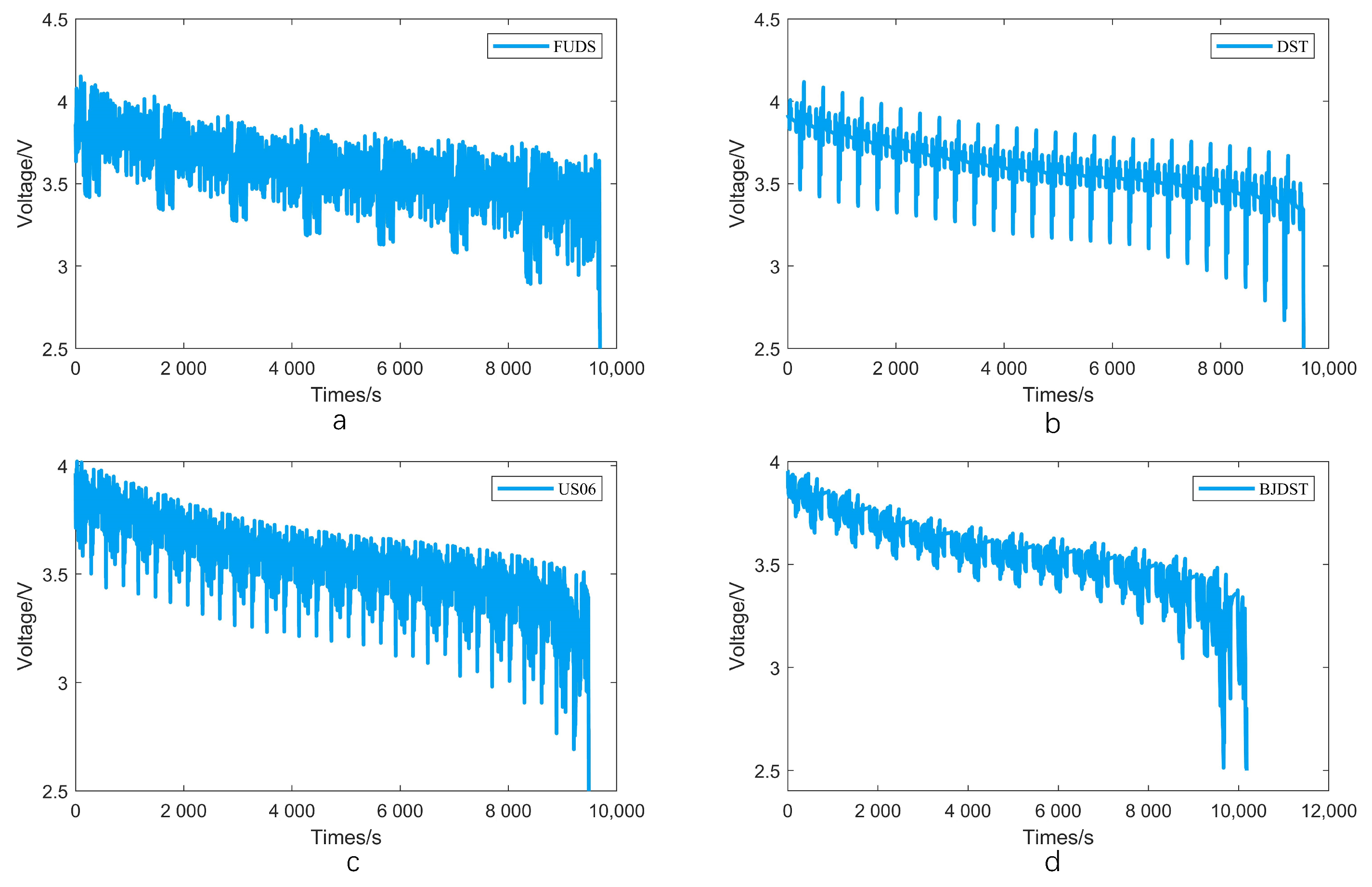
2.1. Experimental Data

Different driving situations, such as city streets and highways, can entail different road conditions for electric vehicles, resulting in power variations when actually using the power cell. Therefore, to study the SOC estimation of electric vehicle power batteries, the discharge mode of the battery needs to be considered first. The experimental data came from the CALCE Center for Advanced Life Cycle Engineering [21]. The battery discharge data in the four working conditions are contained in the Dynamic Stress Test (DST), The Federal Urban Driving Schedule (FUDS), and US06 and Beijing Dynamic Stress Test (BJDST). FUDS is an electric vehicle driving condition proposed in the “USABC Electric Vehicle Experiment Manual” [22], which is used for urban driving conditions. DST is the condition under which the battery is subjected to dynamic stress testing. It is a simplification of the FUDS case. US06 is a type of Federal Test Procedure. It examines the operation of the test vehicle at high speed that is rapidly accelerating. BJDST is based on the working conditions obtained under the Beijing standard dynamic stress test. The current discharge situation of the above working conditions is shown in Figure 1.

The battery in question was a Samsung INR 18650-20R LIB with a rated capacity of 2 Ah to charge or discharge, and it can be monitored at 0° 25° 45°. All data were tested at 80% or 50% SOC. The specific description is that the battery first carried on the constant discharge current for a certain period time, then discharged under working conditions till the electric quantity decreased to a certain percentage.

During the use of an LIB, the disembedding of Li-ions in its interior leads to a decrease in electric charge. The SOC is defined as the ratio of the battery’s remaining capacity compared to the battery’s nominal capacity, which can be expressed by Equation [13]:

$$\mathrm{SOC}=\frac{Q_r}{Q_n}\times 100\%$$

(1)

where Q${}_r$ is the remaining power and Q${}_n$ is the rated capacity of the battery. SOC is an important reference for battery state estimation. It indicates the remaining capacity and how long the battery can be used before it will need to be recharged.

In SOC estimation, as a nonlinear system, its performance is affected by many factors [23,24,25,26]. The three impact factors of current, voltage, and temperature are used in this paper. At low temperatures, the internal chemical reaction rate of the battery becomes slow, resulting in the deterioration of charge and discharge performance [27]. Higher temperatures cause chemical reactions inside the battery to speed up, which can improve charging and discharging performance. The discharge rate of the battery also affects the capacity of the battery [28], the most direct representations of which are the current and voltage. Therefore, we chose real-time current, voltage, and temperature as input features. The trend of voltage change is shown in Figure 2.

2.2. Experimental Model Construction

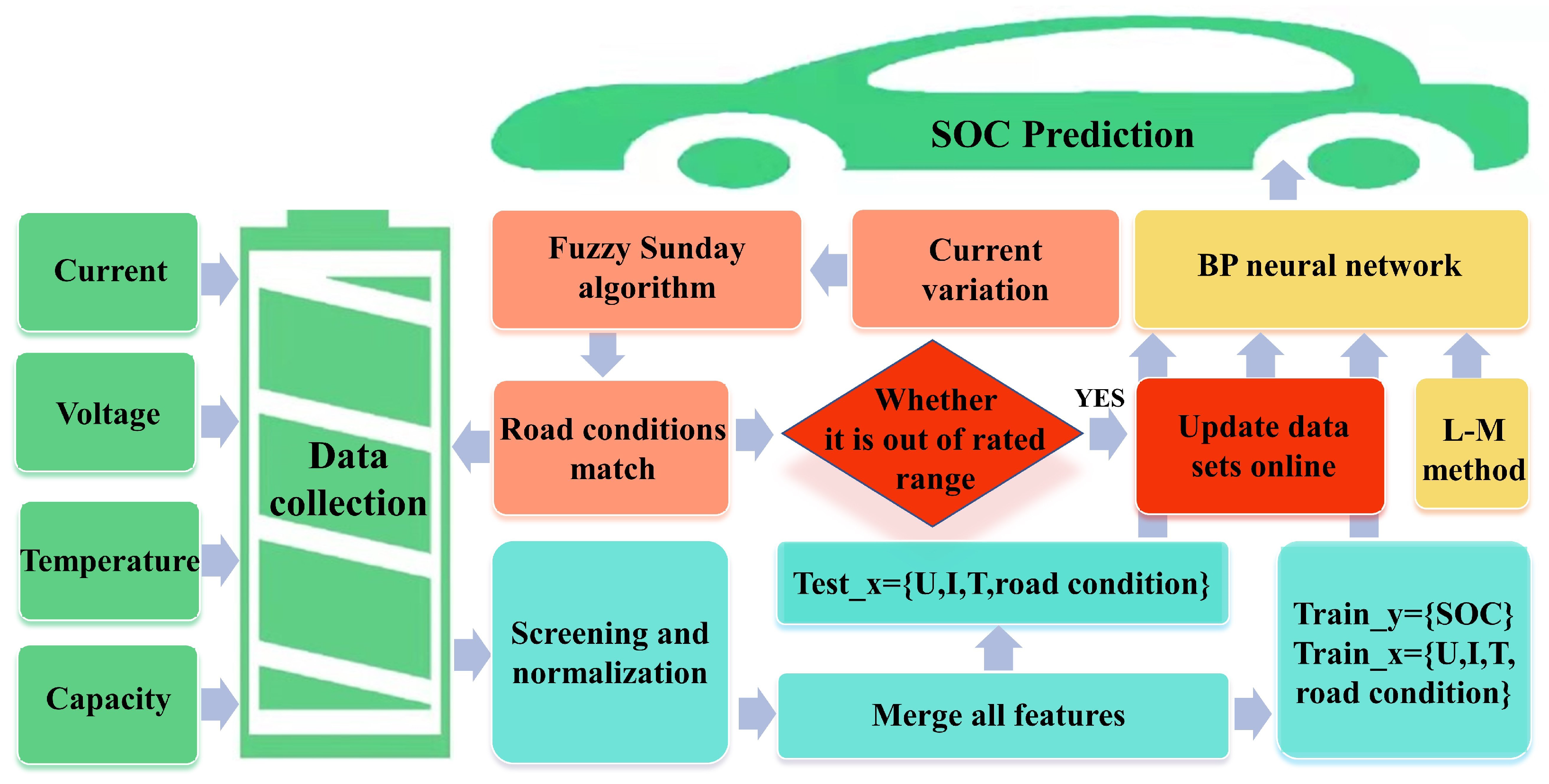
2.2.1. Model Overview

LIBs are affected by external factors and internal chemical structure changes, which means no algorithm can adapt to each estimate of the battery SOC. To make the estimation result as precise as possible, we use the BPNN estimation model based on the fuzzy Sunday algorithm. The model is shown in Figure 3.

Through the analysis in Section 2, real-time current, voltage, and temperature were used during the experiment, and road condition information was added as input features on this basis. Short sequences of current changes are used to match different road conditions. Due to the noise fluctuations in the discharge current of the battery, the current time series cannot be completely matched. This makes pattern matching algorithms unable to collect matching information. Therefore, the Sunday algorithm was improved to obtain road condition information for this phenomenon. After all input features were obtained, data cleaning and normalization were performed to remove abnormal data. We used the BPNN with the L–M method as the training algorithm. It can be seen from the experimental results that the performance is great. When the unknown operating conditions are obtained, the model formulates a special plan for the SOC prediction and analyzes the prediction results.

2.2.2. Improved Fuzzy Sunday Algorithm

The Sunday algorithm is a string matching algorithm proposed by Daniel M. Sunday [29]. When the match fails, the focus is on the last character in the main string that participates in the match. If the character does not appear in the pattern string, skip it directly and move to the last digit of the pattern string; otherwise, move to the corresponding position in the pattern string. In the process of road condition matching, not every discharge current is a fixed value. It has certain fluctuations. The road condition information is not an exact match, so the original Sunday algorithm is not applicable. Therefore, the Sunday algorithm was improved to adapt to road condition information matching. Compared with the traversal method, the Sunday algorithm is highly efficient and responds quickly. The short-term current sequence change was used as a substring in the experiment to perform road condition matching and retrieve the road condition information that it belongs to. However, the change in the current during the driving of a electric vehicle is not an exact number. Its changes are variable and sensitive to external influences. There is no guarantee that the data corresponding to the matching process can be completely matched. Even small gaps can cause matching errors. Based on this requirement, the Sunday algorithm was improved to meet our needs. When the fluctuation of the algorithm did not exceed 2% of the matching data, the corresponding data were considered to match. We modified the corresponding distance in the pattern string that needed to be skipped. If it met the precision requirement of less than 2%, that meant that the substring corresponds to the main string, and then we compared whether the remaining bits were the same, which can be expressed by Algorithm 1.

Algorithm 1 Whether the road conditions match (Sunday).

Ensure:$n\leftarrow length\left[T\right]$ $m\leftarrow length\left[P\right]$ $s\leftarrow 1$ while$s<=n-m+1$do    $j\leftarrow 1$    while $\left|T\right(s+j-1)-P(j\left)\right|<\left(max\right(T)-min(T\left)\right)\ast 2\%$ do      $j\leftarrow j+1$      if $j\ge m+1$ then         $returns$      end if    end while    if a number in the tolerance range of $T(s+m)\pm \left(max\right(T)-min(T\left)\right)\ast 2\%$ in array P then      $shift=find\left(\right|P-T(s+m)|<(max\left(T\right)-min\left(T\right))\ast 2\%)$      $s=s+m-shift\left(end\right)+1$    else      $s=s+m$    end if end while return   $-1$

When the input conditions are unknown, the short-term road condition time series cannot be matched with the road condition information in the database. Reduce the degree of the substring and rematch. When the length is reduced to a certain length, there is still no matching condition, and it is classified as an unknown road condition for prediction. The BPNN is used to ensure prediction accuracy by updating the data in real time. In the process of predicting unknown road conditions, the accuracy of this prediction by the neural network is improved by updating the database in real time.

2.2.3. Backpropagation Neural Network

The training process of BPNN is mainly completed through two stages: forward propagation of signals and backward propagation of errors. If the desired output is not obtained at the output layer, turn to the backpropagation process of the error signal. By alternating these two processes, the error function gradient descent strategy is performed in the weight vector space. Dynamically iteratively searches a set of weight vectors to make the network error function reach the minimum value, thereby completing the process of information extraction and memory [30].

Forward propagation: Let X be the input vector, n be the number of input vectors, Y be the output vector, and m be the number of output vectors, which can be expressed by:

$$\left\{\begin{array}{c}X=\left[\begin{array}{c}{x}_{11},x_{12},\cdots ,x_{1r}\\ x_{21},x_{22},\cdots ,x_{2n}\\ ⋮\\ x_{n1},x_{n2},\cdots ,x_{nr}\end{array}\right]\\ Y={[y_1,y_2,\cdots ,y_m]}^T\end{array}\right.$$

(2)

Calculate the output value of the hidden layer node. Take the hidden layer node i as an example. Set the number of hidden layer nodes to p, set the connection weight of w${}_{1kj}$, the threshold value of node i is b${}_{1j}$, set the input value of a${}_{1j}$, and set the output value of h${}_{1j}$, which can be expressed by the equation:

$$a_{1j}=\sum _{k=1}^n{w}_{1kj}{x}_k,1⩽j⩽p$$

(3)

$$h_j=f(a_{1j}+b_{1j})$$

(4)

where f represents the activation function, and the sigmoid function is used in this paper.

Calculate the output value of the output layer node. Let q be one of the output vectors. The input value is a${}_{2q}$, the output value is O${}_q$, and the threshold is b${}_{2q}$, which can be expressed by:

$$a_{2q}=\sum _{j=1}^m{w}_{2jq}{h}_j,1⩽q⩽m$$

(5)

$$O_m=f(a_{2q}+b_{2q})$$

(6)

Backpropagation: The error signal is entered at the output and then backpropagated through the hidden layer. The error is equally distributed to all units of each layer, and the connection weight of each unit layer is adjusted by the obtained unit signal error of each layer, thereby reducing the error signal. In the process of network operation, the output error of the layer node is calculated and detected, and the error between the output value O${}_q$ and the target value T${}_q$ is $\epsilon$${}_q$, which can be expressed by the equation:

$${\epsilon }_q=\left|O_q-T_q\right|$$

(7)

If the maximum value of the generated errors is less than the allowable error, the training requirement is completed. Otherwise, adjust the network parameters and retrain until all samples meet the conditions. During the backpropagation process, the learning errors of nodes q and j during the training process are defined as d${}_{2q}$ and d${}_{1j}$, which can be expressed by the equation:

$$d_{2q}=O_q(1-O_q)(O_q-T_q)$$

(8)

$$d_{1j}=h_j(1-h_j)\sum _{q=1}^m{w}_{2jq}{d}_{2q}$$

(9)

When the learning error is obtained, the network parameters are adjusted according to their size. Assuming that the weight at time t + 1 is the adjusted weight, the new weight expression equation is as follows:

$$w_{2jq}(t+1)=w_{2jq}\left(t\right)+\eta d_{2q}{h}_j+\alpha [w_{2jq}\left(t\right)-w_{2jq}(t-1)]$$

(10)

$$w_{1kj}(t+1)=w_{1kj}\left(t\right)+\eta d_{1j}{x}_k+\alpha [w_{1kj}\left(t\right)-w_{1kj}(t-1)]$$

(11)

where $\eta$ is the learning rate and $\alpha$ is the momentum factor. The correction threshold b also changes accordingly. The specific change equation is as follows:

$$b_{2q}(t+1)=b_{2q}\left(t\right)+\eta d_{2q}{h}_j+\alpha [b_{2q}\left(t\right)-b_{2q}(t-1)]$$

(12)

$$b_{1j}(t+1)=b_{1j}\left(t\right)+\eta d_{1j}+\alpha [b_{1j}\left(t\right)-b_{1j}(t-1)]$$

(13)

In the experiment, the input features were current, voltage, temperature, and road condition information; and the output was the corresponding SOC value. During network operation, the gradient descent strategy uses the L–M method. L–M is a nonlinear optimization method using the gradient descent method and the Gauss–Newton method [31]. In the running process of the algorithm, it is controlled by the parameters. When there is a certain gap between the parameters and the optimal solution, the gradient descent method is used to update the parameters. When the parameters are close to the optimal value, the Newton method is used to update the parameters [32]. The L–M algorithm can effectively deal with the problem of redundant parameters so that the chance of cost function falling into local minimum is greatly reduced. Therefore, the SOC estimations of a lithium-ion battery in various road conditions are good.

3. Experimental Verification

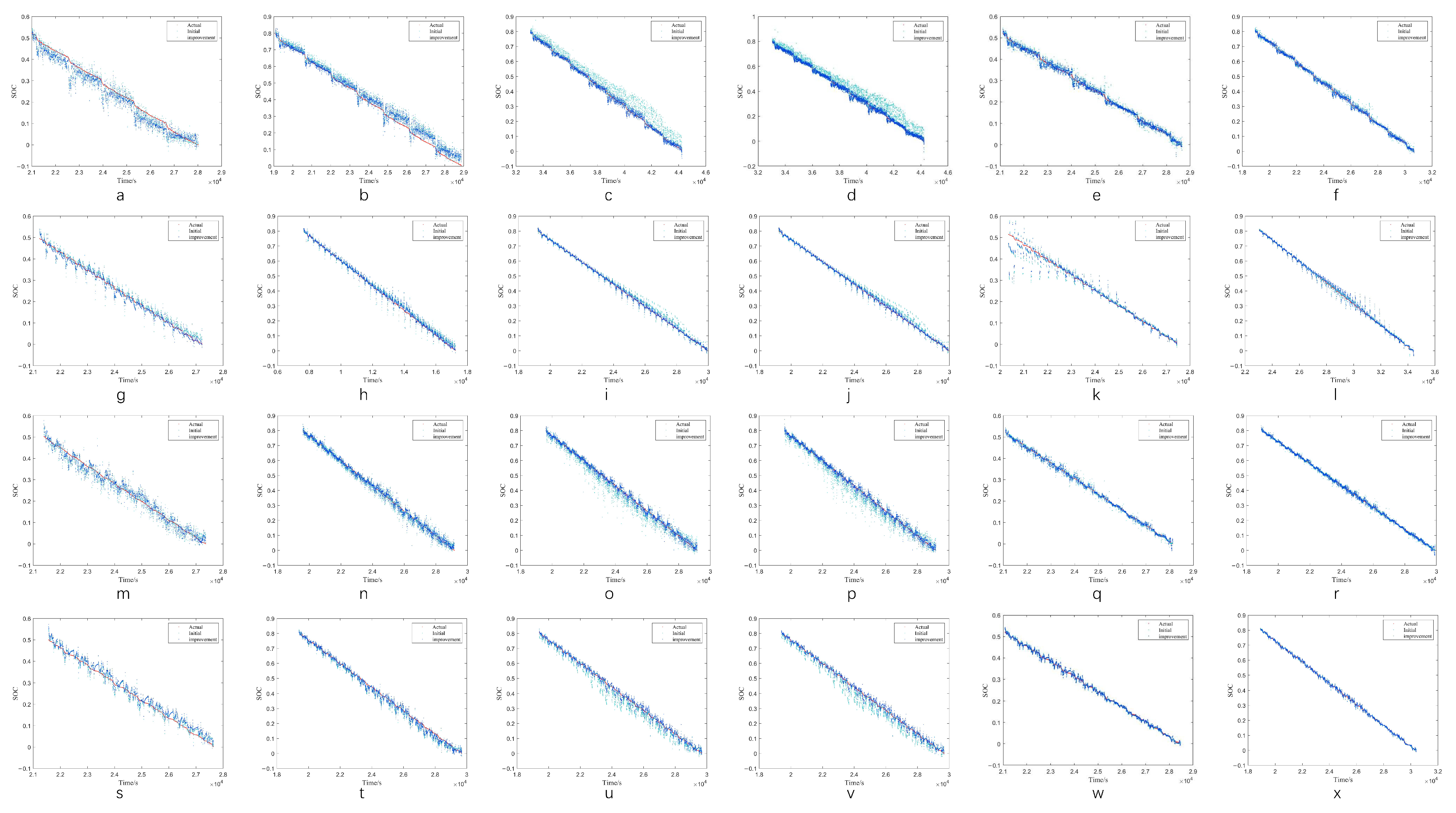
3.1. Experiment and Error Analysis

LIBs with a rated capacity of 2 Ah were selected as the test objects. Training and estimation were performed using twelve batches of discharges under different conditions. To verify whether the prediction results of the features obtained by the improved Sunday matching algorithm were accurate, we used the data with and without road condition information to conduct experiments, as shown in Figure 4. The experimental errors of each group are shown in

Table 1. Estimation error under different working conditions and different temperatures.

Condition	DST
Temperature	0				25				45
State	50		80		50		80		50		80
Improve	No	Yes	No	Yes	No	Yes	No	Yes	No	Yes	No	Yes
MAE	2.60 × 10${}^{-2}$	2.80 × 10${}^{-2}$	2.92 × 10${}^{-2}$	2.48 × 10${}^{-2}$	2.78 × 10${}^{-2}$	9.74 × 10${}^{-3}$	2.79 × 10${}^{-2}$	9.76 × 10${}^{-3}$	8.76 × 10${}^{-3}$	7.37 × 10${}^{-3}$	8.04 × 10${}^{-3}$	7.00 × 10${}^{-3}$
MSE	1.20 × 10${}^{-3}$	1.27 × 10${}^{-3}$	1.31 × 10${}^{-3}$	1.01 × 10${}^{-3}$	1.61 × 10${}^{-3}$	1.72 × 10${}^{-4}$	1.63 × 10${}^{-3}$	1.79 × 10${}^{-4}$	1.56 × 10${}^{-4}$	1.03 × 10${}^{-4}$	1.36 × 10${}^{-4}$	8.68 × 10${}^{-5}$
RMSE	3.35 × 10${}^{-2}$	3.56 × 10${}^{-2}$	3.61 × 10${}^{-2}$	3.17 × 10${}^{-2}$	4.02 × 10${}^{-2}$	1.31 × 10${}^{-2}$	4.04 × 10${}^{-2}$	1.34 × 10${}^{-2}$	1.25 × 10${}^{-2}$	1.01 × 10${}^{-2}$	1.17 × 10${}^{-2}$	9.32 × 10${}^{-3}$
Condition	FUDS
Temperature	0				25				45
State	50		80		50		80		50		80
Improve	No	Yes	No	Yes	No	Yes	No	Yes	No	Yes	No	Yes
MAE	1.42 × 10${}^{-2}$	1.17 × 10${}^{-2}$	1.37 × 10${}^{-2}$	8.93 × 10${}^{-3}$	1.20 × 10${}^{-2}$	5.02 × 10${}^{-3}$	1.22 × 10${}^{-2}$	5.06 × 10${}^{-3}$	1.51 × 10${}^{-2}$	1.20 × 10${}^{-2}$	5.80 × 10${}^{-3}$	7.67 × 10${}^{-3}$
MSE	3.59 × 10${}^{-4}$	2.54 × 10${}^{-4}$	3.63 × 10${}^{-4}$	1.88 × 10${}^{-4}$	3.08 × 10${}^{-4}$	5.56 × 10${}^{-5}$	3.20 × 10${}^{-4}$	5.68 × 10${}^{-5}$	9.12 × 10${}^{-4}$	6.41 × 10${}^{-4}$	9.01 × 10${}^{-5}$	1.78 × 10${}^{-4}$
RMSE	1.89 × 10${}^{-2}$	1.60 × 10${}^{-2}$	1.91 × 10${}^{-2}$	1.37 × 10${}^{-2}$	1.76 × 10${}^{-2}$	7.46 × 10${}^{-3}$	1.79 × 10${}^{-2}$	7.54 × 10${}^{-3}$	3.02 × 10${}^{-2}$	2.53 × 10${}^{-2}$	9.50 × 10${}^{-3}$	1.34 × 10${}^{-2}$
Condition	US06
Temperature	0				25				45
State	50		80		50		80		50		80
Improve	No	Yes	No	Yes	No	Yes	No	Yes	No	Yes	No	Yes
MAE	1.93 × 10${}^{-2}$	1.81 × 10${}^{-2}$	1.53 × 10${}^{-2}$	1.27 × 10${}^{-2}$	2.56 × 10${}^{-2}$	1.28 × 10${}^{-2}$	2.65 × 10${}^{-2}$	1.27 × 10${}^{-2}$	6.74 × 10${}^{-3}$	6.00 × 10${}^{-3}$	5.97 × 10${}^{-3}$	5.29 × 10${}^{-3}$
MSE	6.31 × 10${}^{-4}$	5.28 × 10${}^{-4}$	4.30 × 10${}^{-4}$	2.99 × 10${}^{-4}$	1.30 × 10${}^{-3}$	2.93 × 10${}^{-4}$	1.43 × 10${}^{-3}$	2.91 × 10${}^{-4}$	9.37 × 10${}^{-5}$	6.13 × 10${}^{-5}$	7.54 × 10${}^{-5}$	4.93 × 10${}^{-5}$
RMSE	2.51 × 10${}^{-2}$	2.30 × 10${}^{-2}$	2.07 × 10${}^{-2}$	1.73 × 10${}^{-2}$	3.61 × 10${}^{-2}$	1.71 × 10${}^{-2}$	3.78 × 10${}^{-2}$	1.71 × 10${}^{-2}$	9.68 × 10${}^{-3}$	7.83 × 10${}^{-3}$	8.68 × 10${}^{-3}$	7.02 × 10${}^{-3}$
Condition	BJDST
Temperature	0				25				45
State	50		80		50		80		50		80
Improve	No	Yes	No	Yes	No	Yes	No	Yes	No	Yes	No	Yes
MAE	1.66 × 10${}^{-2}$	1.86 × 10${}^{-2}$	1.74 × 10${}^{-2}$	1.30 × 10${}^{-2}$	2.49 × 10${}^{-2}$	1.11 × 10${}^{-2}$	2.55 × 10${}^{-2}$	1.12 × 10${}^{-2}$	5.00 × 10${}^{-3}$	5.02 × 10${}^{-3}$	4.53 × 10${}^{-3}$	4.69 × 10${}^{-3}$
MSE	4.04 × 10${}^{-4}$	4.90 × 10${}^{-4}$	5.34 × 10${}^{-4}$	3.16 × 10${}^{-4}$	1.23 × 10${}^{-3}$	2.32 × 10${}^{-4}$	1.29 × 10${}^{-3}$	2.29 × 10${}^{-4}$	4.41 × 10${}^{-5}$	4.37 × 10${}^{-5}$	3.58 × 10${}^{-5}$	3.76 × 10${}^{-5}$
RMSE	2.01 × 10${}^{-2}$	2.21 × 10${}^{-2}$	2.31 × 10${}^{-2}$	1.78 × 10${}^{-2}$	3.51 × 10${}^{-2}$	1.52 × 10${}^{-2}$	3.60 × 10${}^{-2}$	1.51 × 10${}^{-2}$	6.64 × 10${}^{-3}$	6.61 × 10${}^{-3}$	5.98 × 10${}^{-3}$	6.13 × 10${}^{-3}$

. The results of SOC estimation with or without road condition information are shown in the table. Estimates were made at different temperatures and under different road conditions. Among the 24 sets of test results, 20 sets had reduced errors after application of the improved algorithm. The experimental results show that the model can accurately estimate the SOC under different temperatures and different road conditions, indicating that the model has good adaptability.

Although the prediction results of the BPNN without the use of road condition information were relatively satisfactory, the predictions were greatly improved after adding it. It can be seen in the figure and table that in most cases, the predictions after adding road condition features were more accurate. We can say that the predictions of the road condition information obtained by the Sunday algorithm were accurate, as shown in

Table 2. Error summary.

Improve	No			Yes
Error	MAE	MSE	RMSE	MAE	MSE	RMSE
Summary	1.65 × 10${}^{-2}$	6.73 × 10${}^{-4}$	2.59 × 10${}^{-2}$	1.07 × 10${}^{-2}$	2.70 × 10${}^{-4}$	1.64 × 10${}^{-2}$
FUDS	2.14 × 10${}^{-2}$	3.60 × 10${}^{-4}$	3.19 × 10${}^{-2}$	1.37 × 10${}^{-2}$	2.01 × 10${}^{-4}$	2.05 × 10${}^{-2}$
DST	1.17 × 10${}^{-2}$	3.60 × 10${}^{-4}$	1.90 × 10${}^{-2}$	7.84 × 10${}^{-3}$	2.01 × 10${}^{-4}$	1.42 × 10${}^{-2}$
US06	1.65 × 10${}^{-2}$	6.69 × 10${}^{-4}$	2.59 × 10${}^{-2}$	1.09 × 10${}^{-2}$	2.38 × 10${}^{-4}$	1.54 × 10${}^{-2}$
BJDST	1.59 × 10${}^{-2}$	6.25 × 10${}^{-4}$	2.50 × 10${}^{-2}$	1.02 × 10${}^{-2}$	2.10 × 10${}^{-4}$	1.45 × 10${}^{-2}$

, which is a summary error picture. In Table 2, it can be seen that the errors were greatly reduced after the use of road condition information.

For the SOC estimations without road condition information: MAE was 1.65 × 10${}^{-2}$, MSE was 6.73 × 10${}^{-4}$, and RMSE was 2.59 × 10${}^{-2}$. After adding road condition information: MAE was 1.07 × 10${}^{-2}$, MSE was 2.70 × 10${}^{-4}$, and RMSE was 1.64 × 10${}^{-2}$. The error evaluation indicators decreased by 35.15%, 59.89%, and 36.68%. Whether we talk of the estimation of different road conditions or the estimation of SOC, the accuracy was significantly improved.

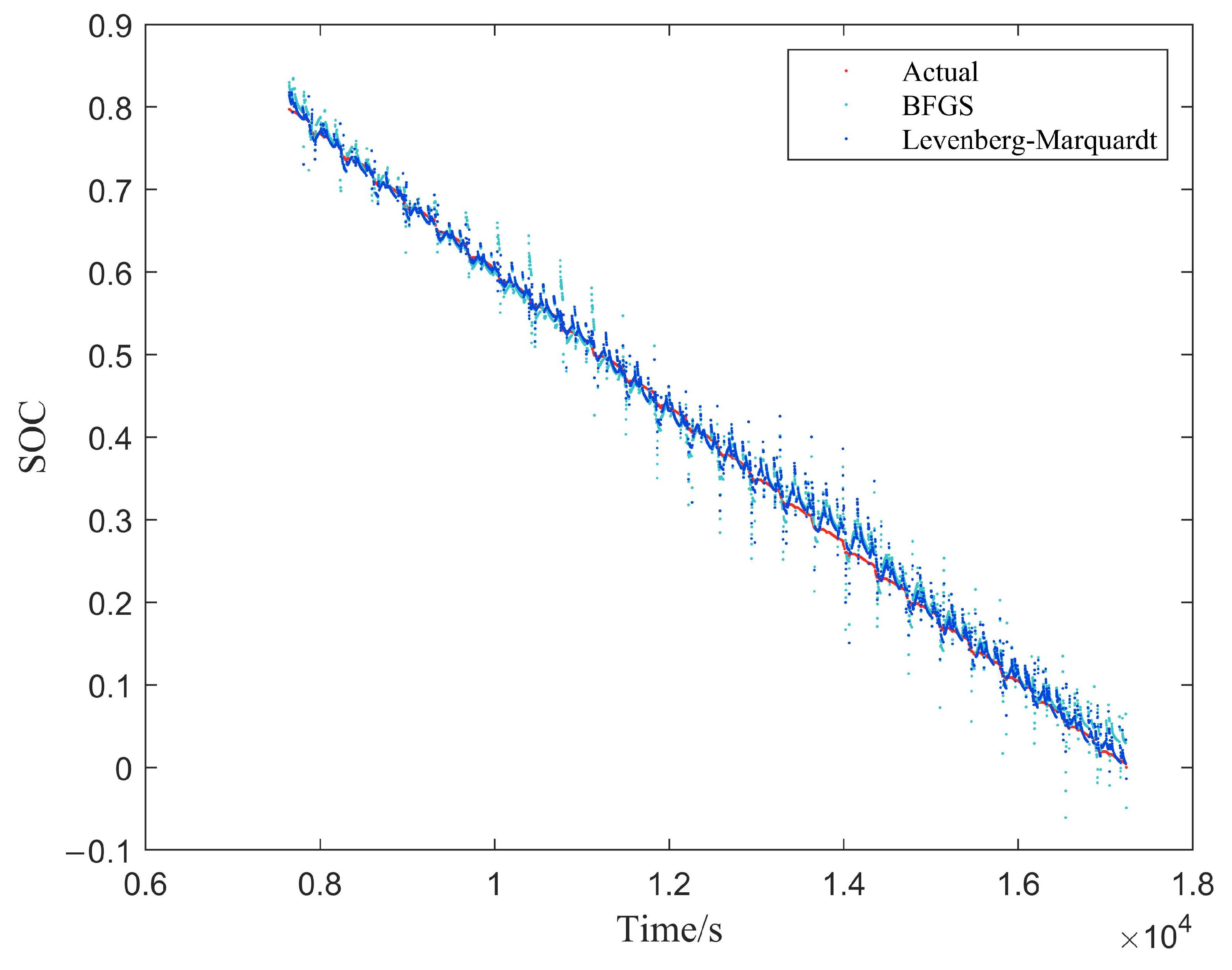
3.2. Analysis of the Training Algorithm

To prove the superiority and objectivity of the algorithm, the training algorithm of the BPNN was modified in the experiment to obtain optimal performance. Compared to the quasi-Newton method (BFGS), it can be seen that the L–M training algorithm has better convergence. The comparison results show that the estimation results of the L–M method have the smallest error rate: MAE was 1.07 × 10${}^{-2}$, MSE was 2.70 × 10${}^{-4}$, and RMSE was 1.64 × 10${}^{-2}$. The reason is that the L–M algorithm combines the advantages of the gradient descent method and the Newton method. The damping coefficient is added to the algorithm to control the iterative step size and direction of each step so that the algorithm converges faster. In the actual process, the L–M algorithm can effectively deal with redundant information, and when it is used for SOC estimation, it can handle the data of different road conditions very well, making the estimates more ideal. Taking DST road conditions, the temperature of 0°, and 80% SOC estimation as an example, as shown in Figure 5, the overall error analysis is shown in

Table 3. Training algorithms error.

Method	L–M	BFGS
MAE	1.07 × 10${}^{-2}$	1.40 × 10${}^{-2}$
MSE	2.70 × 10${}^{-4}$	3.84 × 10${}^{-4}$
RMSE	1.64 × 10${}^{-2}$	1.96 × 10${}^{-2}$

.

4. Discussion

4.1. Estimation Strategies for Unknown Road Conditions

According to our analysis of the above estimation results, the model can obtain accurate SOC estimates when the road condition information is known. If an electric vehicle enters an unknown area, can a more accurate estimation result be obtained? During the experiment, we did not improve the original model and directly estimated the SOC in unknown road conditions. The MAE was 2.19 × 10${}^{-1}$, the MSE was 5.08 × 10${}^{-2}$, and the RMSE was 2.58 × 10${}^{-1}$. It can be seen that the obtained estimates were not ideal. To make the overall model more perfect, we need to improve the accuracy of the model when the road conditions are unknown. An analysis was performed for the event of the predictions being made after loading the data of the unknown operating conditions. We reduced the substring size and matched again if the match failed when loading an unknown cause. However, that way, it is still possible that the corresponding road conditions cannot be matched. For the data loaded with unknown working conditions, we used the method of continuously updating the dataset to improve its accuracy, and the prediction effect can also be stabilized in an ideal state by updating the dataset. At this point, we have to consider the time consumption of the algorithm. Due to the large dataset, the network needs to be retrained for each update, which is very expensive. We used random sampling, extracting one hundred data from the database each time, plus the updated data under DST road conditions for training, and then performed online prediction. The prediction effect was better: MAE was 1.19 × 10${}^{-2}$, MSE was 4.00 × 10${}^{-4}$, and RMSE was 2.00 × 10${}^{-2}$. The time overhead was large. The shortest time was 0.5 s, and the longest time was 4.8 s. Compared with no database update, this strategy has a larger time overhead, but it meets the accuracy requirements. The direct training and prediction method without any changes is very ineffective. The reason is that there are no corresponding data in the training set for these road conditions, so unknown features appear in the prediction process, resulting in unsatisfactory results. The specific need is to remove the DST-related data from the database, and then use it as an unknown operating condition for battery state-of-charge estimation. The prediction results of using three different schemes—adding road condition information, not adding road condition information, and adding road condition information in real time to update the database—are compared for DST road conditions, temperature 0°, and 80% SOC in Figure 6, and the specific error analysis is shown in

Table 4. Estimation error analysis of unknown road information with different strategies.

Method	Add	Not Added	Add and Update
MAE	2.19 × 10${}^{-1}$	2.32 × 10${}^{-2}$	1.19 × 10${}^{-2}$
MSE	5.08 × 10${}^{-2}$	1.15 × 10${}^{-3}$	4.00 × 10${}^{-4}$
RMSE	2.58 × 10${}^{-1}$	3.40 × 10${}^{-2}$	2.00 × 10${}^{-2}$
Time consuming/s	0.197	0.086	0.516

. Therefore, the improved strategy proposed for unknown road width significantly improved the estimation accuracy for the SOC. Error was reduced by an order of magnitude, in fact.

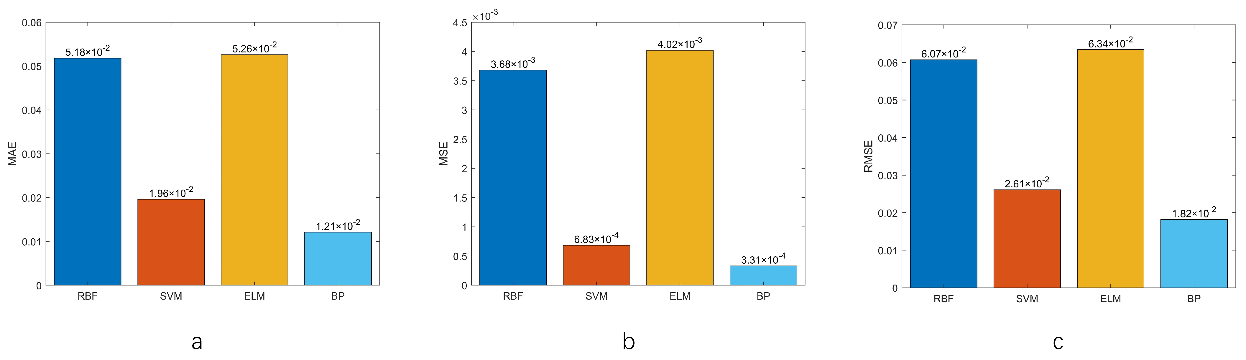
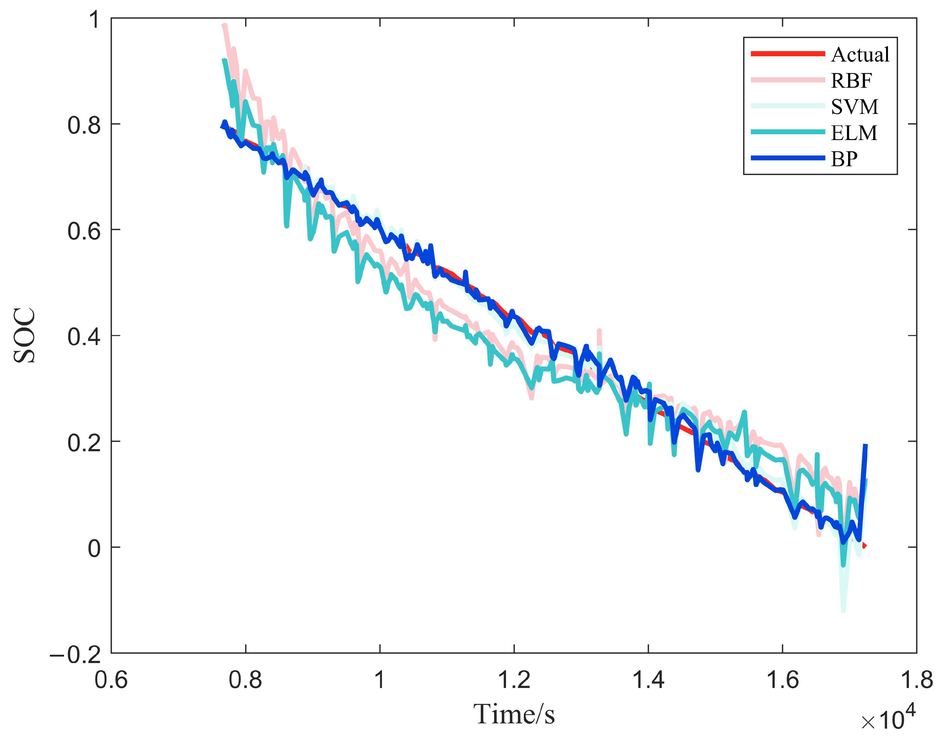
4.2. Comparison with Other SOC Models

Through the above experiments, a complete and accurate SOC estimation model was obtained, but it needed to be compared with other related prediction models. This section compares our model with four predictive models. The experimental process involved sampling experiments, extracting 10,000 data nodes from all data for training, and extracting 5000 data nodes for verification. The experiment compared not only the error of the results but also the time taken. For DST road conditions, the temperature at 0°, and 80% SOC as an example, see Figure 7 and

Table 5. The comparison of algorithms’ error.

Algorithm	RBF	SVM	ELM	BP
MAE	5.18 × 10${}^{-2}$	1.96 × 10${}^{-2}$	5.26 × 10${}^{-2}$	1.21 × 10${}^{-2}$
MSE	3.68 × 10${}^{-3}$	6.83 × 10${}^{-4}$	4.02 × 10${}^{-3}$	3.31 × 10${}^{-4}$
RMSE	6.07 × 10${}^{-2}$	2.61 × 10${}^{-2}$	6.34 × 10${}^{-2}$	1.82 × 10${}^{-2}$
Time consuming/s	6.241	2.378	0.006	0.173

. To visually compare the error of each algorithm, see Figure 8.

It can be seen in the table that the error of the support vector machine was the smallest among the four prediction algorithms: radial basis function network (RBF), support vector machine (SVM), extreme learning machine (ELM), and BPNN. The RBF network differs from BPNN in its activation function, and it does not calculate model parameters with the backpropagation algorithm. Although the RBF neural network has a good nonlinear fitting ability, its network is more complex. When there are more training samples, the number of hidden layer neurons of the RBF neural network is much higher than that of BPNN, which means that the time cost will increase to some extent. Due to the complexity of battery chemical reactions in SOC estimation, the parameters used are not comprehensive. Therefore, a strong mapping relationship may not be able to obtain a more accurate estimate. The support vector machine is a learning method that uses structural risk minimization criteria. With a large number of databases with different road conditions, the error obtained by SVM still cannot reach the desired effect. In addition, with an increase in data volume, its time cost continues to increase, which is not conducive to our real-time prediction. The hidden layer of the extreme learning machine requires no iteration and learns quickly. However, it does not take into account the structural risk, so overfitting may arise. Additionally, the performance of the model will be greatly affected when the data have outliers. The ELM has the shortest running time; it only took 0.006 s to make predictions, but the error was too large. Therefore, BPNN is the optimal choice, as it can obtain the most accurate prediction results within a short time.

5. Conclusions

With the development of SOC estimation methods, the improvements in model accuracy are accompanied by longer running times. In order to ensure real-time updating of SOC estimates and how to accurately estimate SOC with different road condition information, we propose a method of state estimation based on the fuzzy Sunday algorithm. It analyzes the battery-power-related characteristic data and maps the results to the characteristic node. A Sunday algorithm is used to gather road condition information, which is ignored in other algorithms. The acquired road condition information, and current, voltage, and temperature, are used as model training features. This method improves the anti-interference ability, accuracy, and timeliness of the whole prediction model. In the experiments, the SOC under different temperature and road conditions was estimated, which showed that the model can accurately estimate SOC in various scenarios. By comparing various training algorithms with BPNN, a better scheme was obtained. The SOC estimation strategy for unknown road conditions also enables the model to take into account the response speed on the premise of ensuring the estimation accuracy. Finally, the results of our experimental model were compared with those of RBF, SVM, and ELM. By comparing several evaluation indexes, this method can help users to monitor SOC in real time and provides the system with high sensitivity. Accurate SOC estimates also reduce travel anxiety for users. The results showed that the model is an effective battery evaluation method.

References

1. Stampatori, D.; Raimondi, P.P.; Noussan, M. Li-ion batteries: A review of a key technology for transport decarbonization. Energies 2020, 13, 2638. [Google Scholar] [CrossRef]
2. Yu, W.; Chao, W.; Xingsheng, G. Research on fault diagnosis method for over-discharge of power lithium battery. In Theory, Methodology, Tools and Applications for Modeling and Simulation of Complex Systems; Springer: Singapore, 2016; pp. 308–314. [Google Scholar]
3. Huang, B.; Pan, Z.; Su, X.; An, L. Recycling of lithium-ion batteries: Recent advances and perspectives. J. Power Sources 2018, 399, 274–286. [Google Scholar] [CrossRef]
4. Hu, X.; Feng, F.; Liu, K.; Zhang, L.; Xie, J.; Liu, B. State estimation for advanced battery management: Key challenges and future trends. Renew. Sustain. Energy Rev. 2019, 114, 109334. [Google Scholar] [CrossRef]
5. Ng, K.S.; Moo, C.; Chen, Y.; Hsieh, Y. Enhanced coulomb counting method for estimating state-of-charge and state-of-health of lithium-ion batteries. Appl. Energy 2009, 86, 1506–1511. [Google Scholar] [CrossRef]
6. Weng, C.; Sun, J.; Peng, H. A unified open-circuit-voltage model of lithium-ion batteries for state-of-charge estimation and state-of-health monitoring. J. Power Sources 2014, 258, 228–237. [Google Scholar] [CrossRef]
7. He, Z.; Yang, Z.; Cui, X.; Li, E. A method of state-of-charge estimation for EV power lithium-ion battery using a novel adaptive extended kalman filter. IEEE Trans. Veh. Technol. 2020, 69, 14618–14630. [Google Scholar] [CrossRef]
8. Sun, D.; Yu, X.; Zhang, C.; Wang, C.; Huang, R. State of charge estimation for lithium-ion battery based on an intelligent adaptive unscented Kalman filter. Int. J. Energy Res. 2020, 44, 11199–11218. [Google Scholar] [CrossRef]
9. Lai, X.; Yi, W.; Zheng, Y.; Zhou, L. An all-region state-of-charge estimator based on global particle swarm optimization and improved extended kalman filter for lithium-ion batteries. Electronics 2018, 7, 321. [Google Scholar] [CrossRef] [Green Version]
10. Ye, M.; Guo, H.; Cao, B. A model-based adaptive state of charge estimator for a lithium-ion battery using an improved adaptive particle filter. Appl. Energy 2017, 190, 740–748. [Google Scholar] [CrossRef]
11. Lipu, H.; Hannan, M.A.; Hussain, A.; Ayob, A.; Saad, M.H.; Muttaqi, K.M. State of charge estimation in lithium-ion batteries: A neural network optimization approach. Electronics 2020, 9, 1546. [Google Scholar] [CrossRef]
12. Rivera-Barrera, J.P.; Muñoz-Galeano, N.; Sarmiento-Maldonado, H.O. SoC Estimation for Lithium-ion Batteries: Review and Future Challenges. Electronics 2017, 6, 102. [Google Scholar] [CrossRef] [Green Version]
13. Cheng, A.; Wang, Y. A Novel State of Charge Estimation Method of Batteries Using Recurrent Neural Networks. In Proceedings of the 2018 International Conference on Network, Communication, Computer Engineering (NCCE 2018), Chongqing, China, 26–27 May 2018. [Google Scholar]
14. Liu, Z.; Dang, X.; Jing, B.; Ji, J. A novel model-based state of charge estimation for lithium-ion battery using adaptive robust iterative cubature kalman filter. Electr. Power Syst. Res. 2017, 177, 105951. [Google Scholar] [CrossRef]
15. Chen, X.; Chen, X.; Chen, X. A novel framework for lithium-ion battery state of charge estimation based on Kalman filter Gaussian process regression. Int. J. Energy Res. 2021, 45, 13238–13249. [Google Scholar] [CrossRef]
16. Xie, F. A novel battery state of charge estimation based on the joint unscented kalman filter and support vector machine algorithms. Electr. Power Syst. Res. 2020, 8, 7935–7953. [Google Scholar] [CrossRef]
17. Wang, C.; Fan, X.; Zhang, X.; Gao, L.; Liu, H. An evaluation method of li-ion batteries state of charge based on irvm and verified by simulation. Appl. Electron. Tech. 2018, 44, 127–130. [Google Scholar]
18. Wan, X.; Yang, B.; Fan, Z. Improved Sunday Pattern Matching Algorithm. Appl. Electron. Tech. 2009, 35, 125–126. [Google Scholar]
19. Alicherry, M.; Muthuprasanna, M.; Kumar, V. High Speed Pattern Matching for Network IDS/IPS. In Proceedings of the 2006 IEEE International Conference on Network Protocols, Santa Barbara, CA, USA, 12–15 November 2006; pp. 187–196. [Google Scholar]
20. Baeza-Yates, R.; Gonnet, G.H. A New Approach to Text Searching. Commun. ACM 1992, 35, 74–82. [Google Scholar] [CrossRef]
21. He, W.; Williard, N.; Chen, C.; Pecht, M. State of charge estimation for li-ion batteries using neural network modeling and unscented kalman filter-based error cancellation. Int. J. Electr. Power Energy Syst. 2014, 62, 783–791. [Google Scholar] [CrossRef]
22. Hunt, G. Usabc Electric Vehicle Battery Test Procedures Manual; Office of Scientific & Technical Information Technical Reports; United States Department of Energy: Washington, DC, USA, 1996.
23. Jiang, F.; Yang, J.; Cheng, Y.; Zhang, X.; Yang, Y.; Gao, K.; Peng, J.; Huang, Z. An aging-aware soc estimation method for lithium-ion batteries using xgboost algorithm. In Proceedings of the 2019 IEEE International Conference on Prognostics and Health Management (ICPHM), San Francisco, CA, USA, 17–20 June 2019. [Google Scholar]
24. Song, S.; Zhang, X.; Gao, D.; Jiang, F.; Wu, Y.; Huang, J.; Gong, Y.; Liu, B.; Huang, Z. A hierarchical state of charge estimation method for lithium-ion batteries via xgboost and kalman filter. In Proceedings of the 2020 IEEE International Conference on Systems, Man, and Cybernetics (SMC), Toronto, ON, Canada, 11–14 October 2020. [Google Scholar]
25. Al-Gabalawy, M.; Hosny, N.S.; Dawson, J.A.; Omar, A.I. State of charge estimation of a li-ion battery based on extended kalman filtering and sensor bias. Int. J. Energy Res. 2021, 45, 6708–6726. [Google Scholar] [CrossRef]
26. Tian, J.; Xiong, R.; Shen, W.; Lu, J. State-of-charge estimation of lifepo4 batteries in electric vehicles: A deep-learning enabled approach. Appl. Energy 2021, 291, 116812. [Google Scholar] [CrossRef]
27. Ma, S.; Jiang, M.; Tao, P.; Song, C.; Wu, J.; Wang, J.; Shang, W. Temperature effect and thermal impact in lithium-ion batteries: A review. Prog. Nat. Sci. Mater. Int. 2018, 28, 653–666. [Google Scholar] [CrossRef]
28. Qin, Y.; Adams, S.; Yuen, C. Transfer learning-based state of charge estimation for lithium-ion battery at varying ambient temperatures. IEEE Trans. Ind. Inform. 2021, 17, 7304–7315. [Google Scholar] [CrossRef]
29. Sunday, D.M. A very fast substring search algorithm. Commun. ACM 1990, 33, 132–142. [Google Scholar] [CrossRef]
30. Yufang, F.; Houqing, L.; Hong, Y. Study on fault diagnosis model based on bp neural network. Comput. Eng. Appl. 2019, 55, 24–30. [Google Scholar]
31. Marquardt, D.W. An algorithm for least-squares estimation of non-linear parameters. J. Soc. Ind. Appl. Math. 1963, 11, 431–441. [Google Scholar] [CrossRef]
32. Gavin, H.P. The Levenberg–Marquardt Algorithm for Nonlinear Least Squares Curve-Fitting Problems; Department of Civil and Environmental Engineering, Duke University: Duke, NC, USA, 2019; Volume 19. [Google Scholar]
Figure 1. Current changes under different working conditions. (a) The diagram of current and time under FUDS conditions. (b) The diagram of current and time under DST conditions. (c) The diagram of current and time under US06 conditions. (d) The diagram of current and time under BJDST conditions.
Energies 15 02853 g001
Figure 2. Current changes under different working conditions. (a) The diagram of voltage and time change under FUDS conditions. (b) The diagram of voltage and time change under DST conditions. (c) The diagram of voltage and time change under US06 conditions. (d) The diagram of voltage and time change under BJDST conditions.
Energies 15 02853 g002
Figure 3. Charge state estimation model based on fuzzy Sunday algorithm.
Energies 15 02853 g003
Figure 4. Estimations of SOC with road condition information. (af) The SOC estimates when SOC was 50% or 80% under the FUDS operating condition of 0°, 25°, or 45°. (gl) The SOC estimates under DST conditions. (mr) The SOC estimates under US06 conditions. (sx) The SOC estimates under BJDST conditions.
Energies 15 02853 g004
Figure 5. Estimated results of different training algorithms.
Energies 15 02853 g005
Figure 6. Estimation of unknown road conditions.
Energies 15 02853 g006
Figure 7. The comparison of algorithms’ estimates.
Energies 15 02853 g007
Figure 8. Comparison algorithms error analysis. (a) MAE. (b) MSE. (c) RMSE.
Energies 15 02853 g008