The Structure of Permafrost in Northern West Siberia: Geophysical Evidence

Abstract

The permafrost of Arctic West Siberia stores extremely rich resources of hydrocarbon fuels that remain a key energy source and an important element of the global economy. A large amount of natural gas in permafrost is bound in gas hydrates which may become an alternative fuel of the future. Shallow subsurface in the permafrost area of northern West Siberia has been studied by transient electromagnetic (TEM) soundings to estimate the permafrost thickness and to detect faults as channels for fluids and heaving features as possible indicators of gas hydrate accumulations. The shallow transient electromagnetic (sTEM) surveys were conducted in discontinuous and continuous permafrost at two sites in northern West Siberia (the northeastern Yamal Peninsula and the southern Gydan Peninsula), with a focus on the vicinities of lakes and cryogenic landforms (frost mounds). The sTEM method resolves well the heterogeneous permafrost structure, with faults, numerous unfrozen zones (taliks), and frost mounds marked by resistivity and seismic anomalies. Some lakes are located above faults, and their origin may be related to deformation, whereas the frost mounds may mark deep-seated fluid dynamic processes. Local thickening of permafrost may be associated with the presence of gas hydrates. The detected features may trace gas migration pathways and reveal possible sites of gas emission.

1. Introduction

The permafrost of northern West Siberia stores extremely rich resources of hydrocarbon fuels that remain a key source of energy and an essential element in the global economy. A large amount of natural gas in permafrost exists in the clathrate form. Gas hydrates may become an important fuel in the future and an alternative to conventional oil and gas energy sources. In this respect, exploration for permafrost gas hydrates has been a new trend of geophysical surveys in the Arctic part of the West Siberian basin. The permafrost structure is another key target of surveys, as it can provide evidence of tectonic and fluid-dynamic processes as the main controls of the distribution and migration paths of hydrocarbons.

Permafrost in northern West Siberia has a complicated structure, with unfrozen zones (taliks), lenses of saline water (cryopegs), and frost heaving features (mounds). However, the permafrost structure has been changing lately under increasing anthropogenic loads associated with drilling and the creation of infrastructure for petroleum production and transportation, which interfere with the natural temperature patterns.

Imaging the permafrost is critical for monitoring its thermal state, with implications for global warming and petroleum exploration issues. On the other hand, exploration in permafrost requires special care to minimize risks of infrastructure damage and improve operation safety. While imaging the permafrost structure, geophysical surveys can help predict potential events of explosive gas emission from beneath frost heaves.

Various geophysical methods were carried out for permafrost studies within Western Siberia.

However, the presence of frozen rocks in the geological section and the high variability of their properties form a number of obstacles in geophysical surveying:

• For Ground-penetrating radar (GPR), the investigation depth is limited to 2–5 m, which does not allow mapping the permafrost base, which can bed on the depth of 500 m in the observed geological settings.
• Direct current (DC) methods application is limited due to the screening effect of highly resistive frozen rocks.
• DC methods are applicable only in the summer season due to the necessity of maintaining the grounding of electrodes.

The transient electromagnetic method in the near field zone (TEM) has certain advantages when applied in Western Siberia and has been proven with numerous scientific research [1,2,3,4,5,6,7,8].

In the Russian Arctic, the TEM method has practically not been applied for permafrost studies. However, to date, TEM surveys are being carried out in vast areas—thousands of square kilometers [9].

The thickness of the permafrost within Western Siberia reaches 500 m. However, nowadays, most geophysical studies are carried out at shallow depths—up to 10–50 m, when investigation depth is limited to 100 m. Rare thermometric wells most often do not reach the depth of 100 m. In most cases, there is no stratigraphy down to a depth of 500 m in deep wells.

TEM surveys are applicable to study the permafrost to a depth of 500 m or even deeper.

The TEM data were analyzed in situ with a lack of drilling data (lithology, stratigraphy, logging, thermometry), but this made it possible to obtain not only a geological and geophysical model of the cryolithozone corresponding to the general ideas of the structure of the region [10,11] but also detailed the internal structure of the cryolithozone (layers permafrost, taliks, cryopegs, gas hydrate deposits, gas migration channels).

Shallow transient electromagnetic (sTEM), with penetration up to 500 m, has been progressively becoming more widely used in permafrost areas due to high sensitivity of differentiation between frozen and unfrozen rocks. TEM responses of frozen earth can be used to contour the extent of permafrost and to estimate its thickness. The method can determine the type of permafrost (continuous, discontinuous, sporadic) and resolve such features as taliks and gas migration pathways.

2. Study Area and Methods

2.1. Study Area

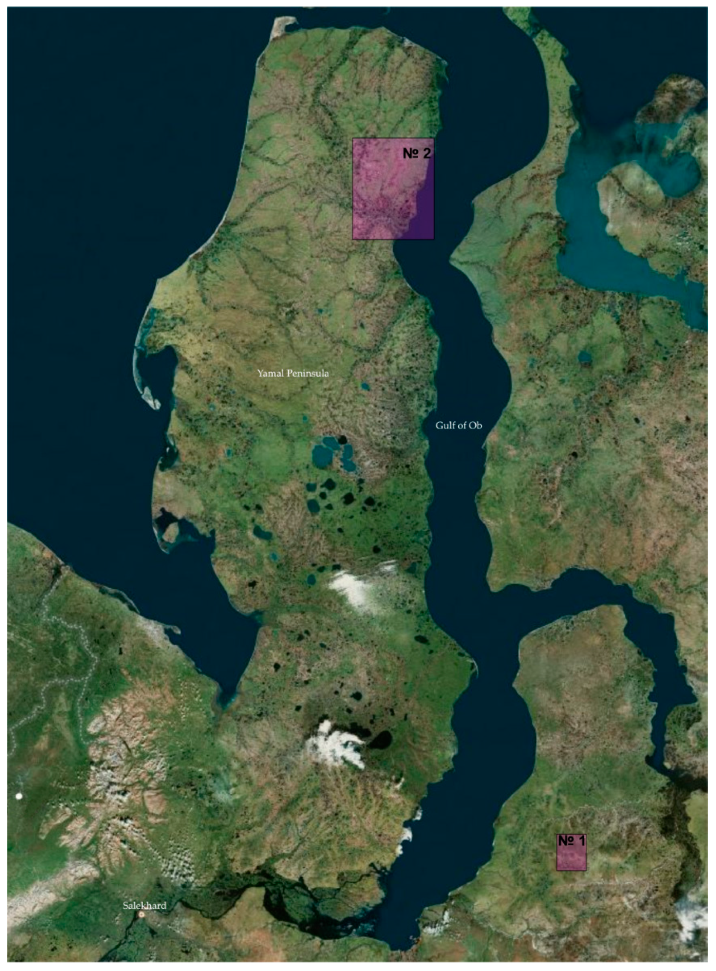
Shallow transient electromagnetic (sTEM) surveys were conducted in two sites of continuous and discontinuous permafrost within oil and gas fields, up to a depth of 500 m (Figure 1).

Site 1 is located in the Nadym-Pur interfluve of the West Siberian basin (southern Gydan Peninsula), in the boreal zone, in the northern part of an area of discontinuous and relict permafrost [10,11]. The area is swampy and flat (elevations from 40 to 80 m), with numerous lakes and rivers. The positive and negative landforms are, respectively, 2 to 15 m high mounds produced by frost heaving, ≤300 m in diameter in the plan view, and river valleys and lake basins; the lakes are either filled with water or the lake basins are dry (locally called khasyrei).

The soil is perennially frozen and composed of peat, sand, and clay silt.

Site 2 is located in the northeastern Yamal Peninsula. It is a swampy flat varying in elevation from 30 m in river valleys to 50 m on watersheds, with numerous lakes, dry lake basins, and rivers. The permafrost is continuous.

2.2. Method TEM Soundings: Data and Interpretation

The shallow subsurface of West Siberia located in the zone of permafrost is suitable for imaging by transient electromagnetic (TEM) soundings as resistive permafrost differs clearly from generally more conductive Mesozoic-Cenozoic sedimentary cover. Electric current passes through frozen sediments, in which free interstitial water has transformed into ice via films of unfrozen (mainly bound) water that coats mineral and ice particles. In the presence of ice as a rock-forming solid, rocks change their electric properties relative to those in an unfrozen state, while the diverse interactions of unfrozen water with the mineral soil skeleton and ice make the resistivity highly variable depending on the composition, structure, and cryostructure of rocks [12].

Temperature dependence of resistivity was studied in soft sediments of different lithologies and grain sizes (pebble, sand, silt, clay): frozen sediments with massive cryostructures and unfrozen sediments with water saturation >5%, at a salinity of M = 0.1–0.3 g/L (Figure 2).

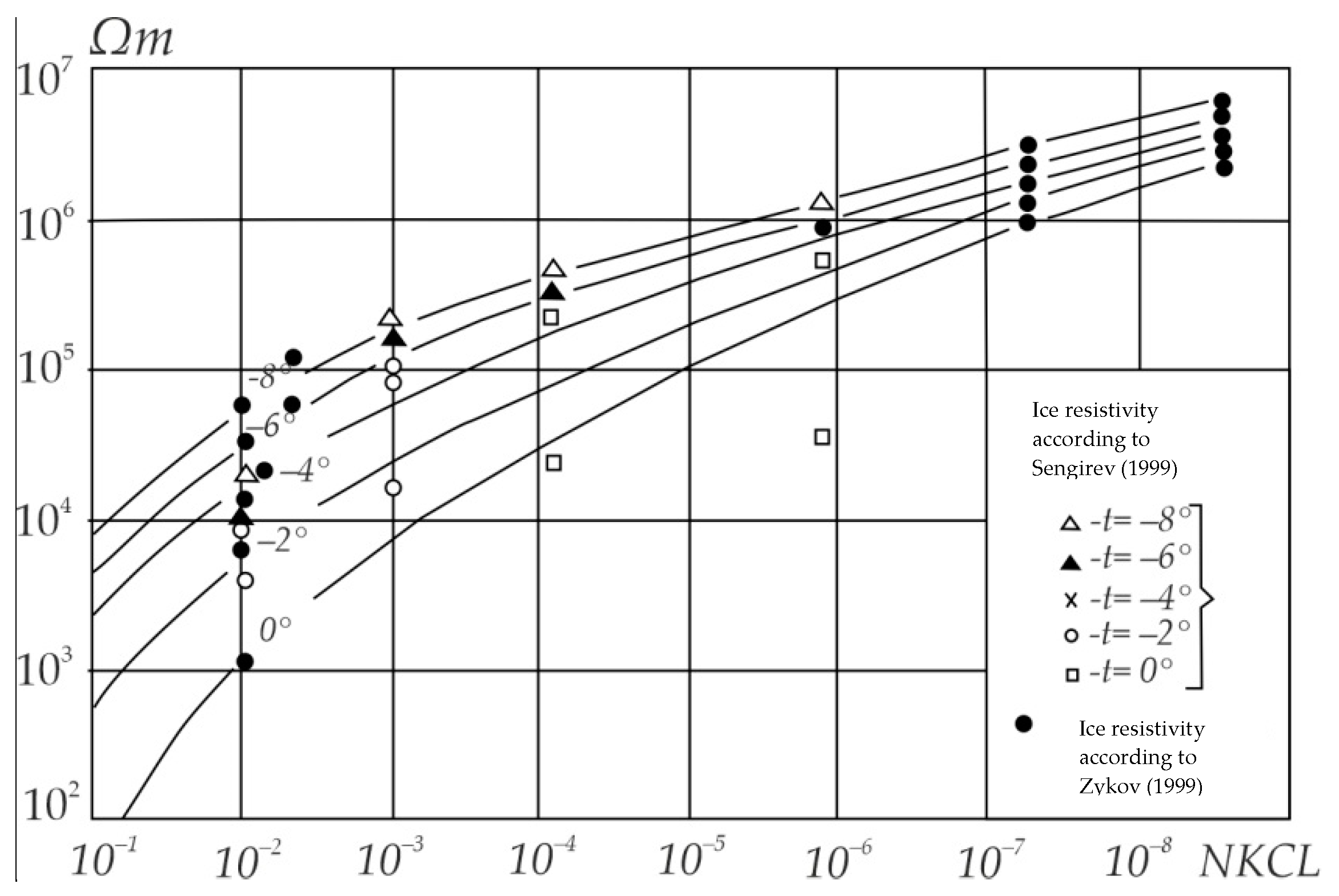
The resistivity of both surface water and rocks depends on groundwater salinity, while the resistivity of ice depends on the salinity of frozen electrolytes and temperature (Figure 3).

The 1D Earth responses from each sounding point were first processed using the forward algorithm developed at the Trofimuk Institute of Petroleum Geology and Geophysics, Siberian Branch of the Russian Academy of Sciences (IPGG, Novosibirsk). The forward solution was obtained with regard to the duration of the current pulse and current turn-off (ramp). The inversion was carried out iteratively, adjusting the resistivity and layer thicknesses until the misfit between the theoretical and field curves reached the minimum. No limitations for changes in layer resistivity were imposed. During the inversion, the induced polarization parameters were taken into account as the Cole–Cole complex frequency-dependent conductivity related to the chargeability, relaxation time, and exponent. The average inversion misfit did not exceed 5%. The results of the sTEM inversion were checked against resistivity logs for the boundaries of geological intervals and sTEM resistivity patterns.

3. Results

The joint action of past and modern hydrogeological factors in the West Siberian Plain has produced three main zones of continuous, discontinuous, and relict permafrost (from north to south) [10,11]. This division was confirmed by geophysical data from central and northern West Siberia, which also allowed mapping of the structure of the area and its geocryological features [13].

sTEM soundings within survey areas were carried out from 2016 to 2021. The TEM curves (voltage decay and apparent resistivity) are shown in Figure 4A for Site 1 and Figure 4B for Site 2, respectively. The parameters of the acquisition were the size of 100 m × 100 m transmitter loops (Tx); compact 5 m × 5 m receiver loops (Rx); offsets of 0 and 100 m; and current strength in transmitter loop up to 30 A.

The sTEM responses from Site 1 (Figure 4I) have a decay duration of 9 ms (Figure 4I(A)), with an apparent resistivity maximum up to 800 Ω·m at 0.02 ms and descending resistivity curve ~20 Ω·m at the late time of decay (Figure 4I(B)).

The Site 2 sTEM curves (Figure 4II) have a longer transient process (Figure 4II(C)) of 40 ms. Minimums of the apparent resistivity curve are evident at 0.03 ms (80 Ω·m), 0.7 ms (20 Ω·m), and 40 ms (10 Ω·m); whereas in the middle part of the curve, resistivity decreases to ~20 Ω·m (Figure 4II(D)).

In both cases, the low-temperature ice-free rocks are displayed on descending branch of the resistivity curve at later times of decay Figure 4I(B),II(D). Inverse problem calculation was applied for sTEM curves within the 1D framework, with the variations in thickness and resistivity of geoelectric layers [8].

The 1D inversion was carried out using the forward algorithm developed at the Trofimuk Institute of Petroleum Geology and Geophysics, Siberian Branch of the Russian Academy of Sciences, Novosibirsk. The duration of the current pulse and current turn-off (ramp) were taken into account. The inversion was applied in a multi-iteration way, changing the resistivity and layer thicknesses. Inversion was accomplished when the misfit between the theoretical and field curves reached the minimum. No limitations for resistivity changes were stated. The induced polarization parameters were calculated applying the Cole–Cole complex frequency-dependent conductivity, which is related to the relaxation time, chargeability, and exponent. The average inversion error was less than 5%. The results of the sTEM inversion were calibrated with resistivity logs from wells at the Sites.

3.1. Results from Site 1

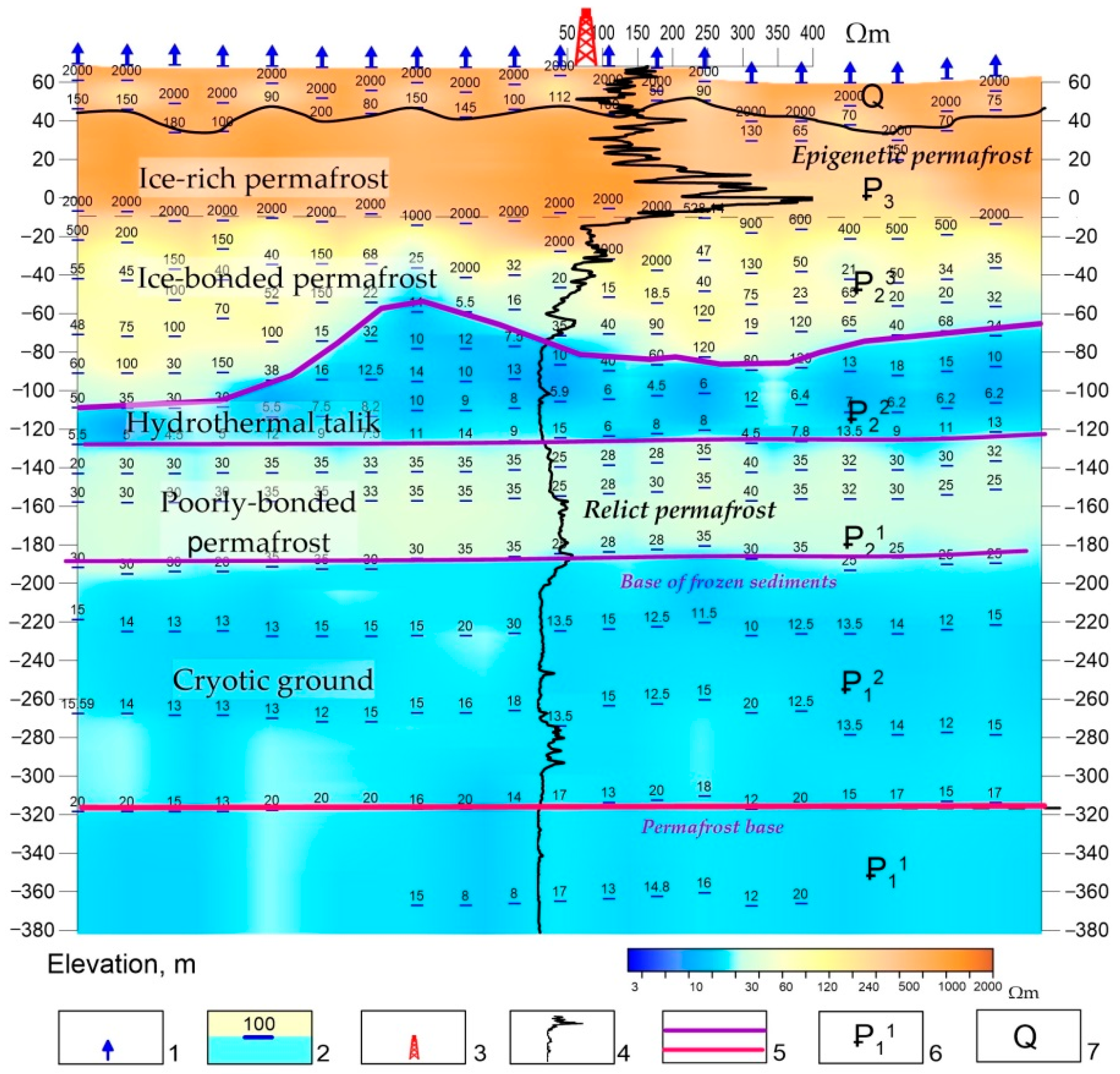
The results of the sTEM resistivity survey at site 1, checked against resistivity and temperature well logs, made the basis for a model of the subsurface to a depth of 500 m. The permafrost comprises two major units common to the southern part of the West Siberian permafrost zone. The upper unit reaches depths of 100 to 180 m (Figure 5) and is further divided into two resistivity layers: ice-rich permafrost, with a temperature around −4 to −5 °C and resistivity of 100 to 2000 Ω·m and −2 °C permafrost with lower ice contents and a lower resistivity of 20 to 200 Ω·m. The two layers together represent thick resistive permafrost, with negative temperatures and moderately high or high ice contents [9].

The modern permafrost lies over a ~20 m-thick layer of unfrozen rocks with a resistivity ≤20 Ω·m. The conductive layer locally reaches a thickness of 50 m, and the permafrost in these areas is most often degraded from above. Drilling in nearby areas confirms the presence of intrapermafrost taliks.

The sTEM images record a layer of 25 to 40 Ω·m resistivity at depths between 170 and 270 m. According to a priori information, the rocks below 250 m are free from visible ice inclusions. The resistivity layer revealed by TEM data may represent relict permafrost, with its base corresponding to the base of frozen sediments.

The modern permafrost has an uneven base (Figure 5), with deeper or shallower local segments. The structure of permafrost and the geometry of its base have several controls. Namely, the permafrost structure depends on local to regional geological (origin, age, lithology, water contents, properties, bedding, and thickness of rocks) and tectonic (neotectonic activity and faults) factors [14].

Sediments could undergo syndepositional freezing in a sea with variable salinity [15]. Local patches of subsea permafrost above a gas pool can merge into large zones and seal gas inside the sediments. Then, while deposition progresses, the permafrost grows upward (syndepositional permafrost), while the frozen sediments below are exposed to the thermal effect of the gas pool [16].

The resistivity cross-sections in the areas of a thicker upper permafrost layer show vertical resistivity features, possibly, associated with gas migration pathways. These areas, located within the zone of metastability, were formerly saturated with hydrocarbons which migrated along conduits and then became sealed up. The presence of hydrocarbons may likewise influence the geometry of the permafrost base. The zones of thick resistive permafrost may store deposits of gas hydrates [9,17,18,19,20,21]. Thus, the permafrost base geometry has formed under the effect of shallow and deep factors.

Reconnaissance surveys in the area and satellite imagery revealed six mounds produced by frost heaving. These pingos were identified during surface surveys of the area, GPS coordinates were taken and then found on a satellite image (4.5 MPixel resolution, source—Bing).

Proceeding from possible relation of heaving to degassing and to deep-seated fluid dynamic processes, the shallow subsurface beneath lakes and heaves was modeled by the inversion of TEM data. Additionally, the results were correlated with seismic data and with known signatures of gas emission [22].

Mound 4 (Figure 6) is especially interesting and hazardous. It is marked by a resistivity anomaly—3–5 Ω·m, which cuts through the permafrost and may record a fluid conduit. Resistivity surveys in the Bovenenkovo oil-gas-condensate field revealed wedge-like thinning of permafrost in fault zones, which may result from heat transfer along zones of weakness and the ensuing temperature disturbance to permafrost [23].

Furthermore, seismic data from the area of mound 4 show a circular anomaly at the depths of Cretaceous strata. Such anomalies detectable in seismic cubes may represent zones of active fluid migration [24]. Therefore, gas migration may occur beneath the mound and may potentially lead to its collapse.

The subsurface immediately beneath mound 5 is free from resistivity or velocity anomalies, but a vertical anomaly (3–5 Ω·m) appears southeast of the mound under a large lake, both in sTEM and seismic images (Figure 6B,D). The anomaly in the seismic section has the appearance of a circular feature. The lake does not correspond to a possible gas emission crater in its present shape and other parameters [22], but it may have changed with time after it formerly filled a carter produced by an explosive gas emission in the past.

The zones of heaving in permafrost may be potential precursors to explosive gas emission events and mark gas emission craters. In this respect, it is essential to image the subsurface beneath such landforms at both shallow and large depths, jointly by several geophysical methods, and to rank them according to size and other parameters.

3.2. Results from Site 2

The subsurface beneath Site 2 is composed of ice-rich permafrost, which appears as a ~250 m-thick layer of relatively high resistivity (20 to 500 Ω·m) in the sTEM data (Figure 7D).

The resistivity pattern of permafrost is heterogeneous, both in depth and laterally, with zones of low resistivity near the surface (3–10 and 10–20 Ω·m) associated with numerous unfrozen zones (taliks) of different types. Many taliks form beneath lakes and rivers (Figure 7) due to the warming effect of water [25]. Resistivity lows (5–10 Ohm·m) are detectable in the maps of surfaces at the 10 m and 50 m depths beneath the Tambei and Nenzotayakha deltas (Figure 7A,B). The inlets of rivers into seas (deltas, estuaries, etc.) produce sub-estuary taliks [13]. A large talik of this kind shows up in the sTEM data as a low-resistivity zone (3–10 Ohm·m) in the Ob Gulf area. The talik results from an intricate interaction of discharged fresh river water with the saline water of the Kara Sea, while the river mouth divides the Ob Gulf into the middle and northern parts.

Other taliks in the area result from the effect of groundwaters that often flow almost vertically down permeable zones of fractures, faults, or karst in carbonate sediments. Such taliks consume water and maintain the recharge of deep groundwaters beneath and within permafrost [25].

The taliks associated with large lakes are marked by resistivity lows, e.g., those in the resistivity maps of the −10 m and −50 m surfaces (Figure 8A,B). The largest and deepest lakes produce isometric anomalies of 5–10 Ω·m that reach the permafrost base (Figure 8D).

The territory of northern West Siberia abounds in thermokarst (thaw) lakes, which often become sources of methane emission into the atmosphere. Gas emitted from permafrost in the Yamal Peninsula is of biogenic or thermogenic origin [26].

Ongoing tectonic movements [23,26], especially active faults, including degassing features, are often expressed geomorphically. Many large and small rivers follow faults (e.g., in the Novy Port, Taz, and other oil and gas fields), while lakes can form above fault intersections (e.g., Lake Neito). The sTEM geoelectric patterns obtained for the area show resistivity lows beneath most of the large lakes (Figure 8). The same zones correspond to large and small faults inferred from resistivity contrasts. Such anomalies, detectable in resistivity maps and cross-sections, are zones of degassing faults and related lakes with degassing signatures.

Thus, the structure of permafrost imaged by sTEM surveys at two sites of northern West Siberia (the northeastern Yamal Peninsula and the southern Gydan Peninsula) is quite heterogeneous, with numerous near-surface, intrapermafrost, and subpermafrost unfrozen zones. The resistivity and seismic anomalies detectable beneath lakes and frost heaves may trace gas migration pathways. This inference supports the idea that cryogenic landforms can be considered indicators of the degassing associated with deep-seated fluid dynamic processes in the Arctic.

4. Conclusions

TEM surveys were carried out to investigate permafrost in two completely different regions of Western Siberia.

For the first time, an electromagnetic method was applied to build a model of two-layered permafrost (high resistivity) separated by a talik (low resistivity) within site No. 1 (the central part of Western Siberia). The first permafrost layer (modern permafrost) was mapped at depths of 100–180 m. The thickness of the talik is about 20 m. The second permafrost layer (relict permafrost) was observed at depths of 170–270 m.

Areas of the supposed gas hydrates accumulation under the modern permafrost layer (high-resistivity pockets) have been identified. Based on on-site surface studies, seismic and TEM surveys, and satellite images, pingos were examined as resistivity and seismic anomalies associated with gas migration channels. Such studies are unique for their kind.

At site No. 2 (northern Yamal), TEM was applied to investigate the complex structure of the Yamal Peninsula permafrost to identify a thick layer of permafrost in the section. The permafrost sequence has a heterogeneous structure. Against the background of high-resistivity permafrost (20–500 Ω·m), there is a large number of “hydrogenous taliks”, as well as through thawed zones characterized by low resistivity (3–10 Ω·m). The area of hydrogen taliks covers from 5–50 m² (under rivers and lakes) to 80 m² (under-estuary talik). It is crucial to drill verification wells in areas, with core sampling and temperature logging, as well as wells in areas where gas hydrates are expected to accumulate.

The reported results of shallow, transient electromagnetic surveys demonstrate the applicability of the method to the studies of permafrost. The TEM data, which can be correlated with seismic and remote sensing data, resolve tectonic faults as channels of migrating fluids and frost heaving features as potential indicators of gas hydrates fields.

Monitoring oil and gas fields using different geophysical methods, including electromagnetic soundings, is important to image the permafrost structure and thus predict and mitigate risks associated with explosive gas emissions, which may damage people and infrastructure.

The collected sTEM data can be used as references for further monitoring of permafrost in the Arctic petroleum provinces.

References

- Lévesque, Y.; Walter, J.; Chesnaux, R. Transient Electromagnetic (TEM) Surveys as a First Approach for Characterizing a Regional Aquifer: The Case of the Saint-Narcisse Moraine, Quebec, Canada. Geosciences 2021, 11, 415. [Google Scholar] [CrossRef]
- Spichak, V.V. Electromagnetic Sounding of the Earth’s Interior, 2nd ed.; Elsevier: Amsterdam, The Netherlands, 2015. [Google Scholar] [CrossRef]
- Zykov, Y.D. Geophysical Methods of Permafrost Studies; Moscow University Press: Moscow, Russia, 1999; 243p. [Google Scholar]
- Yakupov, V.S. Geophysics of the Cryolithozone; Izdat-vo Yakutskogo un-ta: Yakutsk, Russia, 2008; 342p. [Google Scholar]
- Ogil’vi, A.A. Fundamentals of Engineering Geophysics; Nedra: Moscow, Russia, 1990; 501p. [Google Scholar]
- Yakovlev, D.V.; Yakovlev, A.G.; Valyasina, O.A. Permafrost study in the northern margin of the Siberian platform based on regional geoelectric survey data. Kriosf. Zemli 2018, XXII, 77–95. [Google Scholar] [CrossRef]
- Olenchenko, V.V.; Shein, A.N. Geocryology of floodplain and above-floodplain deposits of the Yuribei River (Yamal Peninsula): Evidence from resistivity surveys. In Proceedings of the Interexpo Geo-Sibir, Novosibirsk, Russia, 17–19 April 2012; Volume 1, pp. 33–37. [Google Scholar]
- Buddo, I.; Sharlov, M.; Shelokhov, I.; Misyurkeeva, N.; Seminsky, I.; Selyaev, V.; Agafonov, Y. Applicability of Transient Electromagnetic Surveys to Permafrost Imaging in Arctic West Siberia. Energies 2022, 15, 1816. [Google Scholar] [CrossRef]
- Misurkeeva, N.V.; Buddo, I.V.; Smirnov, A.S.; Shelokhov, I.A. Shallow Transient Electromagnetic Method Application to Study the Yamal Peninsula Permafrost Zone. In Proceedings of the Geomodel 2020, Gelendzhik, Russia, 7–11 September 2020; pp. 1–6. [Google Scholar]
- Baulin, V.V.; Belopulhova, E.B.; Dubikov, G.I.; Shmelev, L.M. Geocryological Conditions in the West Siberian Plain; Nauka: Moscow, Russia, 1967; 214p. [Google Scholar]
- Ershov, E.D. (Ed.) Geocryology of the USSR. West Siberia; Nedra: Moscow, Russia, 1989; 454p. [Google Scholar]
- Baulin, Y.I.; Bogolubov, A.N.; Zykov, Y.D. Recommended Practice for the Use of Geophysical Methods for the Determination of the Geological Engineering Characteristics of Frozen Fine-Grained Soils; Stroiizdat: Moscow, Russia, 1984; 32p. [Google Scholar]
- Misyurkeeva, N.V.; Buddo, I.V.; Shelokhov, I.A.; Agafonov, Y.A. Heaving model, from electromagnetic data. In Proceedings of the KHKHVII Russian Early-Carrier Conference with International Contributions, Irkutsk, Russia, 22–28 May 2017; Institute of the Earth’s Crust: Irkutsk, Russia, 2017; pp. 151–152. [Google Scholar]
- Romanovsky, N.N. Fundamentals of Cryogenesis in the Lithosphere; Moscow University Press: Moscow, Russia, 1993; 336p. [Google Scholar]
- Badu, Y.B.; Podborny, E.E. Permafrost thickness. In The Cryosphere in the Area of Oil-Gas-Condensate Fields of the Yamal Peninsula. Book 2. Bovanenkovo Oil-Gas-Condensate Field; Gazprom Exspo: Moscow, Russia, 2013; pp. 391–414. [Google Scholar]
- Badu, Y.B. Permafrost in Gas Reservoirs of the Yamal Peninsula. Effect of Gas Fields on the Origin and Evolution of Permafrost; Scientific World: Moscow, Russia, 2018. [Google Scholar]
- Chuvilin, E.M. Stroenie i svojstva porod kriolitozony yuzhnoj chasti Bovanenkovskogo gazokondensatnogo mestorozhdeniya/E.M. CHuvilin, E.V. Perlova, YU.B. Baranov i dr. GEOS 2007, 137s, 74–113. [Google Scholar]
- Chuvilin, E.M.; Davletshina, D.A.; Lupachik, M.V. Gidratoobrazovanie v merzlyh i ottaivayushchih metanonasyshchennyh porodah. Kriosf. Zemli 2019, XXIII, 50–61. [Google Scholar] [CrossRef]
- Yakushev, V.S.; Perlova, E.V.; Mahonina, N.A.; CHuvilin, E.M.; Kozlova, E.V. Gazovye gidraty v otlozheniyah materikov i ostrovov. Ros. Him. Zh. 2003, XLVII, 80–90. [Google Scholar]
- Yakushev, V.S. Prirodnyj Gaz i Gazovye Gidraty v Kriolitozone; M. VNIIGAZ: Moscow, Russia, 2009; 192 s. [Google Scholar]
- Afanasenkov, A.P.; Volkov, R.P.; Yakovlev, D.V. Anomalii povyshennogo elektricheskogo soprotivleniya pod sloem mnogoletnemerzlyh porod—novyj poiskovyj priznak zalezhej uglevodorodov. Geol. Nefti I Gaza 2015, 6, 40–51. [Google Scholar]
- Bogoyavlensky, V.I.; Sizov, O.S.; Bogoiavlensky, I.V.; Nikonov, R.A.; Kargina, T.N. Degassing in the Arctic: Integrated studies of frost heaves, thermokarst lakes, and gas-emission craters in the Yamal Peninsula. Nauchnye Issled. V Arktike 2019, 4, 52–68. [Google Scholar]
- Skorobogatov, V.A.; Stroganov, L.V.; Kopeev, V.D. Tectonic history and the present structure of the absement and sediments in the Yamal area. In Geology and Petroleum Potential of the Yamal Peninsula; Nedra: Moscow, Russia, 2003; 352p. [Google Scholar]
- Nezhdanov, A.A.; Novopashin, V.F.; Ogibenin, V.V. Mud volcanism in northern West Siberia. In Geology and Exploration. Collection of Papers. OOO TyumenNIIgiprogaz; Flat: Tyumen, Russia, 2011; pp. 73–79. [Google Scholar]
- Romanovsky, N.N. Taliks in Permafrost and Their Classification. Bull; Moscow University: Moscow, Russia, 1972; pp. 23–34. [Google Scholar]
- Bondarev, V.L.; Mirovskiy, M.Y.; Zvereva, V.B.; Oblekov, G.I.; Shaidullin, R.M.; Gudzenko, V.T. Gas-geochemical characteristics of the Nadsenomanian deposits of the Yamal Peninsula (on the example of the Bovanenkovsky oil and gas condensate field). Geol. Geophys. Dev. Oil Gas Fields 2008, 5, 22–34. [Google Scholar]