Experimental Performance Analysis of Adsorption Modules with Sintered Aluminium Fiber Heat Exchangers and SAPO-34-Water Working Pair for Gas-Driven Heat Pumps: Influence of Evaporator Size, Temperatures, and Half Cycle Times

Abstract

A major challenge for gas-driven adsorption heat pumps is the production of compact, efficient, and cost-effective adsorption modules. We present the experimental data of a design based on sintered aluminum fiber heat exchangers, a technology currently under development. The adsorption module presented here is the result of the downsizing of a larger module. The downsized module has an adsorption heat exchanger that is 60% of the size of the larger-scale component, and an evaporator-condenser that is only 30% of the size of the larger-scale component. It is designed to fit the heating requirements of a wall-hung heat pump for a single-family home. For the first time, a comprehensive experimental study of the influence of half-cycle time, evaporator and adsorption temperature, and driving temperature on the efficiency and power of the module is presented. At temperature conditions relevant for the application of a gas-driven adsorption heat pump, i.e., evaporator temperature < 10 °C and adsorption temperature > 30 °C, we found that the downsizing has its price in terms of a higher thermal capacity of the components in relation to the adsorbent mass (9.6 kJ/(kg∙K) for ‘Size S’) vs. 5.6 kJ/(kg∙K) for ‘Size L’). We carried out an evaluation of heat and mass transfer resistances to compare the ‘Size L’ module directly with the ‘Size S’ module. Both modules have nearly the same volume-scaled heat and mass transfer resistances of 0.012 dm³ K/W (adsorption heat exchanger during adsorption) and 0.005 dm³ K/W (evaporator–condenser during evaporation), and consequently a very similar volumetric power density. This evaluation proves the applicability and the consistency of the concept of heat and mass transfer resistances, and the scalability of this adsorption module technology.

1. Introduction

According to Kemna et al. [1] wall-hung condensing gas boilers are the most widely used technology for domestic heating and hot water supply in Germany and Europe (>4 million units sold per year in Europe). A reduction in CO₂ emissions can only be achieved with further improvement the efficiency of heating technology, or with decreasing demand. The efficiency of burning gas with a condensing gas boiler is at its maximum—it cannot be improved further. With gas-driven adsorption heat pumps, the efficiency can be improved—the resulting needs for this market segment are compact, efficient, and cost-effective adsorption modules. The development of gas-driven adsorption heat pumps (GAHP) made remarkable progress in the years 2009 to 2013, when companies such as Vaillant and Viessmann presented their GAHP products based on the zeo-type material SAPO-34/water working pair [2,3,4]. Another related development with a similar technology readiness level is the GAHP working with an activated carbon/ammonia working pair [5,6]. Besides these developments on the appliance level or adsorption module level, much effort has also been made on the component-development level. Mikhaeil et al. [7] present an adsorption heat exchanger based on the plate heat exchanger geometry, with loose grains of AQSOA-Z02 (similar to SAPO-34). Saleh et al. [8] compare a wire-fin heat exchanger with a finned-tube heat exchanger and a microchannel heat exchanger. All measured heat exchangers are filled with loose grains of the metal–organic framework material aluminium fumarate. Seol et al. [9] present measurements of an adsorption heat exchanger based on flat tubes and lamellas (or fins) that are coated with a novel binder based adsorbent. The geometry is similar to the adsorption heat exchanger used by Bendix et al. [10] in combination with a binder-based SAPO-34 coating. This kind of heat exchanger was used by Kowsari et al. [11] in combination with loose grains of SWS-1L. More recently, Calabrese et al. [12] presented a heat exchanger on a polymer basis (SPEEK) coated with SAPO-34. Some small scale measurements with different polymer supports were presented earlier by Hinze et al. [13]. These works aimed to reduce the thermal capacity of the adsorption heat exchanger, which is crucial for increasing efficiency [14]. This non-exhaustive list focuses on the most recent publications on the component development level. More information can be found in the recent review by Caprì et al. [15].

The design of the adsorption heat exchanger and the evaporator–condenser presented here is based on flat tubes with fibrous structures that are directly crystallized with SAPO-34 [16,17,18]. The crystallization on the aluminium surface is carried out with the partial support transformation (PST) technique presented by Bauer et al. [19]. Measurements on such an adsorption module (named ‘Size L’ in the following) were first presented by Wittstadt et al. [17]. This module had an adsorbent mass of 3.3 kg, a volume of 34.3 dm³, and an average thermal power output of 12 kW (adsorption half cycle at 15/35/90 °C) [17], which is far too much for a wall-hung gas adsorption heat pump with a nominal heating capacity of 10 kW. For such a device, the average thermal power output of the adsorption module should be around 6–8 kW, since most of the heating will be provided at part-load. Based on the results of Wittstadt et al. [17], we downsized the adsorption heat exchanger to 60% of the size of the ‘Size L’ component to achieve a thermal power output in this range. The further downsizing of the evaporator–condenser to 30% is based on the findings of Wittstadt et al. [17] regarding the overall heat and mass transfer resistances (given as UA-values, which are the reciprocal resistances). The results indicated that the evaporator–condenser has a low overall heat and mass transfer resistance compared to the adsorption heat exchanger. Thus, downsizing to 30% would lead to balanced overall heat and mass transfer resistances of the components without decreasing the average thermal output of the ‘Size S’ module significantly. The experimental results presented by Wittstadt et al. [17] lack temperature conditions relevant for the application of a gas-driven adsorption heat pump, i.e., evaporator temperature <10 °C and adsorption temperature > 30 °C. To close this gap, we present a comprehensive study of the influence of half cycle time, evaporator temperature, adsorption temperature and also driving temperature on the efficiency and power of the ‘Size S’ module here.

It is worth noting that this kind of adsorption module differs from the module used by Viessmann in their GAHP (see publication of Dawoud [3] for details), not only in component design but also in the arrangement of the components. The module presented here has a combined evaporator–condenser component, while the Viessmann adsorption module has a separate evaporator and a separate condenser [14]. The advantages of the combined component are that only a single component is needed, and that it is not necessary to separate it from the adsorption heat exchanger. However, the major disadvantage is the negative impact on the efficiency, since the heating up of the thermal capacity of the evaporator–condenser consumes useful energy during the switching phase from evaporation to condensation [18]. For this reason, it is important to lower the thermal capacity of the combined component to increase the efficiency [18]. In the design of the adsorption module presented here (named ‘Size S’ in the following), we tried to tackle two points:

• Downsize the module to fit into a wall-hung gas adsorption heat pump. The target volume for such an application is between 10 and 15 dm³.
• Downsize the thermal capacity of the evaporator–condenser without having a negative impact on the power density.

The question arises on which basis two modules of different sizes with similar components should be compared. The most obvious basis is the comparison of efficiency and power density with the same temperature conditions. A targeted optimization requires an understanding of the limiting processes. Thus, it is desirable to find out which component limits the process or better: which heat and mass transfer process in which component limits the process [14]. The basis for such an analysis was presented by Wittstadt et al. for adsorption modules [20], Velte et al. [21] for small scale samples, and later Schnabel et al. [14] by evaluating driving temperature equivalents. This method was developed further and used by Wittstadt et al. [17] to calculate overall UA-values for the adsorption heat exchanger and the evaporator–condenser. Wittstadt [22] uses this method for the identification of heat and mass transfer resistances of a directly crystallized finned (round) tube heat exchanger. Ammann et al. [23,24] presented a similar approach for the quantification of heat and mass transfer resistances on the basis of measurements on small scale samples. Seol et al. [9] recently calculated driving temperature equivalents for the evaluation of adsorption heat exchanger measurements, and tried to differentiate between heat and mass transfer by acquiring the adsorbent temperature of the adsorption heat exchanger. However, the applicability and the consistency of this approach when it comes to adsorption modules with different sizes has not been shown yet in literature. In this paper we provide a concise description of the evaluation of heat and mass transfer resistances out of the measurement data that we gained on the adsorption module level. We show how to use this data for a rigorous performance evaluation and identification of the component limiting the process. Furthermore, we use volume-scaled heat and mass transfer resistances to compare the components and adsorption modules of different sizes.

Besides the heat and mass transfer resistances of the components, the capacity flow of the heat transfer fluid (HTF) also plays a role in the study of the dynamics of an adsorption heat exchanger—basic heat-exchanger theory and related dimensionless numbers, e.g., the number of transfer units (NTU) can help to analyse and compare the performance of heat exchangers [25,26]. Although Miyazaki et al. [27] evaluated different dimensionless numbers to study their influence on the cycle time of an adsorption chiller, they focused only on the heat transfer resistances of the components that can be obtained by using correlations and estimates for heat transfer coefficients. This evaluation of a “thermal NTU” can be helpful, but it is only a part of the picture, since mass transfer plays a role in the adsorption heat exchanger. Our approach of evaluating heat and mass transfer resistances overcomes this limitation with the calculation of an overall NTU of the adsorption heat exchanger, including the mass transfer processes.

2. Materials and Methods

2.1. Adsorption Module

The adsorption module is based on sintered fiber heat exchangers as presented by Wittstadt et al. [17]. The main difference between the module presented by Wittstadt et al. [17] (‘Size L’) and the module studied here (‘Size S’) is the size of the components. The main geometric data is listed in

Table 1. Main data of the components and the modules.

Quantity	Size L	Size S
Adsorption heat exchanger
Adsorbent mass in kg	3.3 ± 0.3	1.5 ± 0.2
Heat exchanger dimensions in mm with headers w/o headers	700 × 313 × 45 600 × 313 × 45	450 × 185 × 80 400 × 185 × 80
Volume in dm3 with headers	9.9 ± 0.1	5.7 ± 0.1
Evaporator–condenser
Heat exchanger primary area in m2	43 ± 2	14 ± 1
Heat exchanger dimensions in mm with headers w/o headers	700 × 313 × 45 600 × 313 × 45	450 × 158 × 45 400 × 158 × 45
Volume in dm3 with headers	9.9 ± 0.1	3.2 ± 0.1
Module
Dimensions in mm (w/o insulation)	730 × 320 × 147	474 × 169 × 188
Volume in dm3 (w/o insulation)	34 ± 0.2	15 ± 0.2

, and a picture of the ‘Size S’ module is shown in Figure 1. Please note that the data in Table 1 was earlier presented by the author in the conference proceedings of the International Sorption Heat Pump Conference 2021 [28], and is listed here again for convenience. The new module was designed with a smaller condenser/evaporator component in order to decrease the thermal mass of this component. Lowering the thermal mass of the combined condenser/evaporator increases the efficiency, due to the reduction in energy consumed during the switching phase from evaporation to condensation, and vice versa.

We calculated the thermal capacities of the components according to the method presented by Gluesenkamp et al. [29]. The resulting thermal capacities are shown in Figure 1 (left). The new condenser/evaporator of module ‘Size S’ is much smaller and has a much lower total thermal capacity than the one presented by Wittstadt et al. [17]. Although it was designed to be even smaller, it is remarkable that the total thermal capacity of this component is only 40% of the component presented by Wittstadt et al. [17]. However, the cost of downsizing is a decrease in the ratio of primary area and thermal capacity, which is approximately 2.5 m² K/kJ for the ‘Size L’ module and approximately 2 m² K/kJ for the ‘Size S’ module. we see a similar dependence in the case of the adsorption heat exchanger. The ‘Size L’ component has an adsorbent mass specific thermal capacity of 5.6 kJ/(kg∙K) and the ‘Size S’ component has a specific thermal mass of 9.6 kJ/(kg∙K) which is a disadvantage in terms of efficiency for the ‘Size S’ module.

For further evaluation we listed some additional geometric data of the heat exchangers of the ‘Size S’ module in

Table 2. Additional geometric data of ‘Size S’ module.

Quantity		Value
Adsorption heat exchanger
Inner area of flat tube in m2	$A_{i,tb}$	1.17
Contact area between fibres and tubes in m2	$A_{tb,fib}$	0.63
Thickness of fibrous structure between two flat tubes in mm	$d_{fib}$	10
Number of flat tubes	$n_{tbs}$	12
Height of the component (=width of flat tube) in mm	$h_{ADHX}$	80
Evaporator-condenser
Inner area of flat tube in m2	$A_{i,tb}$	0.58
Contact area between fibres and tubes in m2	$A_{tb,fib}$	0.39
Thickness of fibrous structure between two flat tubes in mm	$d_{fib}$	10
Number of flat tubes	$n_{tbs}$	12
Height of the component (=width of flat tube) in mm	$h_{EC}$	45

. The adsorption heat exchanger has a larger width of the flat tubes and fibrous structures than the evaporator-condenser. Consequently, the inner area of the flat tubes and the contact area between fibrous structure and flat tubes of the evaporator-condenser are smaller. The number of the flat tubes and also the thickness of the fibrous structures are the same for both components.

The evaporator-condenser metal remained untreated due to manufacturing limitations. As soon as the untreated aluminium surface is exposed to water a corrosion process with the formation of hydrogen starts. This was the case during the measurements with water as working fluid. The hydrogen formation leads to an increase of hydrogen partial pressure within the module. This pressure increase was around 0.1…0.3 mbar within a complete cycle (350…900 s). To maintain a pure water vapour atmosphere, the valve to the vacuum pump was opened at the end of each desorption half cycle for 2–5 s. Despite these corrosion problems the measurements showed a quite good reproducibility as detailed in Section 3.4.

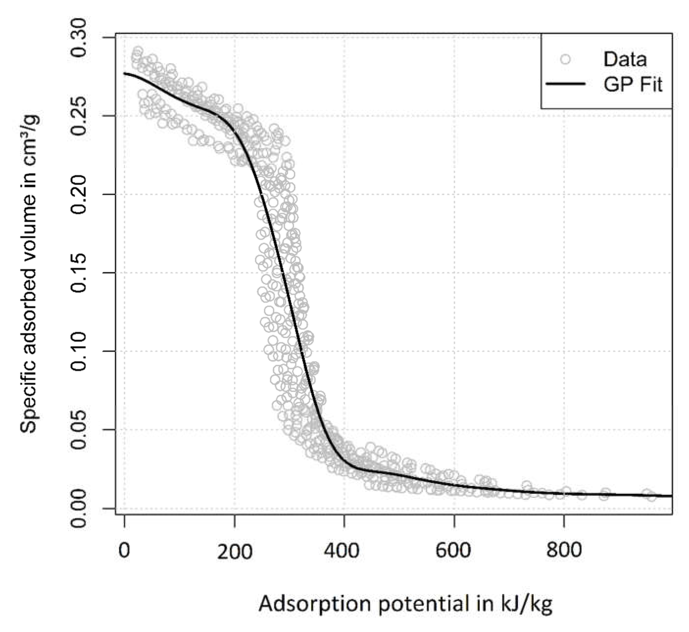
2.2. Adsorption Equilibrium Data

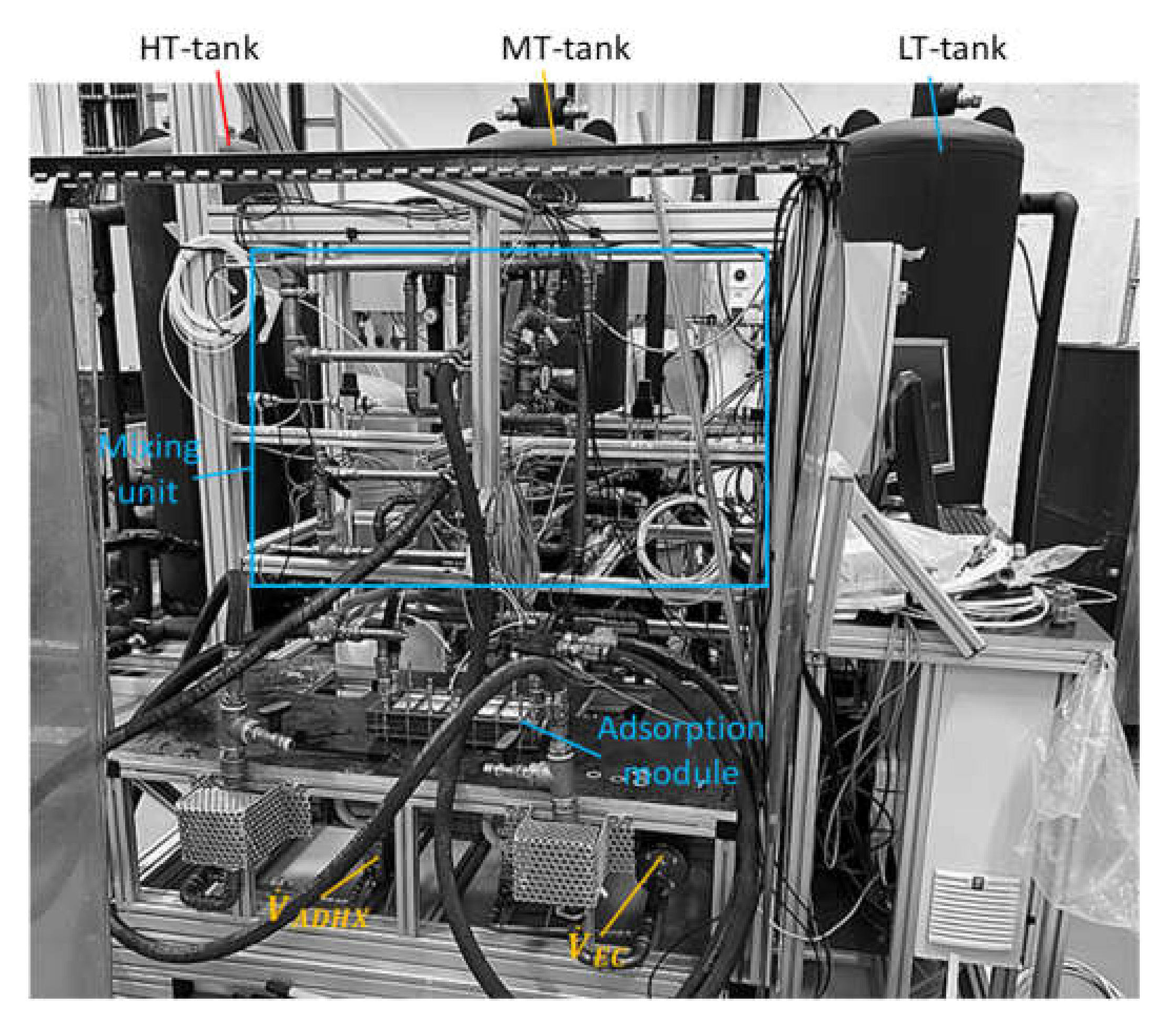
For the measurement of the adsorption equilibrium a flat plate sample with directly crystallized SAPO-34 was prepared and measured with a volumetric device at different temperature levels (ranging from 20.1 °C and 121.7 °C) by the manufacturer (Fahrenheit GmbH, Halle (Saale), Germany). Each obtained isotherm consists of at least 15 different measured points. The measured data are shown in Dubinin’s representation in Figure 2—the measured loading $X$ is transformed to the specific adsorbed volume $W=X/{\rho }_{ad}$ and the measured pressure $p$ and temperature $T$ are expressed as the adsorption potential $A=RT\cdot \ln \left(p_{sat}/p\right)$. We followed the approach of Desai et al. [31] to obtain a characteristic curve W(A) with Gaussian Process Regression which is shown as “GP Fit” in Figure 2. Although the required temperature invariance criterion is not fulfilled for the directly crystallized SAPO-34, the RMSD between measured loading $X_{eqi}$ and calculated loading is 0.028 kg/kg. For evaluating heat and mass transfer resistances this an acceptable deviation.

2.3. Test Rig

The test rig for adsorption modules at Fraunhofer ISE as shown in Figure 3 consists of three storage tanks at different temperature levels, two pumps for adsorption heat exchanger and condenser/evaporator hydraulic circuits, temperature sensors, flow sensors, and several valves to control the inlet temperature of the components as shown schematically in Figure 3 and figuratively in Figure 4. The main signals that we use for the evaluation of the adsorption module measurements are listed below:

• The inlet and outlet temperatures of the adsorption heat exchanger and the evaporator-condenser. These temperatures are measured with pairwise calibrated Pt-100 sensors, TMG, with a measurement uncertainty of ±0.01 K.
• The volume flow rates of the evaporator-condenser and the adsorption heat exchanger are measured with volume flow sensors (Proline Promag 50P, Endress + Hauser, Germany, DN25), the uncertainty of the measured velocity is ±0.5% of the measured value ±1 mm/s.
• The pressure of the module with a capacitive pressure sensor (MKS Baratron 627B, Andover, MA, USA).
• The temperature of the housing at three different locations is measured with Pt-100 thin film sensors, ±0.3 K.

2.4. Evaluation of Efficiency and Power Density

The energy balances of the HTF cycles are shown in Equations (1) and (2), respectively. This yields the heat transferred from the HTF into the module during desorption and evaporation and vice versa during adsorption and condensation. The data for the enthalpy $h_L$, the density ${\rho }_L$, and the specific heat capacity are calculated according to the IAPWS 97 formulation [32] with a script implemented by Holmgren [33].

$${\dot{Q}}_{EC}={\dot{M}}_{HTF,EC}\cdot \left(h_L\left(T_{EC,out}\right)-h_L\left(T_{EC,in}\right)\right)\approx {\rho }_{L,HTF}\left(T_{EC,out}\right)\cdot {\dot{V}}_{HTF,EC}\cdot {\overline{c}}_{p,L}\cdot \left(T_{EC,out}-T_{EC,in}\right).$$

(1)

$$\begin{gathered} {\dot{Q}}_{adHX}={\dot{M}}_{HTF,adHX}\cdot \left(h_L\left(T_{adHX,out}\right)-h_L\left(T_{adHX,in}\right)\right) \\ \approx {\rho }_{L,HTF}\left(T_{adHX,out}\right)\cdot {\dot{V}}_{HTF,adHX}\cdot {\overline{c}}_{p,L}\cdot \left(T_{adHX,out}-T_{adHX,in}\right). \end{gathered}$$

(2)

The integration of Equation (2) over the adsorption or desorption half cycle yields the amount of energy for adsorption $Q_{ads}$ and desorption $Q_{des}$. Accordingly, the integration of Equation (1) yields the amount of energy for evaporation $Q_{evap}$ and condensation $Q_{cond}$. In this formulation $Q_{ads}$ and $Q_{cond}$ have a negative sign whereas $Q_{des}$ and $Q_{evap}$ have a positive sign.

The efficiency for the heating application is calculated according to Equation (3) with the heat released during adsorption and condensation and the heat transferred to the module during desorption.

$$CO{P}_{heat}=\frac{-Q_{ads}-Q_{cond}}{Q_{des}}.$$

(3)

Another important quantity is the volume specific heating power VSHP that is calculated according to Equation (4). This quantity relates the heating power and the volume of the module.

$$VSH{P}_{heat}=\frac{-Q_{ads}-Q_{cond}}{\left(t_{hlfCyc,ads}+t_{hlfCyc,des}\right)\cdot V_{mod}}.$$

(4)

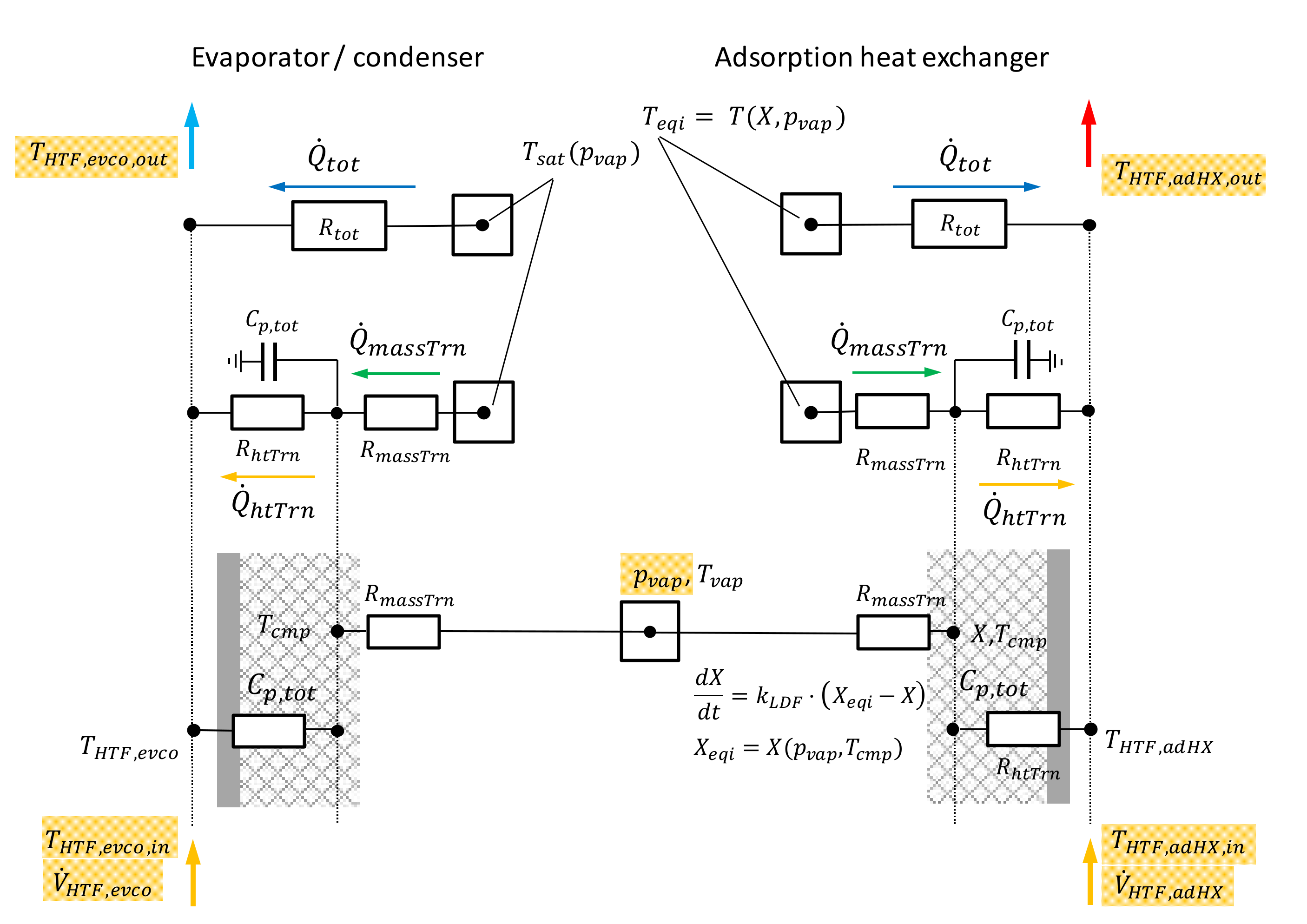
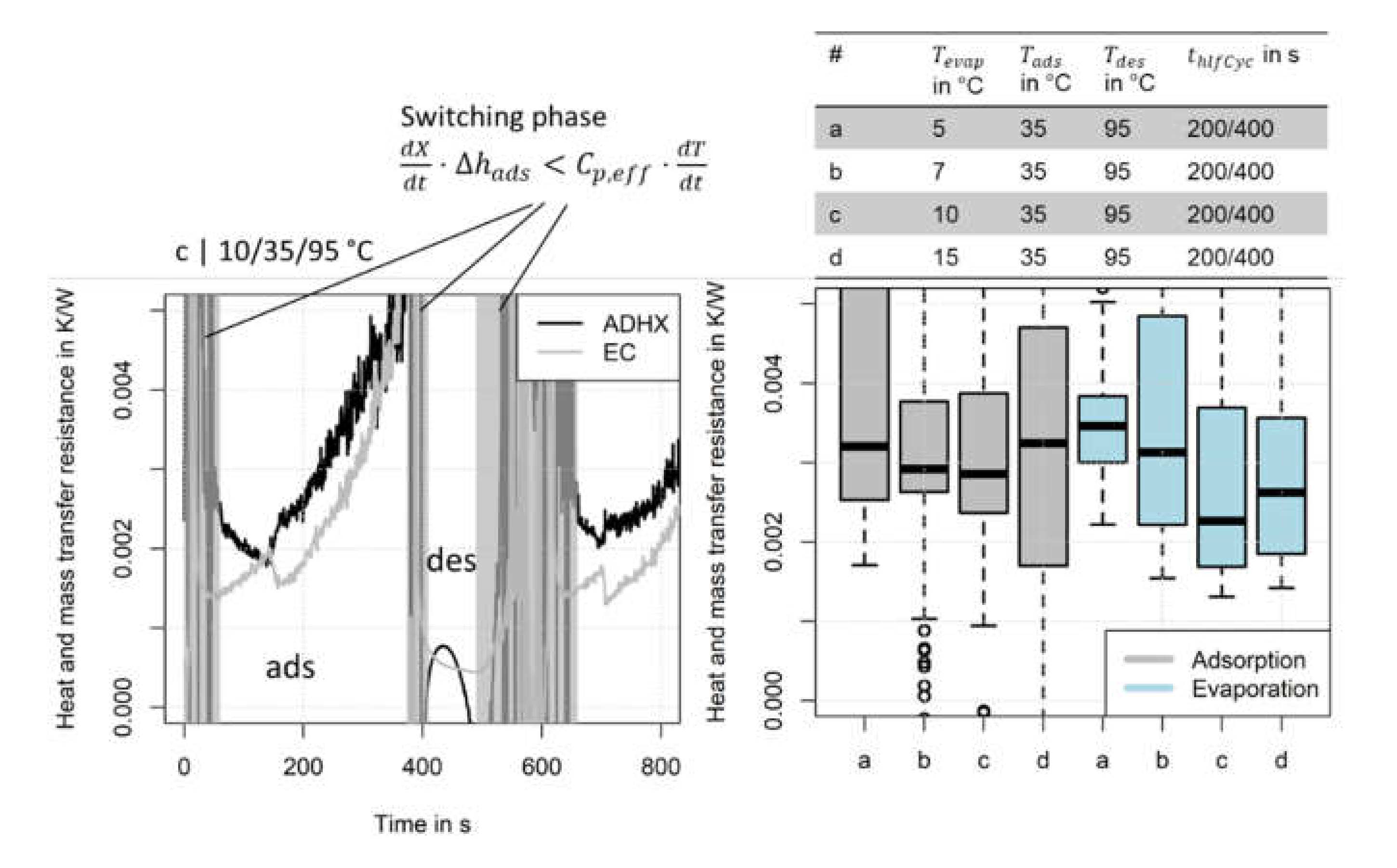
2.5. Evaluation of Heat and Mass Transfer Resistances

The measurement of adsorption modules and the evaluation of efficiency and power density can help to judge whether a specific design A is more efficient or has a higher power density than another design B. For a targeted optimization of the component size as carried out by Lanzerath et al. [34] or component design optimization as carried out by Velte [18] with a numerical model it is important to know which component and better, which heat or mass transfer mechanism within the component is limiting the process.

In Figure 5 the heat and mass transfer resistance model is shown. The measured state variables are marked yellow.

From basic heat exchanger theory we know that the heat flux is related to an overall heat conductance UA_tot and the logarithmic mean temperature difference according to Equation (5) [25].

$${\dot{Q}}_{HTF,adHX/EC}={\left(UA\right)}_{tot}\cdot \mathsf{\Delta }{T}_{mean} .$$

(5)

The logarithmic mean temperature difference is calculated with the in- and outlet temperatures T′ and T″ of the heat exchanger according to Equation (6). In case of condensation or evaporation it is $T_1^{\prime }=T_1^{″}=T_{sat}\left(p\right)$ and Equation (6) can be simplified in the shown way. This holds true approximately also for adsorption and desorption where $T_1^{\prime }=T_1^{″}=T_{eqi}\left(X,p\right)$

$$\mathsf{\Delta }{T}_{mean}=\frac{T_1^{″}-T_2^{\prime }-\left(T_1^{\prime }-T_2^{″}\right)}{\ln \frac{T_1^{″}-T_2^{\prime }}{T_1^{\prime }-T_2^{″}}}=\frac{T_2^{″}-T_2^{\prime }}{\ln \frac{T_{sat}\left(p \right)-T_2^{\prime }}{T_{sat}\left(p\right)-T_2^{″}}}.$$

(6)

Although Equations (5) and (6) are valid for stationary processes, they can be used as a good approximation for UA_tot during the “isobaric” phases of the ad- or desorption half cycle if $C_{p,eff}\cdot dT/dt<\mathsf{\Delta }{h}_{ads}\cdot dX/dt$.

According to Equation (5) we can calculate an overall heat and mass transfer resistance of the component as the reciprocal value of the overall heat conductance as done by Wittstadt et al. [17].

$$R_{tot}=\frac{\mathsf{\Delta }{T}_{mean}}{{\dot{Q}}_{HTF,adHX/evco}} .$$

(7)

The saturation temperature T_sat can be calculated directly out of the measured pressure. For the calculation of the equilibrium temperature T_eqi(X,p) it is necessary to calculate the actual mean loading $X_{xpr}$ of the adsorbent in the adsorption heat exchanger. The function $T_{eqi}\left(X_{xpr},p_{mod}\right)$ is the inverse function of the adsorption equilibrium description $X\left(T,p\right)$. We use the characteristic curve $W\left(A\right)$ to calculate the adsorption equilibrium as described in Section 2.2.

To calculate the experimental loading $X_{xpr}$ we make use of the energy balances of the components. The thermodynamic state of the heat exchanger is described with a single temperature node $T_{ADHX/EC}$. The energy balance of the heat exchanger is given in Equation (8). The first term on the left-hand side accounts for the inner energy of the heat exchanger metal, adsorbent, and working fluid. The second term on the left-hand side accounts for the thermal mass of the HTF.

$$\frac{\partial U_{str,ADHX/EC}}{\partial t}+\frac{\partial H_{HTF,ADHX/EC}}{\partial t}={\dot{Q}}_{HTF,ADHX/EC}+{\dot{Q}}_{src/snk}+{\dot{Q}}_{loss,ext}+{\dot{Q}}_{loss,int}.$$

(8)

The heat flux from the HTF ${\dot{Q}}_{HTF,adHX/evco}$ is calculated with Equation (9).

$${\dot{Q}}_{HTF,ADHX/EC}={\dot{M}}_{HTF}\cdot \left(h_L\left(T_{HTF,out}\right)-h_L\left(T_{HTF,in}\right)\right)\approx \underset{{\dot{C}}_{HTF}}{\underbrace{{\dot{M}}_{HTF}\cdot c_{p,HTF}}}\cdot \left(T_{HTF,out}-T_{HTF,in}\right).$$

(9)

The heat source and heat sink terms in Equations (8) and (9) are detailed for the adsorption heat exchanger and the evaporator-condenser in

Table 3. Terms of Equations (8) and (9) detailed for adsorption heat exchanger and evaporator-condenser.

Term	Adsorption Heat Exchanger	Evaporator-Condenser
$\frac{\partial U_{str,ADHX/EC}}{\partial t}$	$\left(M_{cmp}\cdot c_{p,cmp}\left(X_{xpr}\right)+\left(M_{mt,tbs}+M_{mt,cllt}\right)\cdot c_{p,mt}\right)\cdot \frac{\partial T_{ADHX}}{\partial t}$,	$\left(M_{mt,EC}+M_{mt,EC,cllt} \right)\cdot c_{p,evco,mt}\cdot \frac{d{T}_{EC}}{dt}+\frac{d\left(u_L\left(T_{EC}\right)\cdot M_{wf,evco}\right)}{dt}$,
${\dot{Q}}_{src/snk}$	${\dot{q}}_{vap}\cdot V_{cmp}+\frac{\partial X_{xpr}}{\partial t}\cdot \mathsf{\Delta }{h}_{ads}\cdot M_{sorb}$,	${\dot{M}}_{vl}\cdot h_{pT}\left(p_{cmp,EC},T_{vap}\right)+{\dot{M}}_{lv}\cdot h_V\left(T_{EC}\right)$,
${\dot{Q}}_{loss,ext}$	$U{A}_{hsg,ADHX}\cdot \left(T_{hsg,ADHX}-T_{ADHX}\right)$,	$U{A}_{hsg,evco}\cdot \left(T_{hsg,EC}-T_{EC}\right)$,
${\dot{Q}}_{loss,int}$	$U{A}_{adHX,evco}\cdot \left(T_{EC,str}-T_{ADHX}\right)$,	$U{A}_{ADHX,evco}\cdot \left(T_{ADHX,str}-T_{EC}\right)$,
$\frac{\partial H_{HTF,ADHX/EC}}{\partial t}$	$M_{HTF,ADHX}\cdot \frac{\partial h_L\left(T_{ADHX,HTF}\right)}{\partial t}$,	$M_{HTF,EC}\cdot \frac{\partial h_L\left(T_{EC,HTF}\right)}{\partial t}$,

.

The experimental data contains $T_{in}$, $T_{out}$, and the volume flow rates $\dot{V}$ for both components and the module pressure $p_{mod}$ as shown in Figure 5. With this data, Equations (8) and (9) can be solved in a way that the unknown loading $X_{xpr}$ is the variable. With this loading $X_{xpr}$ and the measured module pressure the equilibrium temperature of the adsorbent can be calculated.

A good figure to judge if the mass flow rate through the heat exchanger is sufficient is the number of transfer units (NTU) according to Equation (10)—the higher the NTU, the higher the limitation due to a low mass flow rate through the heat exchanger.

$$NTU=\frac{{\left(UA\right)}_{tot}}{{\dot{C}}_{HTF}}=\frac{{\left(UA\right)}_{tot}}{{\dot{M}}_{HTF}\cdot {\overline{c}}_{p,HTF}}=\frac{R_{tot}^{-1}}{{\dot{M}}_{HTF}\cdot {\overline{c}}_{p,HTF}}.$$

(10)

We can summarize the information given here in the following:

• If the in- and outlet temperatures and the pressure within the module is known, we can calculate an overall heat and mass transfer resistance for the evaporator-condenser and the adsorption heat exchanger. A differentiation between heat and mass transfer is not possible from the experimental data if the actual temperature of the component remains unknown.
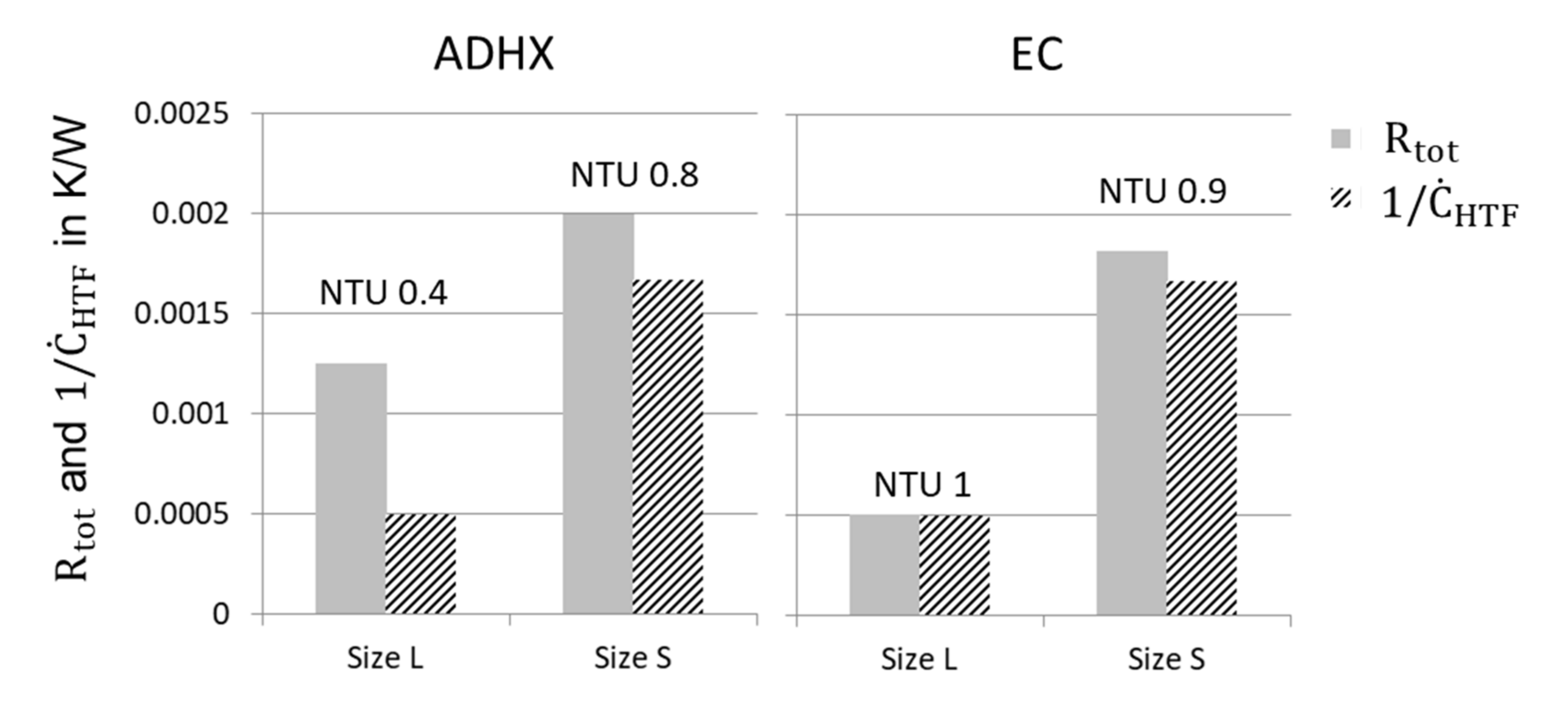
• Besides the heat and mass transfer resistance also the mass flow rate of the HTF is a relevant quantity which can limit the heat transfer within a component. Thus, the evaluation of the NTU and accordingly, the choice of the mass flow rate is decisive.

3. Results and Discussion

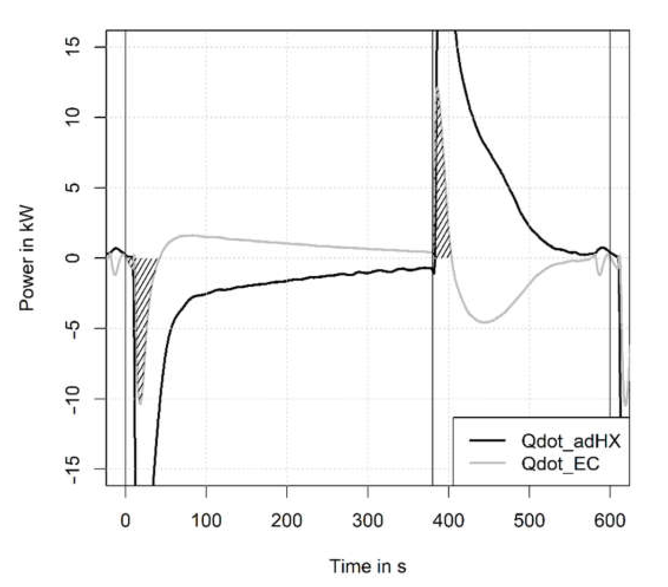
3.1. Temperature and Pressure Curves

Figure 6 shows typical temperature curves of the adsorption heat exchanger and the evaporator-condenser over a complete cycle. The valves are switched at 0 s, 380 s and 600 s as indicated by the black vertical lines. Since the volume flow rate is kept constant throughout the measurements, the evaporator-condenser is cooled down by the HTF at the beginning of the adsorption half cycle and is heated up by the HTF at the beginning of the desorption half cycle. This control strategy is different from the control strategy implemented by Wittstadt et al. [17]. In the measurements of Wittstadt et al. [17] the pump of the EC circuit is stopped after switching from evaporator to condenser and vice versa. In this case the evaporating working fluid cools the EC down to evaporator temperature or the condensing working fluid heats up the EC to condensing temperature when the half cycle is switched. Regarding the energy balance of the module, the two control strategies are the same. However, if the adsorption module is part of an adsorption heat pump, the control strategy as implemented by Wittstadt et al. [17] is preferable since it avoids transfer of heat into the low temperature source from the EC and it avoids transfer of heat from the middle temperature heat sink to the EC.

Figure 7 shows the pressure curve of the module and the calculated saturation pressure of the mean temperature of the HTF of the EC. The spike at t = 580 s is the pressure drop when the module is connected to the vacuum pump during the cycle as described in Section 2.1. As expected, the calculated saturation pressure of the EC mean temperature is above the module pressure during adsorption and below the module pressure during desorption.

With the volume flow rate and the temperature difference of the heat exchangers the power according to Equations (1) and (2) can be calculated. Figure 8 shows the resulting power curves. It is obvious that the desorption process ends after approximately 150 s—the measured power in both the adsorption heat exchanger and the EC drops below 200 W. The adsorption and the evaporation take much longer and would still go on if the adsorption half cycle time was longer. At the end of the adsorption half cycle the power of the EC is approximately 500 W in this case. Figure 9 shows the power curves of the adsorption half cycle for different half cycle times.

For the calculation of efficiency and power density the areas under the power curves are integrated. This integration yields the amount of energy during adsorption, desorption, evaporation, and condensation.

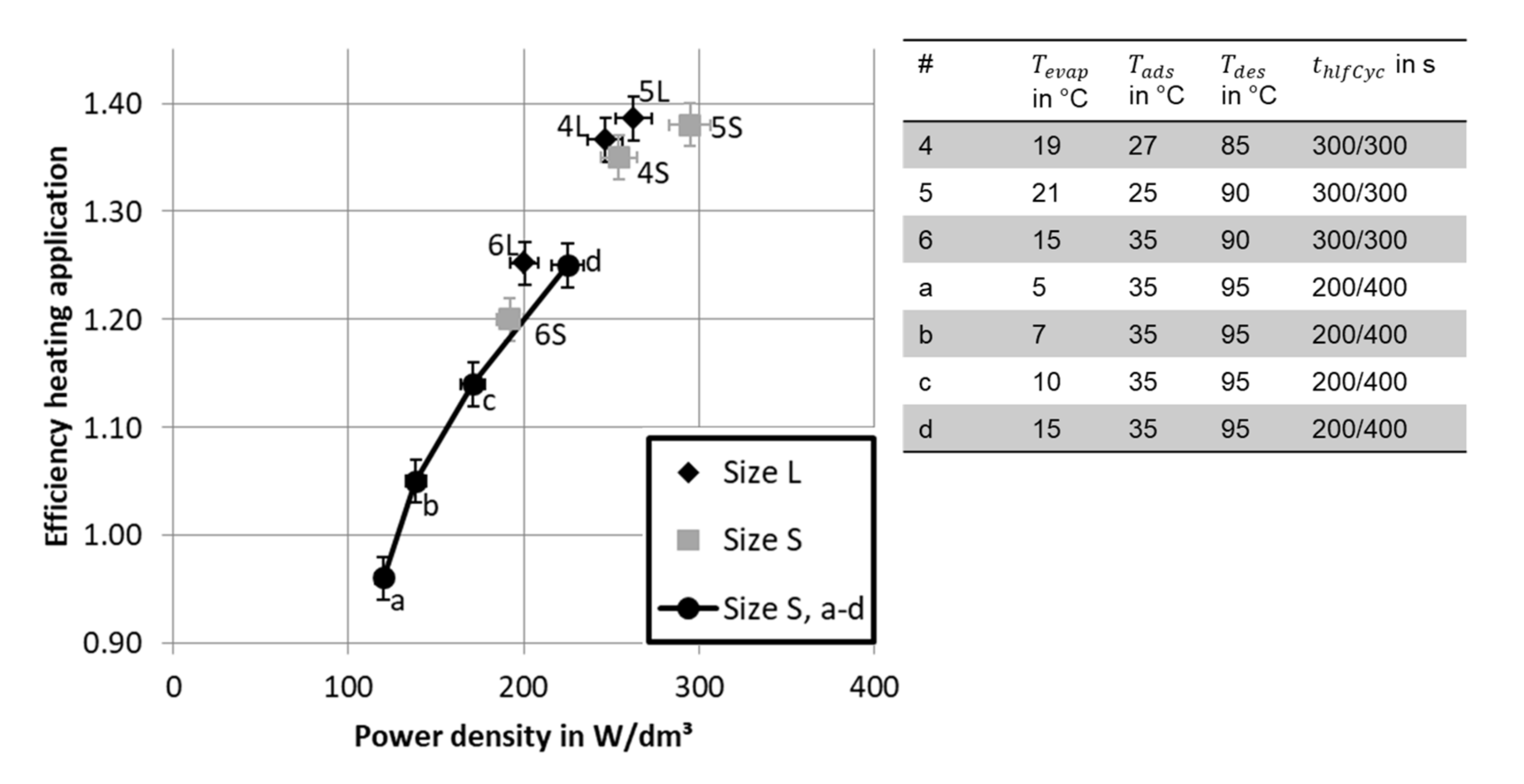
3.2. Efficiency and Power Density

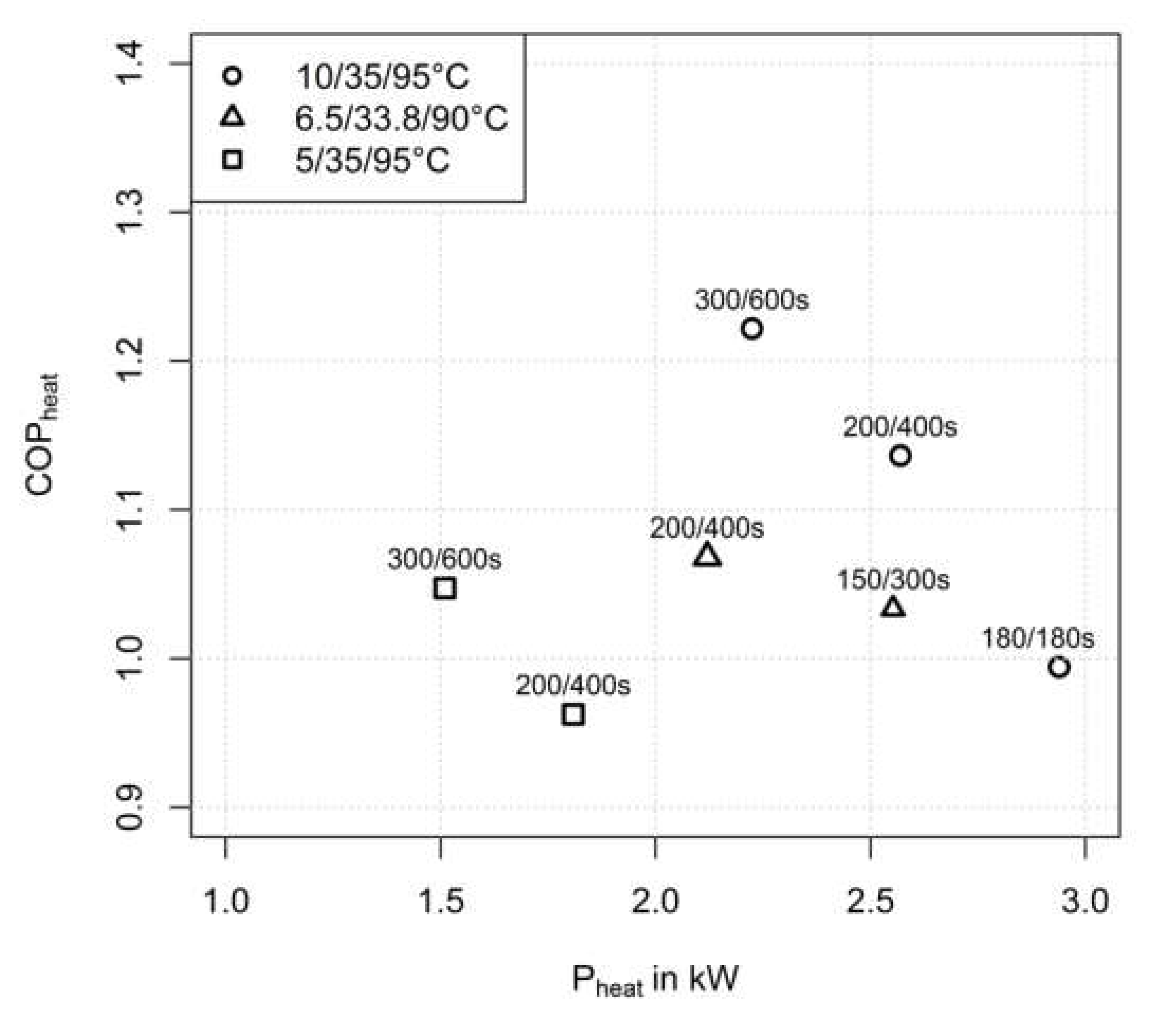
3.2.1. Influence of Half Cycle Time

Figure 10 shows the dependence of efficiency and power on the half cycle time for three different temperature conditions. As expected, the efficiency increases with the half cycle time and the power decreases with the half cycle time. For this kind of module and the temperature conditions we observed that the desorption (and condensation) is much faster than the adsorption (and evaporation) process. Thus, asymmetric half cycle times are chosen, i.e., the desorption half cycle is shorter than the adsorption half cycle. It can be seen that the operation window for an efficient cycle with reasonable output power is around 600 s total cycle time for the chosen temperature (and volume flow rate) conditions.

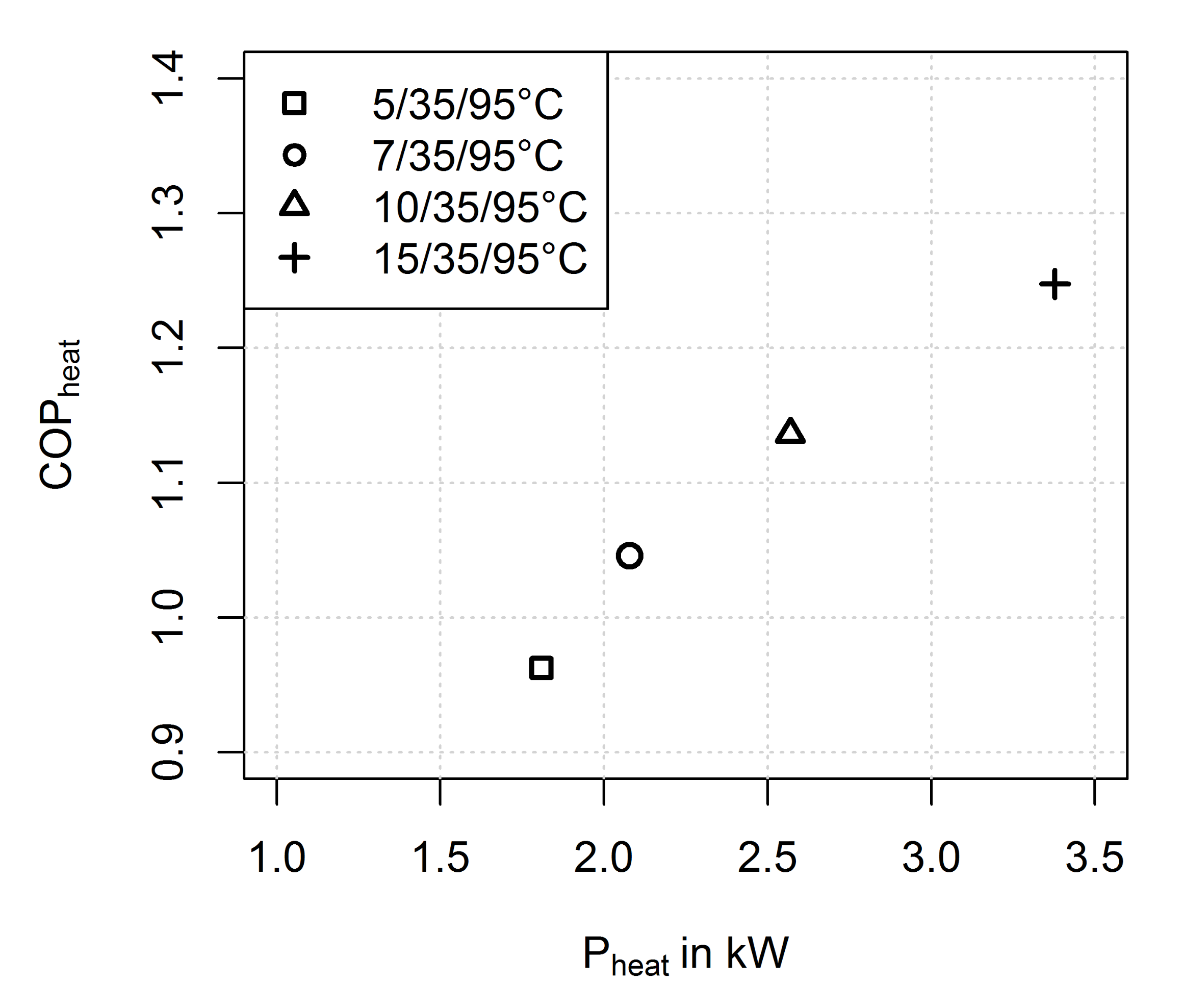
3.2.2. Influence of Evaporator Temperature

As shown in Figure 11, a decreasing evaporator temperature has a strong negative impact on the efficiency and power of the adsorption module. The efficiency drops from 1.28 to 0.98 and the power from 3.4 kW to 1.8 kW if the evaporator temperature is decreased from 15 °C to 5 °C.

The decreasing efficiency and power can partly be explained with the decreasing equilibrium loading difference (reached for very long cycle times) with decreasing evaporator temperature as shown in Figure 12. However, the calculated loading difference differs much more from the equilibrium loading difference for the measurement with 5 °C as for the measurement with 15 °C as shown in Figure 12.

Mainly there are two explanations for this observation:

• The heat and mass transfer resistance for adsorption and evaporation increases with a decreasing evaporator temperature (and thus, decreasing pressure of the water vapour)
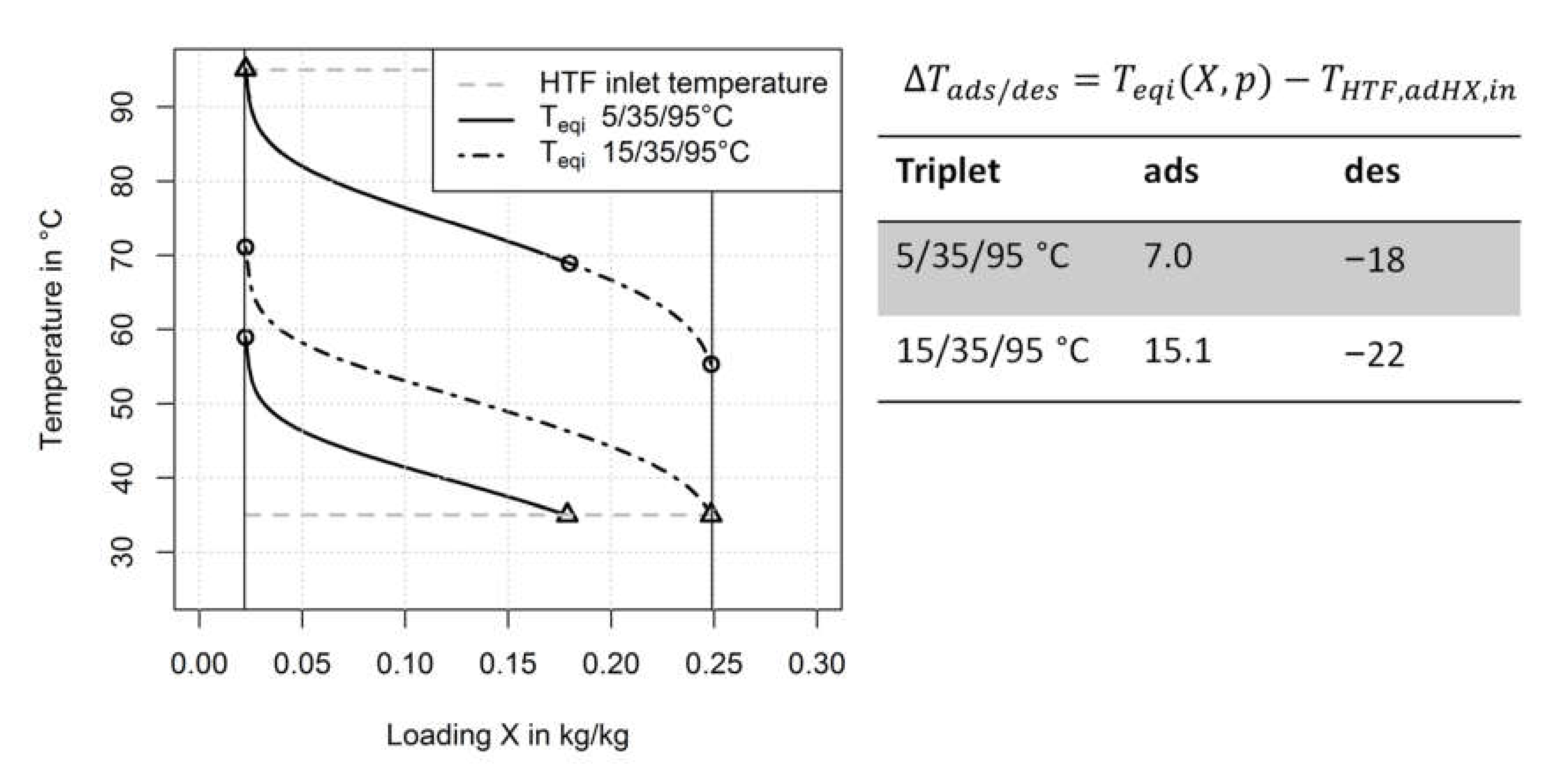
• The driving temperature differences for the heat and mass transfer processes decrease with decreasing evaporator temperature (and thus, decreasing pressure of the water vapour) as shown in Figure 13. If we compare the average values for the driving temperature differences in the adsorption half cycle it becomes clear that the loading difference of the 5/35/95 °C measurement can be at maximum half the loading difference of the 15/35/95 °C measurement.

Both explanations mentioned above will lead to a lower loading difference for same half cycle times. We will study the first explanation more in detail in Section 3.3.

Another factor that additionally lowers the efficiency is the increasing temperature difference between condensation and evaporation with a decreasing evaporator temperature. In case of a combined evaporator-condenser component the temperature change between evaporation and condensation detracts energy from the condensation half cycle. The higher the temperature difference between evaporation and condensation, the more energy from the condensation half cycle is consumed to change the temperature of the evaporator-condenser component.

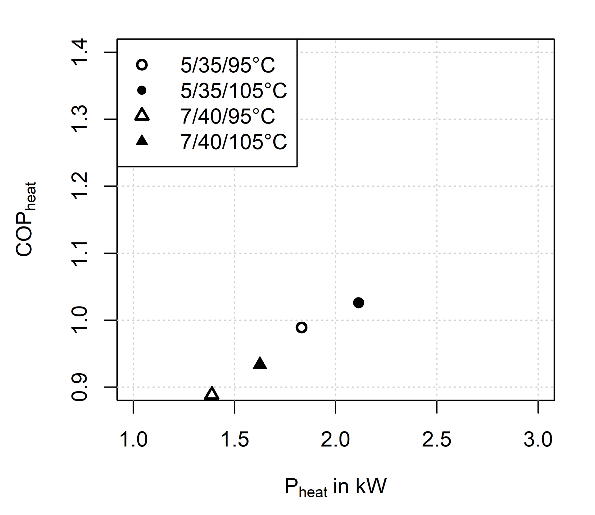
3.2.3. Influence of Adsorption/Condensation Temperature

We show in Figure 14 the results for measurements with different adsorption/condensation temperature ranging from 30 °C to 40 °C. It is obvious that 40 °C adsorption temperature is too high for the SAPO-34 / water pair at evaporation temperatures <10 °C—the efficiency is far below 1 for 7/40/95 °C or slightly above 1 with a slightly higher evaporation temperature of 10 °C.

3.2.4. Influence of Driving Temperature

We also studied the impact of the driving temperature on efficiency and power. The results are shown in Figure 15. An elevated driving temperature can improve the efficiency between 0.03 and 0.04 in absolute numbers. This was expected from the equilibrium data—the difference in the lower loading region that can be achieved with an elevated driving temperature is not that high (max. 0.015 kg/kg), consequently the improvement in terms of efficiency is not that high either.

3.3. Performance Evaluation of the Module

3.3.1. Heat and Mass Transfer Resistances

We evaluated the heat and mass transfer resistances as described in Section 2.5. The time-dependent curves are shown for a measurement in Figure 16 (left). First, the heat and mass transfer resistances during adsorption/evaporation half cycle are much higher than during the desorption/condensation half cycle. Secondly, during the switching phases the evaluation of heat and mass transfer resistances leads to values that are not meaningful. Third, the heat and mass transfer resistance is low at the beginning of the adsorption/evaporation half cycle and increases as adsorption and evaporation processes continue. This increase of the heat and mass transfer resistance might be an effect of increasing lengths of heat and mass transfer paths. However, with the available measured signals this hypothesis is rather speculative on this coarse level of evaluation and has to be verified or falsified for example with measurements on smaller structures.

For further evaluation we made a boxplot of the time-dependent heat and mass transfer resistances of the adsorption / evaporation half cycle. The results are shown in Figure 16 (right). It can be stated that the heat and mass transfer resistance of the adsorption heat exchanger does not obviously vary with the evaporator temperature. The heat and mass transfer resistance of this component is around 3 ± 0.5 × 10⁻³ K/W. In case of the evaporator-condenser component the heat and mass transfer resistance decreases from approximately 3.5 × 10⁻³ K/W to 2.5 × 10⁻³ K/W with an increase in the evaporator temperature from 5 °C to 10…15 °C. In conjunction with the much lower driving temperature difference as discussed in Section 3.2.2. and shown in Figure 13 it is obvious that the efficiency and power density of measurement ‘a’ must be much lower than the values of measurement ‘d’.

In order to check if the values for the heat and mass transfer resistances are plausible, we provide some data on the thermal resistance in the following. Based on the geometric data provided in Table 1 and Table 2 the necessary parameters for the calculation of the heat transfer resistance of the adsorption heat exchanger are listed in

Table 4. Calculation of the overall heat transfer resistance of the adsorption heat exchanger.

Parameter		Unit	Equation		Value
Heat transfer coefficient HTF-metal *1	${\alpha }_{HTF,mt}$	W/(m2K)	-	-	6000…7500
Heat conductance HTF-metal	${\left(UA\right)}_{HTF,mt}$	W/K	${\alpha }_{HTF,mt}\cdot A_{int,tb}$,	(11)	7000…8800
Heat conductivity fibrous structure	${\lambda }_{cmp}$	W/(m∙K)	-	-	5…8 *2
Heat conductance fibrous structure *3	${\left(UA\right)}_{\lambda ,cmp}$	W/K	$\frac{{\lambda }_{cmp}}{\frac{1}{3}\cdot \frac{1}{2}\cdot d_{cmp}}\cdot A_{tb,cmp},$	(12)	1900…3100
Overall heat transfer resistance	$R_{htTrn}$	10−3 K/W	$\frac{1}{{\left(UA\right)}_{HTF,mt}}+\frac{1}{{\left(UA\right)}_{\lambda ,cmp}}.$	(13)	0.47…0.67

*¹ calculated with offset strip fin correlation according to Shah and Sekulić [25] for temperature range 30…90 °C and mass flow rate of 0.167 kg./s. *² According to Fink et al. [35] it is rather 5 W/(m∙K), Velte [18] identified a value of around 8 W/(m∙K) with simulations of the ‘Size L’ module measurements. *³ The factor of 1/3 is due to the volumetric heat source term of adsorption according to Schwamberger [36] and Velte [18], the factor 1/2 is due to the geometry (1 fibrous structure in contact with 2 flat tubes).

. In this calculation of the overall heat transfer resistance, we neglect the conductive heat transfer resistance of the adsorbent layer and assume an ideal contact between fibrous structures and flat tubes.

The calculated overall heat transfer resistance of approximately 0.57 × 10⁻³ K/W for the adsorption heat exchanger is in the range of the values calculated from the measurement data in the desorption half cycle as shown in Figure 16 (left, ‘ADHX’). Furthermore, it is not too far away from the 0.42 × 10⁻³ K/W that Joos [30] determined with various temperature swing measurements on the module without working fluid (no ad- or desorption). Thus, the heat and mass transfer resistances calculated from the measurement have plausible values if we assume that there is no significant mass transfer resistance in the desorption half cycle. Compared to the heat and mass transfer resistance in the adsorption half cycle of 3 × 10⁻³ K/W, in the adsorption half cycle the mass transfer seems to limit the process.

We performed a similar calculation for the evaporator-condenser as listed in

Table 5. Calculation of the overall heat transfer resistance of the evaporator-condenser. We give two sets of values—evaporation (evap) and condensation (cond).

Parameter		Unit	Equation		Value Evap	Value Cond
Heat transfer coefficient HTF-metal *1	${\alpha }_{HTF,mt}$	W/(m2K)	-	-	6000	7500
Heat conductance HTF-metal	${\left(UA\right)}_{HTF,mt}$	W/K	${\alpha }_{HTF,mt}\cdot A_{int,tb},$	(14)	3500	4300
Heat conductivity fibrous structure	${\lambda }_{fib}$	W/(m∙K)	-	-	5…8 *2
Mean path length heat transfer	$l_{htTrn}$	mm	-	-	1…3	1.7
Ratio of wetted area	$f_{wet}$	1	-		1…0.1	1
Heat conductance fibrous structure	${\left(UA\right)}_{\lambda ,fib}$	W/K	$\frac{{\lambda }_{fib}}{l_{htTrn}}\cdot A_{tb,fib}\cdot f_{wet},$	(15)	200… 5800	3500
Overall heat transfer resistance	$R_{htTrn}$	10−3 K/W	$\frac{1}{{\left(UA\right)}_{HTF,mt}}+\frac{1}{{\left(UA\right)}_{\lambda ,fib}}.$	(16)	0.4… 5.5	0.4… 0.5

*¹ calculated with offset strip fin correlation according to Shah and Sekulić [25] for temperatures 10 °C evaporation and 40 °C (condensation) and mass flow rate of 0.167 kg./s. *² According to Fink et al. [35] it is rather 5 W/(m∙K), Velte [18] identified a value of around 8 W/(m∙K) with simulations of the ‘Size L’ module measurements.

. For this component it is much more difficult to estimate a mean path length for heat transfer $l_{htTrn}$ in the fibrous structure since this value will change during the evaporation process—it is likely that the evaporation first happens from places near the flat tube and the mean path length for heat transfer will then increase. Furthermore, as the evaporation process progresses, some parts of the evaporator-condenser component will run dry. Thus, the primary area in contact with the working fluid will decrease during the evaporation process. This is reflected by the ratio of wetted area $f_{wet}$ in Equation (15). In our calculation we neglect the conductive heat transfer resistance of the working fluid layer and assume an ideal contact between fibrous structures and flat tubes.

The values given for condensation in Table 5 are in the range of the values that are calculated from the measurement data as shown in Figure 16 (left, desorption half cycle, ‘EC’). If we assume that there is no significant mass transfer resistance during condensation the values in Figure 16 are quite plausible. They also match with the value of 0.5 × 10⁻³ K/W that Joos [30] determined with various temperature swing measurements on the module without working fluid. The range for the overall heat transfer resistance during evaporation in Table 5 is quite large but it is in the range of the data calculated from the measurement data shown in Figure 16 (left, adsorption half cycle, ‘EC’). However, it could be that the overall heat transfer resistance is lower due to a better distribution of the working fluid or a shorter mean path length for heat transfer. In this case, we would assume that there is a significant mass transfer resistance that leads to the values shown in Figure 16 (left, adsorption half cycle, ‘EC’). As stated before, from the data available in Figure 16 and the underlying assumptions of the data in Table 5 we cannot differentiate between heat and mass transfer.

3.3.2. Comparison with Other Studies

The module presented here was measured under the same temperature conditions and half cycle times as done by Wittstadt et al. [17]. Figure 17 shows the results for efficiency and power density. It can be seen that the module presented here has a slight advantage in terms of power density in points 4 and 5. The results for the other temperature conditions (point 6) show a lower efficiency and lower power density.

If we compare the heat and mass transfer resistances of both modules in Figure 18 (left) we can see that the “Size L” module has much lower heat and mass transfer resistances than the “Size S” module in absolute numbers. This can be expected, since the “Size L” module has much larger components and a higher adsorbent mass than the “Size S” module. However, if we scale the heat and mass transfer resistance with the component volume it can be seen in Figure 18 (right) that the components in both modules have nearly the same performance. It should be noted that the heat and mass transfer resistances for the “Size S” module differ from the values given in Figure 16 (point ‘d’) although the temperature boundary conditions are nearly the same. These higher resistances in Figure 16, which are approximately 3.2 × 10⁻³ K/W for adsorption and 2.5 × 10⁻³ K/W for evaporation, can be explained with the different half cycle times: the longer the half cycle time in adsorption the higher the heat and mass transfer resistance will be as it can be seen in Figure 16 (left).

In order to make the comparison complete, we include also the capacity flow of the heat transfer fluid in the evaluation as shown in Figure 19. Here we can see that the NTU figures of the evaporator-condenser component of ‘Size L’ and ‘Size S’ module are nearly the same. This is not the case for the adsorption—here the NTU of ‘Size L’ adsorption heat exchanger is only half as high as the related figure of the ‘Size S’ component. This means that the ‘Size S’ adsorption heat exchanger would require a higher mass flow rate of the HTF to make the efficiency and power density values comparable on the same basis. This is an interesting finding that we couldn’t include in the measurement campaign, but it should be included in future plans for module design and measurement planning.

3.4. Reproducibility

Measurements under the same temperature conditions (10/35/95 °C) and half cycle times (180/180 s) were conducted frequently as listed in

Table 6. Reproducibility of integral data.

No.	Date	COPheat	Pheat in kW	Comment
1	06.06.2019	1.02+/−0.01	2.9	Original measurement
2	20.01.2020	1.02+/−0.01	2.9	Reproducibility after 6 months (few other measurements during this period)
3	22.01.2020	1.02+/−0.01	3.0	Increased the filling level (+150 g)
4	04.02.2020	1.02+/−0.01	3.0	Final check of reproducibility

to ensure the reproducibility of the results.

The dynamic deviations of the signals are listed in

Table 7. Reproducibility of dynamic data in terms of root mean square deviation (RMSD).

No.	Date	RMSD(TEC) in K		RMSD(TADHX) in K		RMSD pmod in mbar
		in	out	in	out
1 → 2	20.01.2020	1	0.6	1.9	0.9	1.4
1 → 3	22.01.2020	0.7	0.5	0.9	0.8	1.2
1 → 4	04.02.2020	1.0	0.6	1.9	1.0	1.3

. The reference measurement is No. 1 in Table 6.

The integral data and the dynamic data show a quite good reproducibility despite the influence of the hydrogen formation and associated corrosion problem of the evaporator-condenser. The deviation of the dynamic data is mainly due to changes in the inlet temperature signal that depends on parameters of the test rig control that could not exactly be reproduced. Keeping in mind the corrosion problems it is remarkable that even after 6 months the module seems to be unchanged, and the original measurement could be reproduced.

4. Conclusions

We presented experimental data of an adsorption module with sintered aluminium fiber heat exchangers. The experimental data allows the study of the influence of half cycle time, evaporator temperature, adsorption/condensation temperature, and driving temperature on the efficiency and power density of the adsorption module. The evaluation of heat and mass transfer resistances reveals that the components of the adsorption module presented here (Size S) have the same volume scaled heat and mass transfer resistance as the adsorption module (Size L) presented by Wittstadt et al. [17]. This proves the scalability of the sintered aluminium fiber heat exchanger technology—it is possible to tailor the size of the adsorption module to achieve the desired average thermal power output with a moderate price in terms of additional thermal capacity of the ‘Size S’ module. The downsizing of the evaporator in the ‘Size S’ module has the effect of an increased heat and mass transfer resistance in the evaporation phase which is the limiting factor of this module. In case of the ‘Size L’ module the heat and mass transfer within the adsorption heat exchanger was the limiting factor. Furthermore, our results including two adsorption modules with different sized components demonstrate the applicability of the concept of using volume scaled heat and mass transfer resistances for the design of adsorption modules.

Another limiting factor of the ‘Size S’ module is the mass flow rate through the adsorption heat exchanger which should have been at least twice of the mass flow rate we chose in the experiments. This is an important finding which we will include in our considerations in future measurement campaigns. Relating the overall heat and mass transfer resistance of an adsorption heat exchanger to the capacity flow rate is an entirely new approach in literature and is the foundation of applying powerful methods of basic heat exchanger theory to adsorption heat exchangers.

References

1. Kemna, R.; van Elburg, M.; Corso, A.; Vigand, J.; Maagoe, V. Space and Combination Heaters—Market Analysis: Ecodesign and Energy Labelling; European Commision: Brussels, Belgium, 2019. [Google Scholar]
2. Pinheiro, J.M.; Salústio, S.; Rocha, J.; Valente, A.A.; Silva, C.M. Adsorption heat pumps for heating applications. Renew. Sustain. Energy Rev. 2020, 119, 109528. [Google Scholar] [CrossRef]
3. Dawoud, B. On the development of an innovative gas-fired heating appliance based on a zeolite-water adsorption heat pump; system description and seasonal gas utilization efficiency. Appl. Therm. Eng. 2014, 72, 323–330. [Google Scholar] [CrossRef]
4. Kühn, A. (Ed.) Thermally Driven Heat Pumps for Heating and Cooling; Universitätsverlag der TU Berlin: Berlin, Germany, 2013; ISBN 978-3-7983-2596-8. [Google Scholar]
5. Rivero-Pacho, A.M.; Critoph, R.E.; Metcalf, S.J. Modelling and development of a generator for a domestic gas-fired carbon-ammonia adsorption heat pump. Renew. Energy 2017, 110, 180–185. [Google Scholar] [CrossRef] [Green Version]
6. Metcalf, S.J.; Critoph, R.E.; Tamainot-Telto, Z. Optimal cycle selection in carbon-ammonia adsorption cycles. Int. J. Refrig. 2012, 35, 571–580. [Google Scholar] [CrossRef]
7. Mikhaeil, M.; Gaderer, M.; Dawoud, B. On the development of an innovative adsorber plate heat exchanger for adsorption heat transformation processes; An experimental and numerical study. Energy 2020, 207, 118272. [Google Scholar] [CrossRef]
8. Saleh, M.M.; AL-Dadah, R.; Mahmoud, S.; Elsayed, E.; El-Samni, O. Wire fin heat exchanger using aluminium fumarate for adsorption heat pumps. Appl. Therm. Eng. 2020, 164, 114426. [Google Scholar] [CrossRef]
9. Seol, S.-H.; Nagano, K.; Togawa, J. Modeling of adsorption heat pump system based on experimental estimation of heat and mass transfer coefficients. Appl. Therm. Eng. 2020, 171, 115089. [Google Scholar] [CrossRef]
10. Bendix, P.; Füldner, G.; Möllers, M.; Kummer, H.; Schnabel, L.; Henninger, S.; Henning, H.-M. Optimization of power density and metal-to-adsorbent weight ratio in coated adsorbers for adsorptive heat transformation applications. Appl. Therm. Eng. 2017, 124, 83–90. [Google Scholar] [CrossRef]
11. Mohammadzadeh Kowsari, M.; Niazmand, H.; Tokarev, M.M. Bed configuration effects on the finned flat-tube adsorption heat exchanger performance: Numerical modeling and experimental validation. Appl. Energy 2018, 213, 540–554. [Google Scholar] [CrossRef]
12. Calabrese, L.; Bruzzaniti, P.; Palamara, D.; Freni, A.; Proverbio, E. New SAPO-34-SPEEK composite coatings for adsorption heat pumps: Adsorption performance and thermodynamic analysis. Energy 2020, 203, 117814. [Google Scholar] [CrossRef]
13. Hinze, M.; Ranft, F.; Drummer, D.; Schwieger, W. Reduction of the heat capacity in low-temperature adsorption chillers using thermally conductive polymers as heat exchangers material. Energy Convers. Manag. 2017, 145, 378–385. [Google Scholar] [CrossRef]
14. Schnabel, L.; Füldner, G.; Velte, A.; Laurenz, E.; Bendix, P.; Kummer, H.; Wittstadt, U. Innovative Adsorbent Heat Exchangers: Design and Evaluation. In Innovative Heat Exchangers; Bart, H.-J., Scholl, S., Eds.; Springer: Cham, Switzerland, 2018; pp. 363–394. ISBN 978-3-319-71641-1. [Google Scholar]
15. Caprì, A.; Frazzica, A.; Calabrese, L. Recent Developments in Coating Technologies for Adsorption Heat Pumps: A Review. Coatings 2020, 10, 855. [Google Scholar] [CrossRef]
16. Wittstadt, U.; Füldner, G.; Andersen, O.; Herrmann, R.; Schmidt, F. A New Adsorbent Composite Material Based on Metal Fiber Technology and Its Application in Adsorption Heat Exchangers. Energies 2015, 8, 8431–8446. [Google Scholar] [CrossRef]
17. Wittstadt, U.; Füldner, G.; Laurenz, E.; Warlo, A.; Große, A.; Herrmann, R.; Schnabel, L.; Mittelbach, W. A novel adsorption module with fiber heat exchangers: Performance analysis based on driving temperature differences. Renew. Energy 2017, 110, 154–161. [Google Scholar] [CrossRef]
18. Velte, A. Experimentelle Arbeiten und Entwicklung von numerischen Modellen zur Analyse und Optimierung von Erweiterten Adsorptionskreisläufen für die Wärmeversorgung von Gebäuden. Ph.D. Thesis, Albert-Ludwigs-Universität Freiburg, Freiburg, Germany, 2018. [Google Scholar]
19. Bauer, J.; Herrmann, R.; Mittelbach, W.; Schwieger, W. Zeolite/aluminum composite adsorbents for application in adsorption refrigeration. Int. J. Energy Res. 2009, 33, 1233–1249. [Google Scholar] [CrossRef]
20. Wittstadt, U.; Laurenz, E.; Velte, A.; Füldner, G. Using Driving Temperature Difference Equivalents to Compare Heat and Mass Transport Limitations in Sorption Modules and Adsorption Heat Exchangers: Poster at the Sorption Friends Conference, Milazzo, Italy, 14–16 September 2015. Available online: http://www.sorptionfriends.org/poster/ (accessed on 24 April 2017).
21. Velte, A.; Herrmann, R.; Andersen, O.; Wittstadt, U.; Füldner, G.; Schnabel, L. Experimental Characterization of Aluminum Fibre/SAPO-34 Composites for Adsorption Heat Pump Applications. In Proceedings of the Heat Powered Cycles, Nottingham, UK, 26–29 June 2016. [Google Scholar]
22. Wittstadt, U. Experimentelle und Modellgestützte Charakterisierung von Adsorptionswärmeübertragern. Ph.D. Thesis, Technische Universität Berlin, Berlin, Germany, 2018. [Google Scholar]
23. Ammann, J.; Ruch, P.; Michel, B.; Studart, A.R. Quantification of heat and mass transport limitations in adsorption heat exchangers: Application to the silica gel/water working pair. Int. J. Heat Mass Transf. 2018, 123, 331–341. [Google Scholar] [CrossRef]
24. Ammann, J.; Michel, B.; Ruch, P.W. Characterization of transport limitations in SAPO-34 adsorbent coatings for adsorption heat pumps. Int. J. Heat Mass Transf. 2019, 129, 18–27. [Google Scholar] [CrossRef]
25. Shah, R.K.; Sekulić, D.P. Fundamentals of Heat Exchanger Design; Wiley-Interscience: Hoboken, NJ, USA, 2003; ISBN 0-471-32171-0. [Google Scholar]
26. Baehr, H.D.; Stephan, K. Wärme- und Stoffübertragung; 6, bearb. Aufl.; Springer Berlin: Berlin, Germany, 2008; ISBN 978-3-540-87688-5. [Google Scholar]
27. Miyazaki, T.; Akisawa, A. The influence of heat exchanger parameters on the optimum cycle time of adsorption chillers. Appl. Therm. Eng. 2009, 29, 2708–2717. [Google Scholar] [CrossRef]
28. Velte, A.; Joos, L.; Kostmann, C.; Fink, M.; Füldner, G. Experimental investigation of an adsorption module based on heat exchangers with fibrous aluminium structures and the SAPO-34/water working pair for gas-driven adsorption heat pumps. In Proceedings of the ISHPC 2021 Proceedings, Online Pre-Conference 2020, Berlin, Germany, 22–25 August 2021; Meyer, T., Ed.; Technische Universität Berlin: Berlin, Germany, 2020. [Google Scholar]
29. Gluesenkamp, K.R.; Frazzica, A.; Velte, A.; Metcalf, S.; Yang, Z.; Rouhani, M.; Blackman, C.; Qu, M.; Laurenz, E.; Rivero-Pacho, A.; et al. Experimentally Measured Thermal Masses of Adsorption Heat Exchangers. Energies 2020, 13, 1150. [Google Scholar] [CrossRef] [Green Version]
30. Joos, L. Vermessung von Adsorptionsmodulen und Charakterisierung Mittels Dynamischer Simulationen. Master’s Thesis, Technische Universität Berlin, Berlin, Germany, 2019. [Google Scholar]
31. Desai, A.; Schwamberger, V.; Herzog, T.; Jänchen, J.; Schmidt, F.P. Modeling of Adsorption Equilibria through Gaussian Process Regression of Data in Dubinin’s Representation: Application to Water/Zeolite Li-LSX. Ind. Eng. Chem. Res. 2019, 58, 17549–17554. [Google Scholar] [CrossRef]
32. Wagner, W.; Cooper, J.R.; Dittmann, A.; Kijima, J.; Kretzschmar, H.-J.; Kruse, A.; Mares, R.; Oguchi, K.; Sato, H.; Stöcker, I.; et al. The IAPWS Industrial Formulation 1997 for the Thermodynamic Properties of Water and Steam. J. Eng. Gas Turbines Power 2000, 122, 150–184. [Google Scholar] [CrossRef]
33. Holmgren, M. XSteam. Available online: https://www.academia.edu/download/39720574/X_Steam_for_Matlab.pdf (accessed on 10 March 2020).
34. Lanzerath, F.; Bau, U.; Seiler, J.; Bardow, A. Optimal design of adsorption chillers based on a validated dynamic object-oriented model. Sci. Technol. Built Environ. 2015, 21, 248–257. [Google Scholar] [CrossRef] [Green Version]
35. Fink, M.; Andersen, O.; Seidel, T.; Schlott, A. Strongly Orthotropic Open Cell Porous Metal Structures for Heat Transfer Applications. Metals 2018, 8, 554. [Google Scholar] [CrossRef] [Green Version]
36. Schwamberger, V. Thermodynamische und Numerische Untersuchung Eines Neuartigen Sorptionszyklus zur Anwendung in Adsorptionswärmepumpen und -kältemaschinen = Thermodynamic and Numerical Investigation of a Novel Sorption Cycle for Application in Adsorption Heat Pumps and Chillers. Ph.D. Thesis, Karlsruher Institut für Technologie, Karlsruher, Germany, 2016. [Google Scholar]
Figure 1. Thermal capacities of the sorption modules (left), picture of the module ‘Size S’ (middle) [30], detail of the fiber heat exchanger (right) [30].
Energies 15 02823 g001
Figure 2. Measured adsorption equilibrium data in Dubinin’s representation (grey circles: measured pressure p, temperature T, and loading X transformed into specific adsorbed volume W and adsorption potential A) and Gaussian Process (GP) Regression of the dataset (black line).
Energies 15 02823 g002
Figure 3. Schematic drawing of the test rig at Fraunhofer ISE [30] with its three temperature level tanks (HT high temperature, MT medium temperature, LT low temperature). The four inlet and outlet temperatures are measured in closest proximity to the adsorption module to avoid a bias due to the thermal capacity of the HTF between adsorption module and temperature sensor. The large volume of the tanks (500 dm3 each) helps to achieve sharp temperature profiles.
Energies 15 02823 g003
Figure 4. Test rig at Fraunhofer ISE with its three temperature level tanks (HT high temperature, MT medium temperature, LT low temperature), the mixing unit, and an adsorption module. The position of the volume flow rate sensors is additionally indicated. The temperature of the HTF is measured in closest proximity at the inlets and outlets of the adsorption module.
Energies 15 02823 g004
Figure 5. Above: Simple driving temperature difference model with one single resistance, middle: Driving temperature difference model with a heat- and a mass transfer resistance and a thermal capacitance, below: Heat and mass transfer resistance model for adsorption heat exchanger and combined evaporator-condenser. We measure the yellow marked state variables with our test rig.
Energies 15 02823 g005
Figure 6. Temperature curves of the adsorption heat exchanger in/out and evaporator/condenser in/out. Temperature boundary conditions are 10/35/95 °C, 400 s adsorption, 200 s desorption half cycle time, volume flow rate is kept constant at 10 L/min for each heat exchanger throughout the whole measurement.
Energies 15 02823 g006
Figure 7. Pressure curves of module and calculated saturation pressure of the evaporator/condenser mean temperature. Temperature boundary conditions are 10/35/95 °C, 400 s adsorption, 200 s desorption half cycle time, volume flow rate is kept constant at 10 L/min for each heat exchanger throughout the whole measurement.
Energies 15 02823 g007
Figure 8. Calculated power of adsorption heat exchanger and evaporator-condenser over a complete cycle. Temperature boundary conditions are 10/35/95 °C, 400 s adsorption, 200 s desorption half cycle time, volume flow rate is kept constant at 10 l/min for each heat exchanger throughout the whole measurement. The two shaded areas under the power curve of the EC during the switching phase indicate the cooling down and the heating up of the evaporator-condenser. The error bars are below the thickness of the plotted lines.
Energies 15 02823 g008
Figure 9. Calculated power of adsorption heat exchanger and evaporator-condenser over the adsorption half cycle for different half cycle times. Temperature boundary conditions are 10/35/95 °C, volume flow rate is kept constant at 10 l/min for each heat exchanger throughout the whole measurement. The two horizontal lines indicate −250 W and 250 W, respectively. The error bars are below the thickness of the plotted lines.
Energies 15 02823 g009
Figure 10. Efficiency and power for three different temperature conditions and different half cycle times. The half cycle times are given as desorption half cycle time followed by the adsorption half cycle time in the plot. The longer the half cycle time, the higher the efficiency due to the higher loading difference. Consequently, longer half cycle time corresponds with lower power.
Energies 15 02823 g010
Figure 11. Efficiency and power for four different temperature conditions. We conducted all measurements shown here with the same half cycle time (200 s/400 s for desorption/adsorption). Due to the rising evaporator temperature the maximum possible loading difference increases and the temperature lift (difference between evaporator temperature and adsorber temperature during adsorption) decreases. This corresponds with a higher efficiency as it can be expected from theory.
Energies 15 02823 g011
Figure 12. Loading difference calculated with the measured data compared to the loading difference that can be expected if sorption equilibrium is reached at the end of the adsorption and desorption half cycle. The loading differences are evaluated for the four different temperature conditions studied in this section.
Energies 15 02823 g012
Figure 13. Equilibrium temperature in adsorption and desorption plotted versus loading for two different temperature conditions. The starting points are marked with a circle ‘o’ and the ending points with a triangle ‘Δ’. The difference between the equilibrium temperature and the HTF temperature (here: inlet temperature) is the maximum driving temperature difference during adsorption or desorption. The table shows the average values of the driving temperature difference over the whole loading range.
Energies 15 02823 g013
Figure 14. Efficiency and power for different temperature conditions. We show a variation of the adsorption/condensation temperature from 30 °C to 40 °C for an evaporator temperature of 7 °C. Further, the impact of a slightly higher evaporator temperature (10 °C) is shown. We conducted all measurements shown here with the same half cycle time (200 s/400 s for desorption/adsorption).
Energies 15 02823 g014
Figure 15. Efficiency and power for 5/35 °C and 7/40 °C temperature conditions and two different driving temperatures (95 °C and 105 °C). A small improvement in terms of efficiency is possible with an elevated driving temperature.
Energies 15 02823 g015
Figure 16. Time-dependent curves for heat and mass transfer resistances for measurement “c” 10/35/95 °C, 200/400 s half cycle time (left), boxplot of heat and mass transfer resistances during adsorption/evaporation half cycle for measurements with different evaporator temperatures (right). The overall heat and mass transfer resistance of the ADHX is not affected by the different evaporator temperatures.
Energies 15 02823 g016
Figure 17. Efficiency and power density for the two different modules (Size S and Size L) for three different temperature conditions (points 4, 5, 6) and the data for Size S module for different evaporator temperatures as presented in Section 3.2.2.
Energies 15 02823 g017
Figure 18. Boxplot of heat and mass transfer resistances for measurements under 15/35/90 °C temperature conditions and 300 s half cycle time in absolute numbers (left) and volume scaled values (right). The component volume is plotted for convenience. The volume scaled overall heat and mass transfer resistance are nearly the same for ‘Size S’ and ‘Size L’ module.
Energies 15 02823 g018
Figure 19. Heat and mass transfer resistances for measurements under 15/35/90 °C temperature conditions and 300 s half cycle time. The reciprocal value of the capacity flow of the heat transfer fluid is additionally plotted for each component. The resulting NTU figure according to Equation (10) is also shown.
Energies 15 02823 g019