
Mechanistic Model of an Air Cushion Surge Tank for Hydro Power Plants


Abstract
:1. Introduction
1.1. Background
1.2. Previous Work and Contributions
- a mechanistic model of an ACST, and
- a comparison between the ACST models with and without air friction.
1.3. Outline
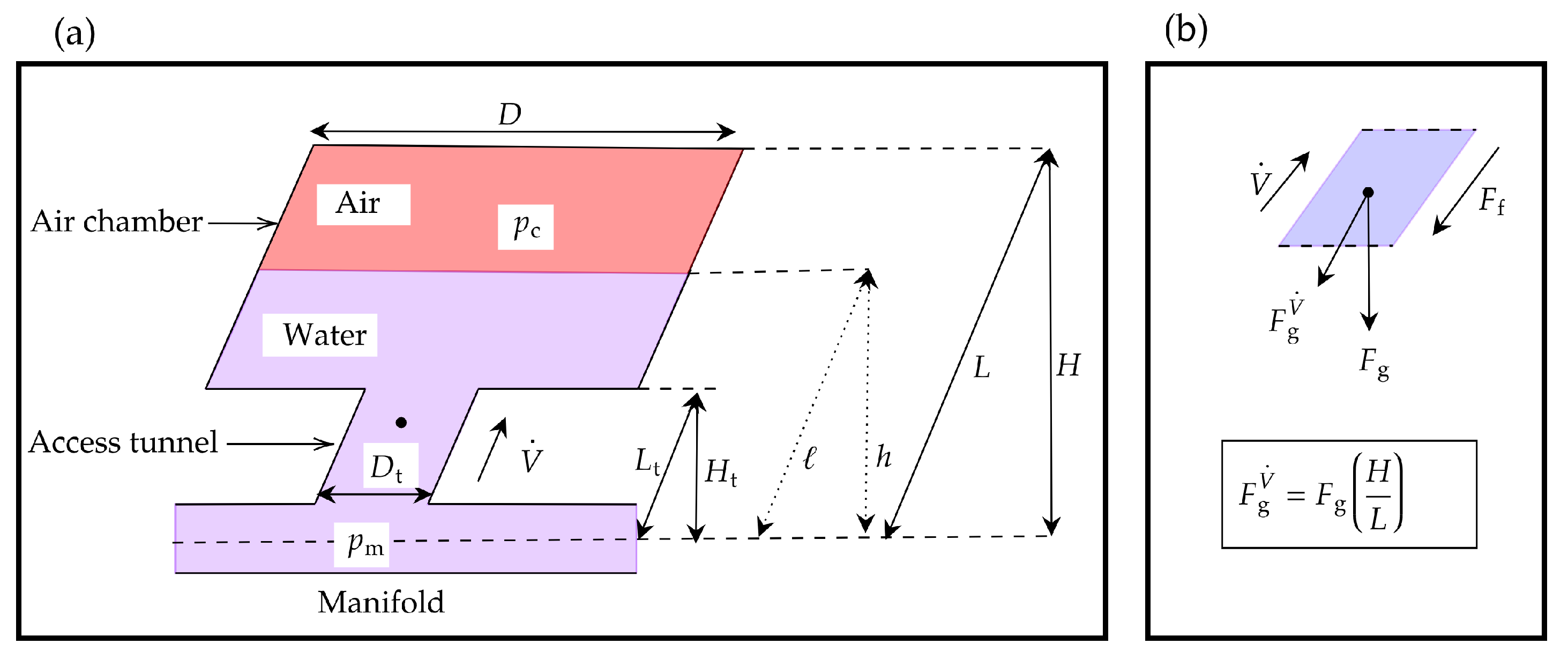
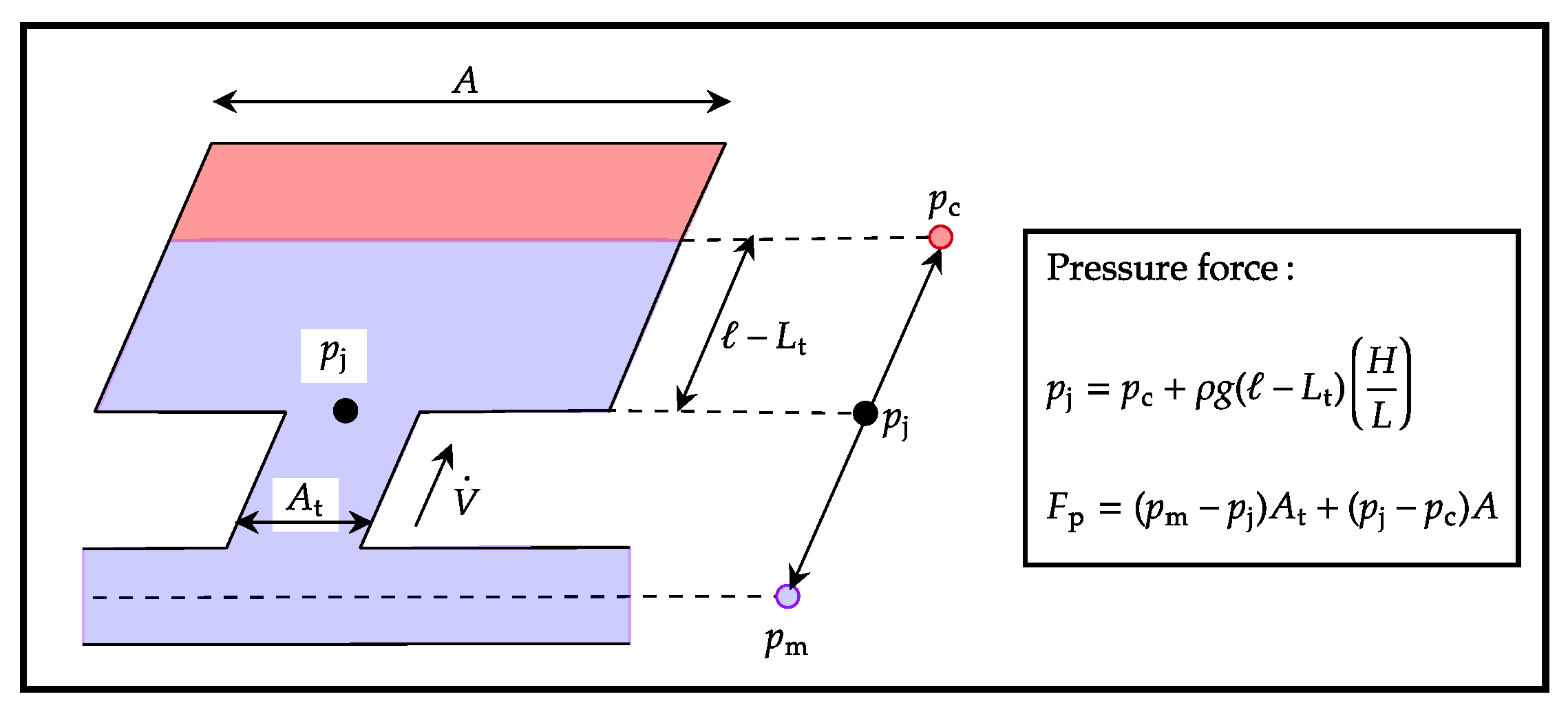
2. Mechanistic Model of ACST
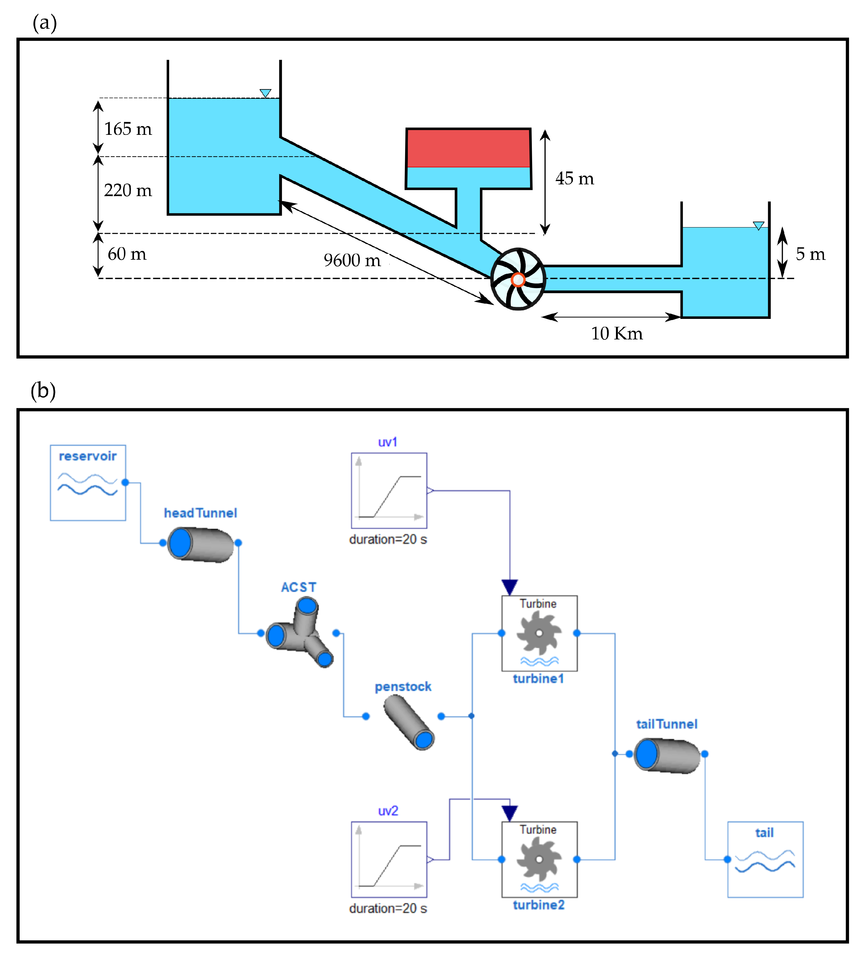
2.1. Case
2.2. Case
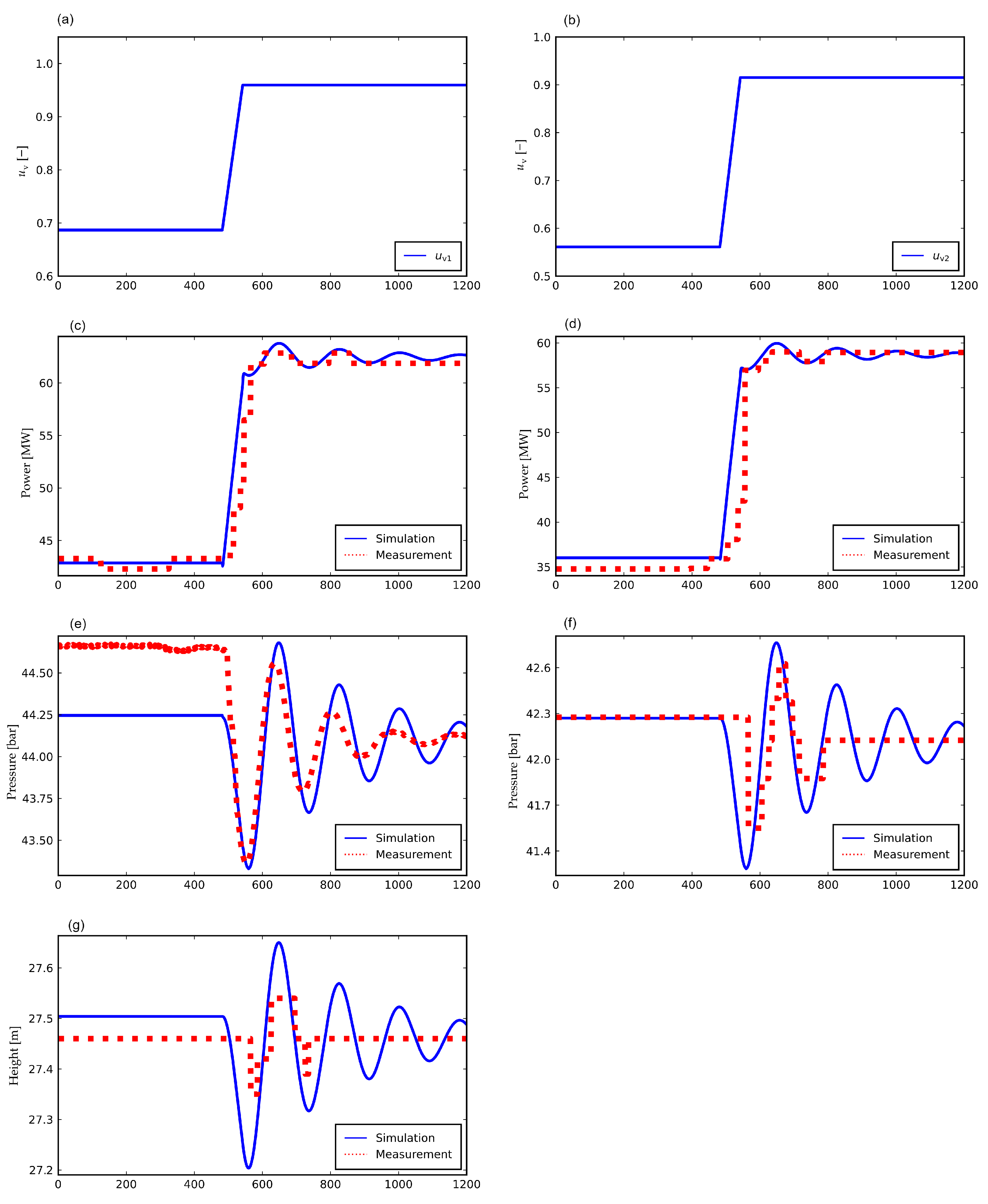
3. Case Study
- validate the model with the experimental data from [10],
- simulate the model considering air friction inside the ACST, and
- study the hydraulic behavior of the ACST at different load acceptances and rejections.
3.1. Simulation Versus Real Measurements
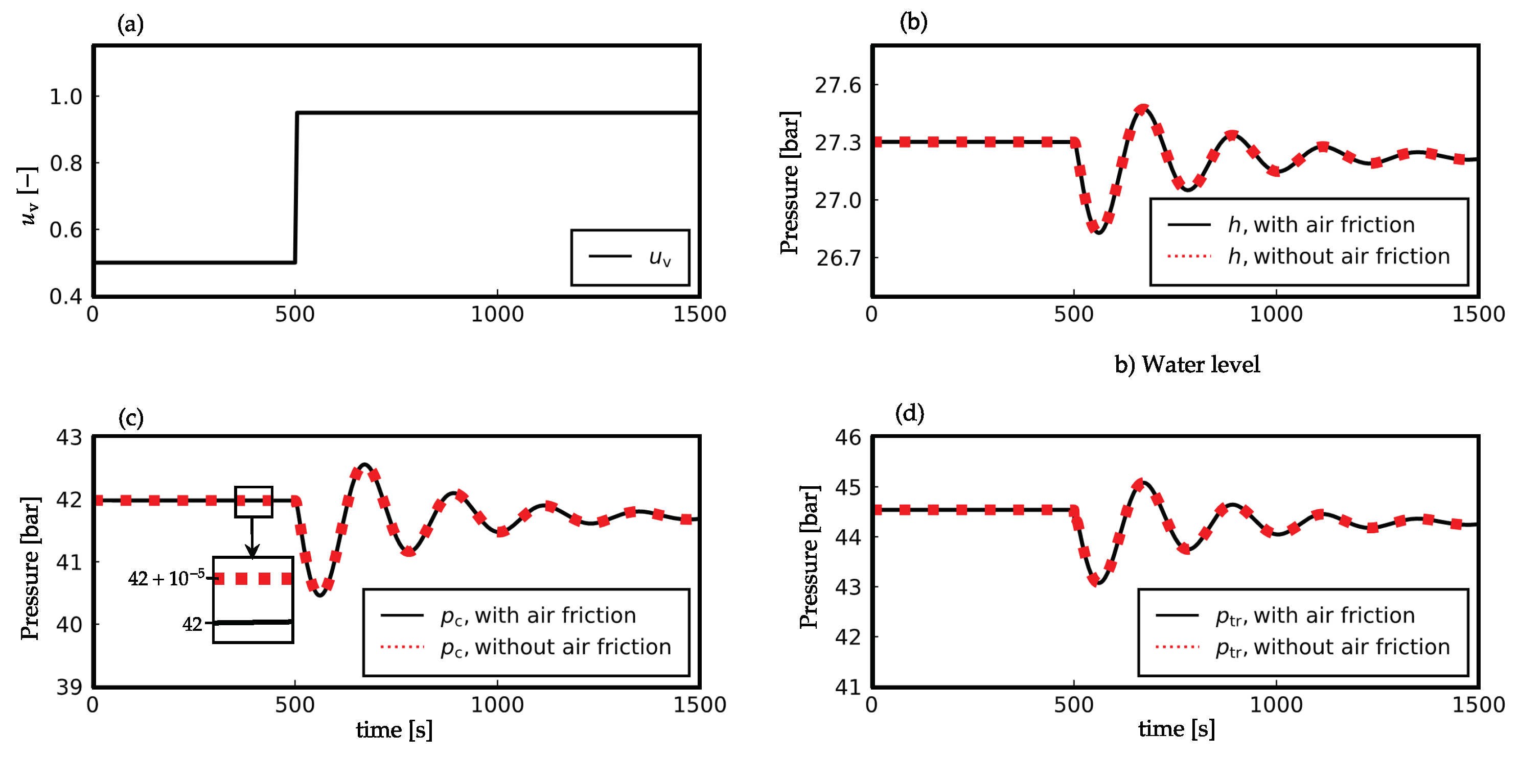
3.2. Effect of Air Friction Inside ACST
3.3. Operations of ACST in Load Acceptance and Rejection
3.3.1. Load Acceptances
3.3.2. Load Rejections
3.3.3. ACST as a Flexible Hydro Power
4. Conclusions and Future Work
Author Contributions
Funding
Institutional Review Board Statement
Informed Consent Statement
Data Availability Statement
Acknowledgments
Conflicts of Interest
References
- Pandey, M.; Winkler, D.; Sharma, R.; Lie, B. Using MPC to Balance Intermittent Wind and Solar Power with Hydro Power in Microgrids. Energies 2021, 14, 874. [Google Scholar] [CrossRef]
- Pandey, M.; Lie, B. The Role of Hydropower Simulation in Smart Energy Systems. In Proceedings of the 2020 IEEE 7th International Conference on Energy Smart Systems (ESS), Kyiv, Ukraine, 12–14 May 2020; pp. 392–397. [Google Scholar]
- Charmasson, J.; Belsnes, M.; Andersen, O.; Eloranta, A.; Graabak, I.; Korpås, M.; Helland, I.; Sundt, H.; Wolfgang, O. Roadmap for Large-Scale Balancing and Energy Storage from Norwegian Hydropower: Opportunities, Challanges and Needs until 2050; SINTEF Energi AS: Trondheim, Norway, 2018. [Google Scholar]
- Huertas-Hernando, D.; Farahmand, H.; Holttinen, H.; Kiviluoma, J.; Rinne, E.; Söder, L.; Milligan, M.; Ibanez, E.; Martínez, S.M.; Gomez-Lazaro, E.; et al. Hydro power flexibility for power systems with variable renewable energy sources: An IEA Task 25 collaboration. Wiley Interdiscip. Rev. Energy Environ. 2017, 6, e220. [Google Scholar] [CrossRef] [Green Version]
- Graabak, I.; Korpås, M.; Jaehnert, S.; Belsnes, M. Balancing future variable wind and solar power production in Central-West Europe with Norwegian hydropower. Energy 2019, 168, 870–882. [Google Scholar] [CrossRef]
- Pandey, M.; Lie, B. The influence of surge tanks on the water hammer effect at different hydro power discharge rates. In Proceedings of the SIMS 2020, Oulu, Finland, 22–24 September 2020; Linköping University Electronic Press: Linköping, Sweden, 2020; pp. 125–130. [Google Scholar]
- Vereide, K.; Richter, W.; Zenz, G.; Lia, L. Surge Tank Research in Austria and Norway. Wasserwirtschaft 2015, 1, 58–62. [Google Scholar] [CrossRef] [Green Version]
- Vereide, K.; Lia, L.; Nielsen, T. Physical modelling of hydropower waterway with air cushion surge chamber. In Proceedings of the 5th International Symposium on Hydraulic Structures, Brisbane, Australia, 25–27 June 2014. [Google Scholar]
- Pandey, M.; Lie, B. Mechanistic modeling of different types of surge tanks and draft tubes for hydropower plants. In Proceedings of the SIMS 2020, Oulu, Finland, 22–24 September 2020; Linköping University Electronic Press: Linköping, Sweden, 2020; pp. 131–138. [Google Scholar]
- Vereide, K.; Lia, L.; Nielsen, T.K. Hydraulic scale modelling and thermodynamics of mass oscillations in closed surge tanks. J. Hydraul. Res. 2015, 53, 519–524. [Google Scholar] [CrossRef] [Green Version]
- Mosonyi, E. Water Power Development: High-Head Power Plants; Akadémiai kiadó: Budapest, Hungary, 1965; Volume 2. [Google Scholar]
- Pickford, J. Analysis of Water Surge; Taylor & Francis: Abingdon, UK, 1969. [Google Scholar]
- Jaeger, C. Present trends in surge tank design. Proc. Inst. Mech. Eng. 1954, 168, 91–124. [Google Scholar] [CrossRef]
- Guo, J.; Woldeyesus, K.; Zhang, J.; Ju, X. Time evolution of water surface oscillations in surge tanks. J. Hydraul. Res. 2017, 55, 657–667. [Google Scholar] [CrossRef]
- Lydersen, A. Fluid Flow and Heat Transfer; John Wiley & Sons Incorporated: Hoboken, NJ, USA, 1979. [Google Scholar]
- Vereide, K.V. Hydraulics and Thermodynamics of Closed Surge Tanks for Hydropower Plants. Ph.D. Thesis, NTNU, Trondheim, Norway, 2016. [Google Scholar]
- Wang, C.; Yang, J.; Nilsson, H. Simulation of water level fluctuations in a hydraulic system using a coupled liquid-gas model. Water 2015, 7, 4446–4476. [Google Scholar] [CrossRef] [Green Version]
- Yulong, L. Studies on gas loss of air cushion surge chamber based on gas seepage theory. In Proceedings of the 2011 International Conference on Electric Technology and Civil Engineering (ICETCE), Lushan, China, 22–24 April 2011; pp. 723–725. [Google Scholar]
- Ou, C.; Liu, D.; Li, L. Research on dynamic properties of long pipeline monitoring system of air cushion surge chamber. In Proceedings of the 2009 Asia-Pacific Power and Energy Engineering Conference, Wuhan, China, 27–31 March 2009; pp. 1–4. [Google Scholar]
- Yang, X.L.; Kung, C.S. Stability of air-cushion surge tanks with throttling. J. Hydraul. Res. 1992, 30, 835–850. [Google Scholar] [CrossRef]
- Vytvytskyi, L. User’s Guide for the Open Hydropower Library (OpenHPL); University of South-Eastern Norway: Porsgrunn, Norway, 2019. [Google Scholar]
- Vytvytsky, L.; Lie, B. Comparison of elastic vs. inelastic penstock model using OpenModelica. In Proceedings of the 58th Conference on Simulation and Modelling (SIMS 58), Reykjavik, Iceland, 25–27 September 2017; Linköping University Electronic Press: Linköping, Sweden, 2017; Volume 138, pp. 20–28. [Google Scholar] [CrossRef] [Green Version]
- Vytvytskyi, L.; Lie, B. Mechanistic model for Francis turbines in OpenModelica. IFAC-PapersOnLine 2018, 51, 103–108. [Google Scholar] [CrossRef]
- Vereide, K.; Svingen, B.; Nielsen, T.K.; Lia, L. The effect of surge tank throttling on governor stability, power control, and hydraulic transients in hydropower plants. IEEE Trans. Energy Convers. 2016, 32, 91–98. [Google Scholar] [CrossRef] [Green Version]
- Rakhsha, M.; Kees, C.E.; Negrut, D. Lagrangian vs. Eulerian: An analysis of two solution methods for free-surface flows and fluid solid interaction problems. Fluids 2021, 6, 460. [Google Scholar] [CrossRef]
- Bimbato, A.M.; Alcântara Pereira, L.A.; Hirata, M.H. Study of surface roughness effect on a bluff body—The formation of asymmetric separation bubbles. Energies 2020, 13, 6094. [Google Scholar] [CrossRef]


| Quantity | Symbol | Value |
|---|---|---|
| Hydraulic diameter of the throat | ||
| Hydraulic diameter of the chamber | D | |
| Length of the throat | ||
| Total height | H | |
| Total length | L | |
| Pipe roughness height | ||
| Total volume | − | |
| Operating temperature | ||
| Adiabatic exponent for air at STP | ||
| Molar mass of air at STP | ||
| Universal gas constant | R | |
| Initial pressure of air | ||
| Initial water level | ||
| Initial volume of air |
Publisher’s Note: MDPI stays neutral with regard to jurisdictional claims in published maps and institutional affiliations. |
© 2022 by the authors. Licensee MDPI, Basel, Switzerland. This article is an open access article distributed under the terms and conditions of the Creative Commons Attribution (CC BY) license (https://creativecommons.org/licenses/by/4.0/).
Share and Cite
Pandey, M.; Winkler, D.; Vereide, K.; Sharma, R.; Lie, B. Mechanistic Model of an Air Cushion Surge Tank for Hydro Power Plants. Energies 2022, 15, 2824. https://doi.org/10.3390/en15082824
Pandey M, Winkler D, Vereide K, Sharma R, Lie B. Mechanistic Model of an Air Cushion Surge Tank for Hydro Power Plants. Energies. 2022; 15(8):2824. https://doi.org/10.3390/en15082824
Chicago/Turabian StylePandey, Madhusudhan, Dietmar Winkler, Kaspar Vereide, Roshan Sharma, and Bernt Lie. 2022. "Mechanistic Model of an Air Cushion Surge Tank for Hydro Power Plants" Energies 15, no. 8: 2824. https://doi.org/10.3390/en15082824
APA StylePandey, M., Winkler, D., Vereide, K., Sharma, R., & Lie, B. (2022). Mechanistic Model of an Air Cushion Surge Tank for Hydro Power Plants. Energies, 15(8), 2824. https://doi.org/10.3390/en15082824