A Multi-Turbine Approach for Improving Performance of Wind Turbine Power-Based Fault Detection Methods

Abstract

The relationship between wind speed and the power produced by a wind turbine is expressed by its power curve. Power curves are commonly used to monitor the production performance of a wind turbine by asset managers to ensure optimal production. They can also be used as a tool to detect faults occurring on a wind turbine when the fault causes a decrease in performance. However, the wide dispersion of data generally observed around the reference power curve limits the detection performance of power curve-based techniques. Fault indicators, such as residuals, which measure the difference between the actual power produced and the expected power, are largely affected by this dispersion. To increase the detection performance of power-based fault detection methods, a hybrid solution of mono-multi-turbine residual generation is proposed in this paper to reduce the influence of the power curve dispersion. A new simulation framework, modeling the effect of wind nature (turbulent/laminar) on the wind turbine performance, is also proposed. This allows us to evaluate and compare the performances of two fault detection methods in their multi-turbine implementation. The results show that the application of a multi-turbine approach to a basic residual generation method significantly improves its detection performance and makes it as efficient as a more complex method.

1. Introduction

Wind turbine is an energy conversion system that converts wind energy into electrical power. The measured wind—the produced power relationship—is often expressed as a curve that is representative of wind turbine operations. The simplest data curves represent the electrical power generated in relation to the measured wind speed. These measurements are captured by the preinstalled supervisory control and data acquisition systems (SCADA). The most common storage resolution is a 10 min average of data samples [1].

The supervisory control and data acquisition (SCADA) systems originated in the oil, gas and process industries. The power generation industry has been using SCADA for ~45 years. Therefore, the use of such a system became an evident choice for the wind industry since WT is a robotic power generation unit, albeit remote and unmanned [2]. The IEC standard [3] goes into further details about communications for monitoring and the control of wind power plants and their overall description.

The wind turbine is a complex system and various SCADA parameters are measured and used for the control and monitoring of the machine. Two key parameters are temperature [4,5] and produced power measurements [6,7,8]. A fault or failure in a mechanical system is often caused by wear, which causes friction that increases the temperature. Overheating can compromise the structural integrity and cause damage. Thus, for this type of failure, temperature-based methods are the most appropriate tools for fault detection and condition monitoring. Other strategies include vibration, acoustic, electrical and oil debris analysis, etc. [1,9,10,11,12,13,14].

A wind turbine’s primary function is to produce power because of observed wind and in accordance with the manufacturer-provided specifications. A fault will decrease the ability of the machine to produce power and will cause a production loss. Thus, a decrease in the power produced can be an indication that a fault is occurring. Faults and performance degradations are detected by monitoring the power output of the wind turbine in comparison to the normal, expected behavior.

Theoretically, a wind turbine should produce a fixed amount of power for a given wind speed but practically, due to the transient and stochastic nature of wind resources, variability exists [1]. When the power curve is plotted using SCADA data recorded every 10 min, high variability and the dispersion of data are observed around this curve. The difficulty in using the unprocessed power curve for condition monitoring is this data dispersion. For given wind measurements, in normal operation, the power measurement observes a range of values that can reach up to plus or minus 200 kW compared to the theoretical value. This opens the possibility that any production loss of up to 200 kW can go unnoticed. Such production loss for an extended duration of time amounts to a significant financial loss.

For financial and operational purposes, produced power is the most important indicator and measurement of wind turbine manufacturers, operators and asset managers. Since the power curves and power-related data are familiar, methods using power curves become promising candidates for fault detection and condition monitoring of the system. However, the data dispersion around the power curve remains the key limiting factor. This dispersion of data can be associated with various factors, including environmental and operational characteristics [15].

The improved performance of power-based fault detection is linked to the dispersion reduction capabilities of the monitoring solutions. The literature shows that various fault detection approaches employ different strategies to address this issue. The strategies include the correction of environmental parameters before building the normal behavior model or the inclusion of environmental parameters as model input to achieve the same effect. Common condition monitoring approaches are often turbine centric as the measurements used are sourced from a single turbine.

However, to address the data dispersion issue, another family of condition monitoring solutions can be identified in the literature. Unlike the “mono-turbine” methods where the fault indicators are constructed from variables recorded on a single turbine, the so-called “multi-turbine” methods create the indicators from variables recorded on different turbines in the same wind farm. These methods aim to reduce the variability and dispersion observed in the residuals built for the condition monitoring of individual turbines. This is in line with the objective of power-based FDI approaches, i.e., to reduce dispersion to increase detection performance.

The basic idea of comparing one turbine to another within the same farm has a strong empirical and theoretical foundation. Wind farm operators are often interested in comparing the production of each turbine with its neighbors. This is done to monitor the individual performance of each turbine and identify any visible production losses or impediments. The underlying principle for such comparison is to imagine a normal ‘farm-inertia’ or ‘farm reference’ production level to compare the individual turbine’s production capacity.

Several works in the literature exploit the fact that wind turbines can be grouped in the fleet. The authors in [16] study a technology upgrade at a pilot wind turbine and evaluate its effectiveness in comparison to the surrounding ones. The authors in [17], analyzed wind turbine operation affected by systematic yaw error with respect to the nearby wind turbines. Similar considerations are applied in [18] to data-driven modeling of wind turbine operation behavior, to detect electrical damages.

As briefly alluded to earlier, one of the key concerns when using power-based methods for fault detection is data dispersion. This dispersion results in large variability in the residuals (where the residual is the difference between the observed value and an expected “normal” value) and consequently, in the fault indicators built on these residuals. The proposed methods in the power-based condition monitoring literature attempt to address these concerns in a variety of ways. The authors in [19,20,21,22] built residuals through the explicit modeling of the power/performance curves and attempted to accommodate and compensate for the dispersion around the power curve separately. This is often done through normalizations and data corrections using environmental parameters.

References [23,24,25,26], however, tried to improve the prediction of the produced power by including potential sources of dispersion and variability as an input to the model. On the contrary, to avoid the difficulty caused by residual variability, some methods like [27,28,29] do not use residuals. Instead, these methods build models on two sets of data (historic and current or online and offline) and compare the models instead, to calculate a comparison constant as a fault indicator [15].

It is of interest to note that all the strategies presented so far have attempted to reduce the data dispersion of indicators built on a single wind turbine. Residuals built by single turbine methods still show data dispersion and might be improved upon. As referred to earlier, another set of methods may provide a different approach to achieving the dispersion reduction objective. The strategy of using multiple turbines in the same wind farm to build a health indicator has been presented in the literature. Although only the component temperatures were used, produced power or other measurements may also benefit from this approach.

The authors in [4] presented a model comparison method for different models linking the produced power and bearing temperature. The authors in [30] proposed to compare the prediction error between models learned on different turbines. The authors in [31] proposed a hybrid mono- multi-turbine performance indicator using temperature variables, while [32] provided the first ideas of curve comparison involving power curves. However, instead of comparing the power curves of the turbines to each other, a comparison to the manufacturer’s reference is proposed. The authors in [33] similarly used an empirical comparison of multiple turbines in a wind farm to build comparison residuals from ‘farm-inertia’. Hence, a multi-turbine solution could be an alternative or yet, a complementary way to accommodate and compensate for the dispersion around the power curve.

This work builds on the work developed during the thesis reported in [34] and details the objective and rationale for using a multi-turbine approach in the overall condition monitoring strategy. A multi-turbine simulation framework is used to evaluate the gains of the multi-turbine approach for power-based fault detection methods. The hybrid mono-multi-turbine approach is further tested through the introduction of wind turbulence. Two power-based fault detection methods and their multi-turbine implementations are presented and use cases are detailed. Finally, the findings and conclusions are drawn, and future perspectives are produced.

2. Power-Based Fault Detection

The measured production capability of a wind turbine is often monitored in reference to its expected production capacity. This provides an indication of the production performance, i.e., the energy conversion efficiency of a machine from mechanical energy driven by the wind flow (measured indirectly by the wind speed) and the electrical power delivered by the turbine as output. By continuously monitoring this conversion, power-based methods can detect fault or under-performance.

2.1. Principal of Power-Based Fault Detection

Any deviation of produced power from the normal power curve can be defined as a loss in performance or classified as a fault or failure. Several faults, failures and changes in operational configurations can have an impact on the power production capabilities of a wind turbine. This deviation of produced power from normal or expected power is evaluated using residual-based methods for wind turbine condition monitoring. The residual building is a classical approach in model-based fault diagnosis and is used for a variety of applications in a plethora of scientific knowledge domains [35].

Normal behavior models (NBM) are commonly used in the fault detection and condition monitoring literature [6,21]. As the name suggests, these models aim to use historical operational data under normal conditions to develop models capable of predicting the target output signal based on one or more input signals. For power-based fault detection, the NBM model for expected power as the target output signal using the historical normal condition data is developed offline. Residuals are then calculated by looking at the difference between measured and expected values. Fault detection indicators are created based on these calculated residuals. Ideally, under normal conditions, the residual, i.e., the difference between predicted and measured values, is minimal and centered. Control limits or thresholds are used to detect the deviation of residuals from normal behavior.

The idea behind the residual-based condition monitoring is that any deviation in the residuals from nominal values can hint at a change in the system. If a significant deviation from the normal is detected through control charts or detection thresholds, a fault or abnormality can be detected. The online monitoring capabilities of residual building approaches are a key point of strength. Real-time condition monitoring becomes possible once the prediction model is learnt offline and measured power is compared with the model. The temporal evolution of the overall behavior of the system can also be evaluated using historic residuals.

2.2. Implementation: Two Representative Methods

The wind turbine systems are greatly affected by environmental and operational variations [15]. The impact is visible in in-built residuals, even under normal conditions (e.g., visible seasonal variations). Considerable data dispersion is observed by looking at the scatterplots of residuals that make it hard for learning suitable threshold and control limit values for condition monitoring. Hence, for residual-based condition monitoring, it becomes even more important to consider these environmental and operational variations.

Different power-based residuals generations methods attempt to address the data dispersion differently. One baseline residual generation approach and one approach addressing operational and environmental dispersion before building a normal behavior model are selected for this analysis. Although more complex and advanced methods are available, two well-established methods are selected for this analysis. The motivation is to evaluate the dispersion reduction capabilities of the proposed multi-turbine approach even for existing and well-established methods. Both approaches are briefly detailed below and are termed Method 1 and Method 2, respectively.

2.2.1. Method 1: International Electrotechnical Commission Standard (IEC) Inspired Approach

Method 1 bins the dataset in wind speed intervals of 0.5 ms⁻¹ resolution. Within each wind bin of 0.5 m/s resolution, a mean value of the produced power data samples is calculated to create a reference power curve, as presented by the IEC standard [36]. This fault-free reference power curve is used to calculate the fault detection indicator. The difference between all the produced power samples and the mean power value within each wind bin generates a residual that can be used for fault detection [37]. This normal behavior technique will be used as the control for detection performance in this work.

2.2.2. Method 2: Nuanced Approach Based on IEC Binning and Density Correction

The approach presented by [19] also belongs to the set of normal behavior modeling approaches. This technique generates a residual inspired by the IEC standard [36] but takes into account the environmental and operational conditions. Like Method 1, the data is binned into 0.5 m/s wind intervals and the reference mean is calculated for each wind bin.

However, in line with the recommendation of the IEC standard [36] the data is corrected for onsite density variations and normalized to the reference density of 1.225 kg/m³. Since the reference means lies in the center of a wind bin, the residual is only calculated after translating all the data samples within each wind bin towards the bin center [19]. The indicator for fault detection is calculated as the difference between all the produced power samples and the mean power value of two consecutive wind bins.

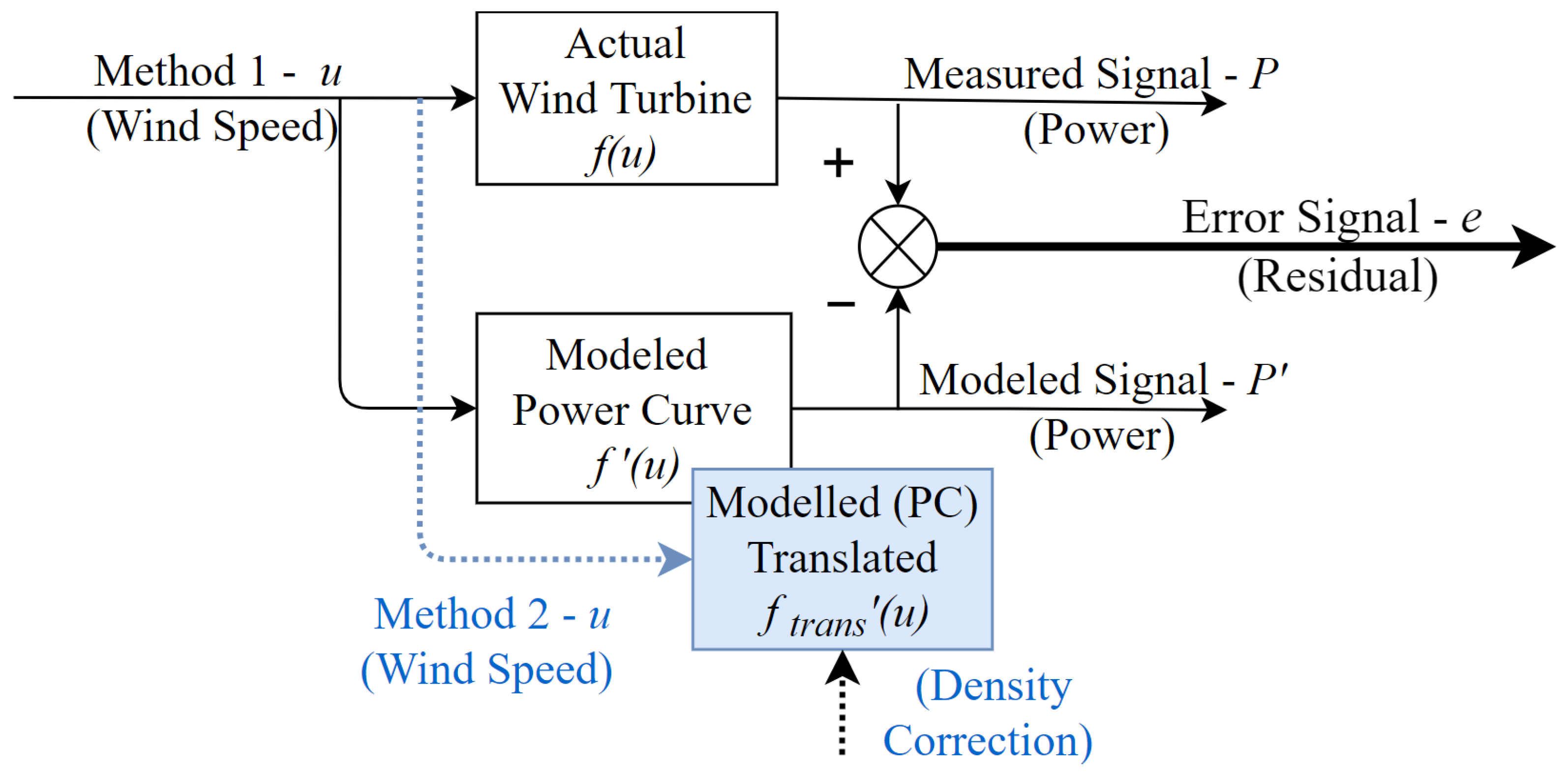
Figure 1 presents an overview of the residual generation process. The actual wind turbine is submitted to environmental influences (e.g., the wind speed), labeled u and consequently produces electrical power (the produced power shown as the actual/measured system output labeled P). If the same process is modeled, through any of the mathematical process modeling techniques represented by $f^{\prime }(u$), the output $P^{\prime }$ becomes the modeled system output. For Method 1, the power curve is modeled by the method of binning but regression, curve fitting, etc., can also be used. The difference between the measured and modeled outputs can be labeled as error $e$ or also commonly referred to as the residual. Figure 1 also shows Method 2 which uses the same environmental variable (e.g., wind speed) labeled u as input but data is corrected for density and translated to generate the corresponding modeled output $P^{\prime }$ through translated power curve relationship ${f_{trans}}^{\prime }\left(u\right)$.

2.3. Limitations and Need for Further Dispersion Reduction

The use of power curves for condition monitoring is, however, not without challenges. The data dispersion around the power curve adds to the difficulty of change detection. The appropriate handling of this dispersion and the variations caused by other operational and environmental conditions become key aspects when considering power curves as monitoring tools. The decreased data dispersion could result in increased detection performance.

One of the key objectives of this research is thus to evaluate the power-based fault detection methods on their ability to address such variability and data dispersion. An additional way to address data dispersion in the form of a multi-turbine approach is proposed and consequently, a potential improvement in detection performance is expected. An emulation of the impact of wind characteristics on the power curve and the evaluation of their impact on the detection performance of a fault detection method is also tested in the following sections.

3. Reducing Dispersion and Improving Detection: Multi-Turbine Approach

As briefly referred to earlier, the multi-turbine approach has been shown to successfully reduce the dispersion in temperature-based methods. Power-based methods also stand to benefit from the decrease in data dispersion and hence, an increase in detection performance. The rationale, assumptions and algorithm for a farm-level multi-turbine comparison using power curves are presented hereafter.

3.1. Rationale for the Multi-Turbine Approach and General Principle

To benefit from the farm level turbine comparison, certain assumptions need to be made. Although the empirical evidence of comparing the production of one wind turbine to the other is quite intuitive in the industrial context, certain methodological prerequisites are imperative for this comparison to build its objective foundations. For a “multi-turbine” comparison to be valid, the following assumptions need to hold:

• All wind turbines in one wind farm are supposed to be homogenous, i.e., of the same make and model, installed at the same time.

This generally holds true as the make and model of wind turbines are selected before installation and most wind farms are constructed in one go. This makes the wind farm operationally homogeneous.

• All wind turbines in one wind farm are subject to the same environmental variations (wind speed, wind direction, air density, ambient temperature, etc.)

This generally holds true as well, since all WTs on a wind farm are geographically concentrated and relatively affected by the same environmental variations since weather conditions are roughly the same over the entire wind farm. This makes a wind farm relatively homogeneous or at least environmentally consistent.

Once these assumptions hold true, the principle of ‘farm reference’ can be leveraged. The principle dictates that despite the highly stochastic nature of the wind, the overall behavior of all turbines within a wind farm evolves in tandem. Consequently, a global farm reference behavior in normal circumstances can be learnt. Any deviation of a wind turbine from this ‘farm reference’ (the normal evolutionary behavior of the overall farm), can be considered an anomaly and used for fault detection.

3.2. Implementation: Multi-Turbine Algorithm

Thus far, we have seen two power-based residual generation methods for single wind turbine fault detection (Methods 1 and 2 in Section 2.2.1 and Section 2.2.2). Provided the prerequisites identified in the previous section are met, a multi-turbine algorithm can be developed.

The principle of the multi-turbine approach is implemented as an extension to the above listed ‘mono-turbine’ fault detection residuals. The proposed ‘hybrid mono-multi-turbine’ approach resorts to a comparison of the single-turbine residuals, assuming that, under the fault-free situation, the evolution for all the turbine residuals within the same wind farm is the same. If one of the residuals departs from the others, then it is considered evidence of a fault on the corresponding turbine. This new strategy is a hybrid multi-level (turbine and farm level) approach to generate a monitoring indicator that will be used for fault detection and performance evolution for this research.

The algorithm for the multi-turbine indicator creation for temperature variables is presented in detail by the authors in [31]. The inspired and modified three-step hybrid mono-multi health indicator creation strategy for the power-based approach can be summarized as follows.

$R^i{}_{mono}\left(k\right)$ is the value of the residual $R_{mono}$ from turbine $i$ at time $k$. Let $N$ be the number of turbines in the wind farm. For each turbine $i$, with $i$ varying from 1 to $N$, the multi-turbine fault indicator $R^i{}_{multi}\left(k\right)$ is built at time $k$, as follows:

1.

The mono-turbine residual for each turbine $i$ in the farm is first calculated depending on the Method chosen (1 or 2), but globally as a difference of measured $P$ and modeled power $P^{\prime }$ given by Equation (1):

$$R_{mono}^i\left(k\right)=P^i\left(k\right)-{P^{\prime }}^i\left(k\right)$$

(1)

2.

The farm reference $R_{farm}\left(k\right)$ for turbines 1,… $N$ is calculated using the $R^i{}_{mono}\left(k\right)$ at the turbine level, using Equation (2) as follows:

$$R_{farm}\left(k\right)=media{n}_{\left(l=1,\dots N_L\right)}\left(R_{mono}^l\left(k\right)\right)$$

(2)

The farm reference is calculated using the median since the median is less sensitive to outliers and abnormal values than the mean. The farm reference will not be sensitive to the possible extreme values present in the residuals of the turbines used to calculate $R_{farm}\left(k\right)$. For the practical implementation, the farm reference is computed if more than half of the turbines used to calculate the farm reference operate in normal conditions and their data is available. $N_L$ is the minimum number of turbines required for the calculation of $R_{farm}$.

3.

The multi-turbine residual fault indicator $R^i{}_{multi}\left(k\right)$ is then calculated for each turbine $i$ as the difference between the mono Residual $R^i{}_{mono}$ and Reference $R_{farm}\left(k\right)$ using Equation (3).

$$R_{multi}^i\left(k\right)=R_{mono}^i\left(k\right)-R_{farm}\left(k\right)$$

(3)

This multi-turbine fault indicator $R^i{}_{multi}\left(k\right)$) is a result of the hybrid mono-multi-turbine residual generation and can now be used for the performance analysis of fault detection methods. This strategy will be referred to as hybrid mono-multi-turbine or for brevity, hybrid multi-approach from here onwards. The same process is repeated to calculate the multi-turbine residuals for all wind turbines in the wind farm. $R_{mono}^i\left(k\right)$residuals are assumed to carry information on the individual turbine deterioration and when used in the multi-turbine configuration as proposed, can provide useful insights into the state of the turbine. The overview of the proposed hybrid mono-multi-turbine approach is presented in Figure 2.

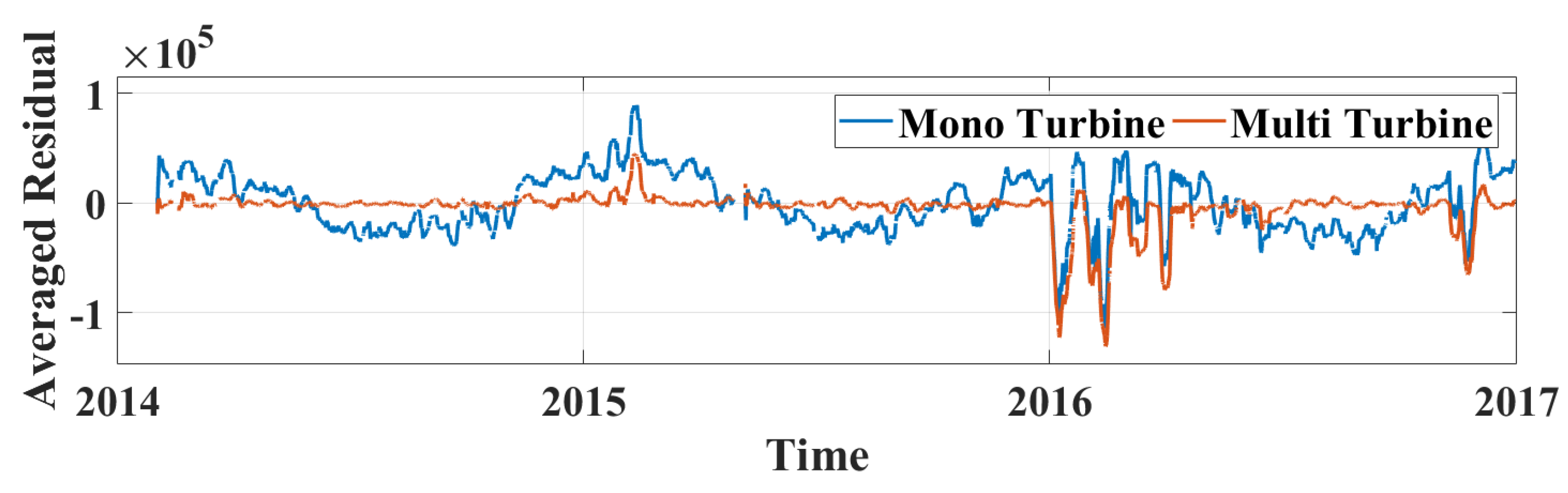
Figure 3 presents the examples of mono-turbine residual $R_{mono}$ calculated using Method 1, presented in Section 2.2.1, and the residual $R_{multi}$ calculated using the multi-turbine approach presented so far. The moving average of 1 week is calculated for both signals presented. The example presented shows fault-free data for the years 2014–2015 and a signal containing a fault induced in the year 2016. The fault used in the example is detailed in Section 4.3; Figure 7.

The objective of this research contribution then becomes to evaluate the “hybrid multi” turbine approach for power-based fault detection techniques in different settings. This is achieved using the rich capabilities of the realistic simulation framework developed by the authors in [37]. To achieve that, first, the expansion of a realistic simulation framework to incorporate multi-turbine configurations is required.

4. Numerical Experimentation and Discussion

The simulation framework proposed by [37] is used to generate realistically simulated data. It provides a means to generate close to real power produced values depending on the external environmental conditions such as the wind speed and the external temperature. The simulation framework has been extended to include the influence of the nature of wind (turbulent or laminar) on the power produced. It enables the evaluation of the detection performance of both fault detection methods (1 and 2) in their hybrid multi-turbine implementations. The simulated data generation framework accounting for the realistic environmental variability, i.e., the variation in the nature of wind (laminar vs turbulent) is discussed in the following sections.

4.1. Simulated Data Generation

The realistic simulation of produced power data for a single turbine is a two-step process. First, a reference power curve representing the normal behavior is required. Second, the data dispersion learnt on real data is added to this reference power curve as a function of site wind speed and temperature to generate simulated power data. The framework for mono-turbine data simulation is detailed in [37]. It realistically captures the data dispersion due to the varying wind speed and external temperature variation. This framework has been modified to include another source of variation in the environmental condition, i.e., the nature of the wind flow, switching between laminar and turbulent.

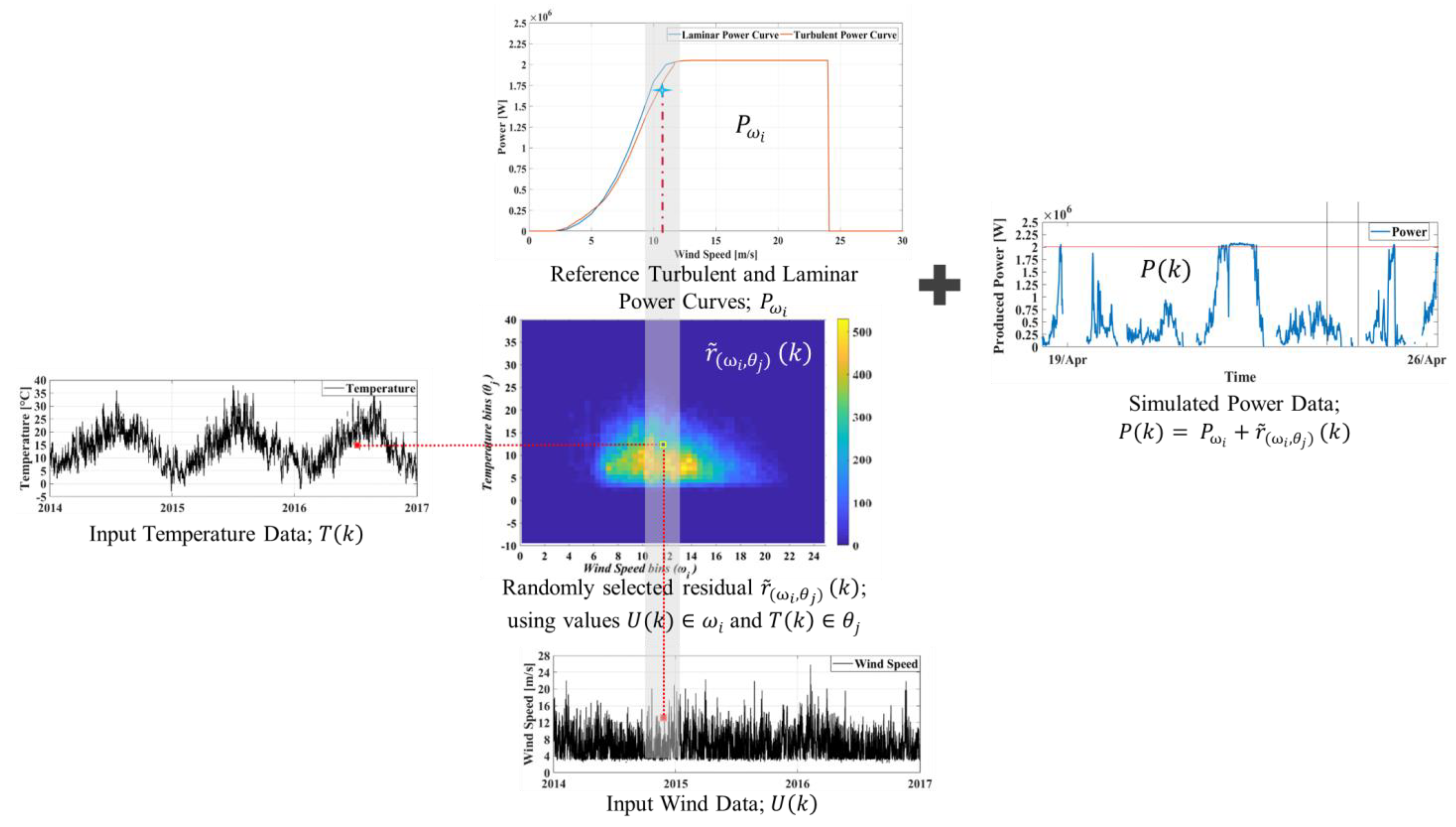
Figure 4 overviews the simulation process and the approach taken for incorporating the wind variability. To simulate a 10-min power time series, the simulation process is used with the wind speed and external temperature time series $\left(U\left(k\right),T\left(k\right)\right)$ measured on a wind turbine as inputs. $\left(U\left(k\right),T\left(k\right)\right)$ are times series of wind speeds and temperatures recorded every 10 min where $k$ is the time index.

At each time stamp $k$, the values of this “input” pair of environmental parameters (Wind $U\left(k\right)\in {\omega }_i$ and Temperature$T\left(k\right)\in {\theta }_j$) are used to select the corresponding reference power value and a dispersion value, extracted from a residual matrix populated with data from a different turbine. Thus, the simulated power produced is the sum of two terms as represented by Equation (4).

• The power is produced using a power curve reference.
• An additional residual mimicking the real dispersion observed around a real power curve. The additional residual is randomly selected out of several values previously extracted from a real power curve of a wind turbine when the machine operated during the same environmental conditions (wind speed and temperature range $({\mathsf{\omega }}_{\mathrm{i}},{\theta }_j)$.

  $$P\left(k\right)=P_{{\mathsf{\omega }}_i}+{\tilde{r}}_{\left({\mathsf{\omega }}_i, {\theta }_j\right)}\left(k\right)$$

  (4)

  where
  $P\left(k\right)$ is the simulated power output for the input ($U\left(k\right), T\left(k\right))$ pair;
  $P_{{\omega }_i}$ is the reference power curve;
  ${\tilde{r}}_{\left({\mathsf{\omega }}_i, {\theta }_j\right)}\left(k\right)$is the dispersion residual selected randomly from $\left(l\right)$ entries in the reference bin (${\mathsf{\omega }}_i$,${\theta }_j$) with $\begin{array}{c}U\left(k\right)\in {\omega }_i\\ T\left(k\right)\in {\theta }_j\end{array}\}$.

Simulation of the Variable Nature of Wind

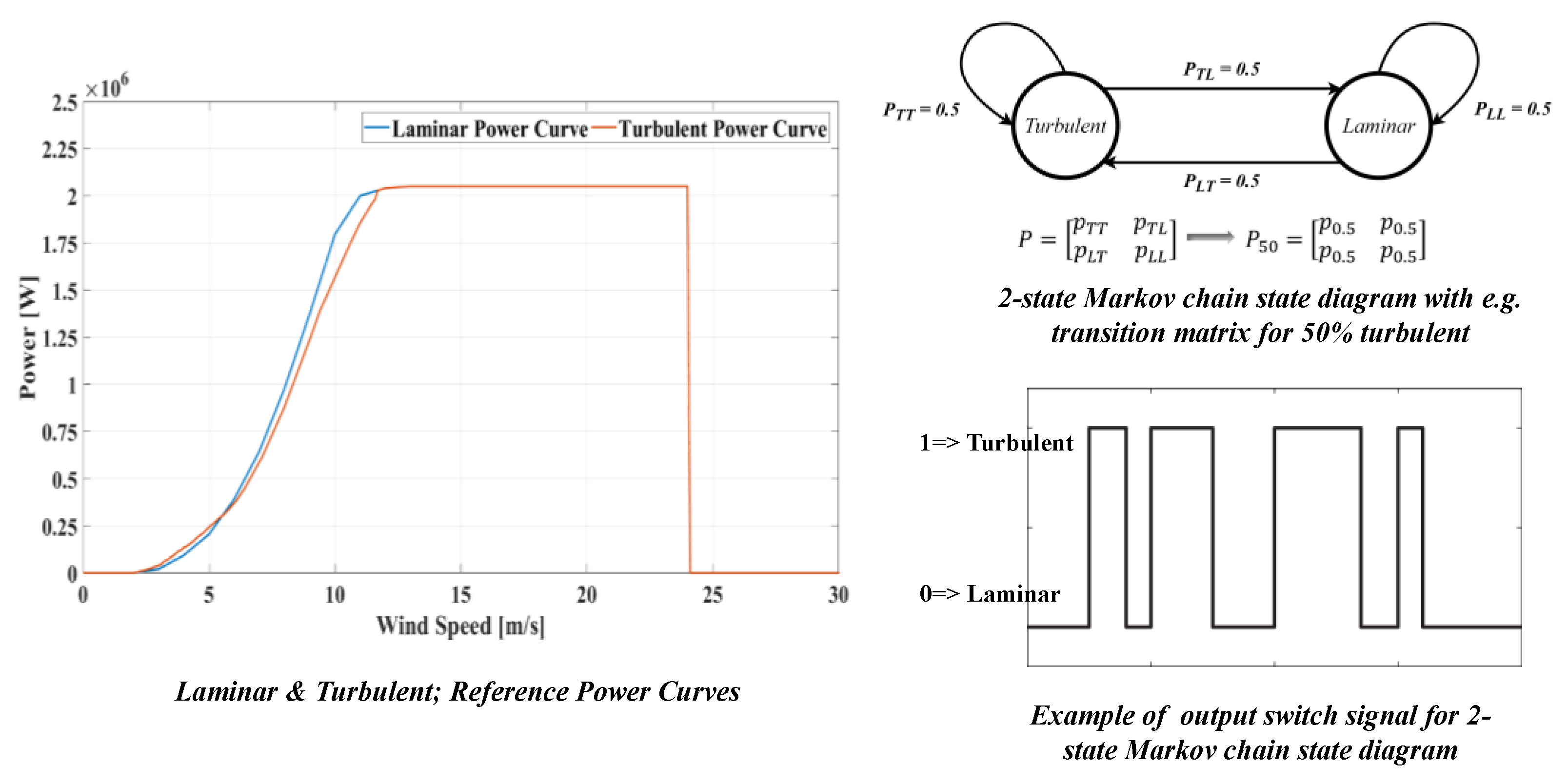
There are several ways to capture the difference between a laminar or turbulent wind flow. For this implementation, this variation is modeled by using different power curves. When the wind is laminar, a laminar power curve is used, $P_{{\omega }_i}=f_{laminar}\left({\omega }_i\right)$, and when the wind is turbulent, a turbulent power curve is used, $P_{{\omega }_i}=f_{turbulent}\left({\omega }_i\right)$. The literature presents various cases where increased turbulence decreases the produced power for higher wind speeds and increases the reference power slightly for lower wind speed durations [38,39]. Since the increased turbulence impacts the power curve negatively, this provides the inspiration for modeling two reference power curves. Then, to capture the stochastic nature of wind, which constantly and randomly switches between turbulent and laminar, a two-state Markov chain model is proposed [40]. The changing nature of wind from laminar to turbulent is emulated, depending on the probabilities set in the transition matrix. The relevant transition matrix for the required state (turbulent/laminar) determines the percentage of time the relevant reference power curve (laminar/turbulent) is chosen.

The simulated profile is created using the measures at a given time $k$ of wind speed $U\left(k\right)$ and the external temperature $T\left(k\right)$ recorded on a real wind farm. The corresponding reference power, $P_{{\omega }_i}$ is computed from the turbulent or laminar power curves, depending on the wind state at time $k$, selected from the output switch signal created with the two-state Markov chain. A residual is then randomly selected from the data dispersion matrix, using the bin corresponding to the wind speed $U\left(k\right), T\left(k\right)$ and added to the power produced (Equation (4)).

Figure 5 shows the laminar and turbulent power curves. Additionally, in the Markov chain state diagram, the transition matrix for the 50% turbulent $P_{50}$ wind scenario and an example of the output switch signal are also presented.

Using this approach, the power data is then simulated using these laminar and turbulent power curves.

The power produced is computed for each turbine of a wind park. To model the “park effect”, the environmental profile $\left(U\left(k\right), T\left(k\right)\right)$ used to generate the data is the same for all the turbines of the park. The “turbulent” or “laminar” state is the same for all the turbines in the park and the switch between turbulent and laminar mode is done at the same time for all the turbines under normal conditions. To model the variability between turbines, the residual added to the power produced is randomly selected from different dispersion matrices, one per each turbine of the park.

4.2. Simulation Protocol

For the simulation framework, data from five different wind farms (27 wind turbines) is chosen. These wind farms represent data from a variety of environmental and operational sources. The simulation output is organized in the form of a simulation matrix (

Table 1. Simulation Matrix (SM).

			Operational Profiles
			Farm-V						Farm-L				Farm-D						Farm-S						Farm-C
Environmental Profiles			V1	V2	V3	V4	V5	V6	L1	L2	L3	L4	D1	D2	D3	D4	D5	D6	S1	S2	S3	S4	S5	S6	C1	C2	C3	C4	C5
	Farm-V	V1
	Farm-L	L1
	Farm-D	D1
	Farm-S	S1
	Farm-C	C1

). Each case represents a simulated power profile. The environmental profile $\left(U\left(k\right), T\left(k\right)\right)$ is expressed in rows while the turbine used to populate the residual matrix is in columns. For instance, the case (Farm-V: V1, Farm-L: L2) contains the power simulated from the environmental profile of the first wind turbine of Farm-V, and the residuals collected from the second wind turbine of Farm L.

As detailed in the multi-turbine residual generation algorithm, the simulation and eventual performance analysis for this research requires a multi-turbine residual calculation $R_{multi}$. This multi-turbine residual requires at first, the calculation of a mono-turbine residual $R_{mono}$ calculated for each of the turbines and thus, the generation of power profiles for all turbines within a park.

For each cell of the simulation matrix in the multi-turbine implementation corresponding to the turbine $T_{ij}$ of the wind farm $P_j$, all turbines of the farm $P_j$ are simulated with the same environmental (wind, temperature) profile. The fault is introduced in the turbine $T_{ij}$ and the multi-turbine residual $R_{multi}$ for turbine $i$ belonging to park $P_j$ is calculated using all mono-turbine residuals for the turbines on farm $P_j$. The process is repeated for each turbine on the farm, one by one.

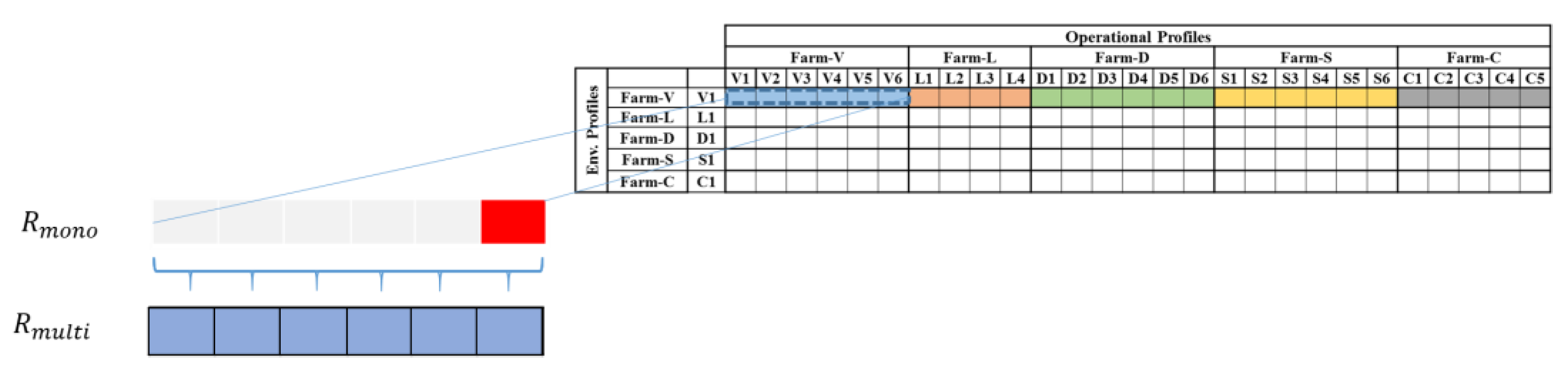
Figure 6 presents the simulation matrix (SM). Each color represents a different wind farm. The multi-turbine residual $R_{multi}^i$ can be calculated using the data streams/mono-turbine residuals from the uniquely color-coded portions of the simulation matrix for all rows. This is consistent with the farm labels of V, S, D, S and C for the operational profiles (data dispersion sources). The rows in Table 1 and Figure 6 signify that only the environmental profile of the first turbine, i.e., V1, S1, D1, S1 and C1 is taken as representative of the whole wind farm.

We note here that for the sake of this work, we consider all turbines $T_{ij}$ of the wind farm $P_j$ to have the same environmental (wind, temperature) profiles. This comes from the fact that a wind farm concentrated in a limited geographical location experience the same environment. However, although globally consistent, there are slight offsets or variations in the environmental measurements of each wind turbine in a wind farm. To restrict the scope of this work, we limit our analysis to the row-based implementation for multi-turbine scenarios as it is sufficiently representative. This means that we consider identical environmental profiles for all turbines in a wind farm and ignore the minor intra-turbine variations.

Once the simulation matrix is populated with multi-turbine performance indicators, comprehensive performance analysis can be performed.

4.3. Performance Evaluation

Within the overall proposed framework, once the realistically simulated data time series are generated and implementation residuals calculated, performance evaluation metrics are required. Any analysis is incomplete without a rigorous performance evaluation criterion. As one of the key objectives of this research is to evaluate any detection performance gain achieved by using the multi-turbine approach, an evaluation mechanism becomes critical.

The detection of an occurring fault is usually made by deciding on a baseline for what is normal or acceptable and then setting a threshold on the normal behavior. The creation of a detection threshold is a delicate and difficult task since the fault indicators are not perfect and vary even when there is no fault. A compromise must, therefore, be made between the detection of real defects and the number of false alarms that the system may generate.

The performance indicator used in this work is the probability of detection (PD) for a given value of the probability of false alarms (PFA). This relationship, in classical signal theory, is called the receiver operating characteristic or ROC curve. In this research, the detection threshold is set, so that PFA is equal to 10%. The performance indicator for this evaluation is its corresponding PD. $P{D}_{10}$ provides a useful indicator as it represents a relatively descriptive and acceptable tool for analysis.

The simulated data and consequently the multi-turbine residual generated using this data is divided into three sections, each lasting one year. Year 1 and Year 2 are normal condition periods. Year 1 is used to learn the power curve model; Year 2 is used to set the detection threshold value Th. Year 3 is the ‘fault’ period and the detection performance indicator is calculated on it. Hence, $P{D}_{10}$ is the probability of detection for a 10% false alarm rate calculated for $R_{multi}^i$ using Equation (5).

$$P{D}_{10}=\frac{No. of samples below threshold \left(Th\right)}{Total No. of data samples in the fault period}$$

(5)

where $Th$ is set such as $PF{A}_{10}$ = 0.1 (10% PFA)

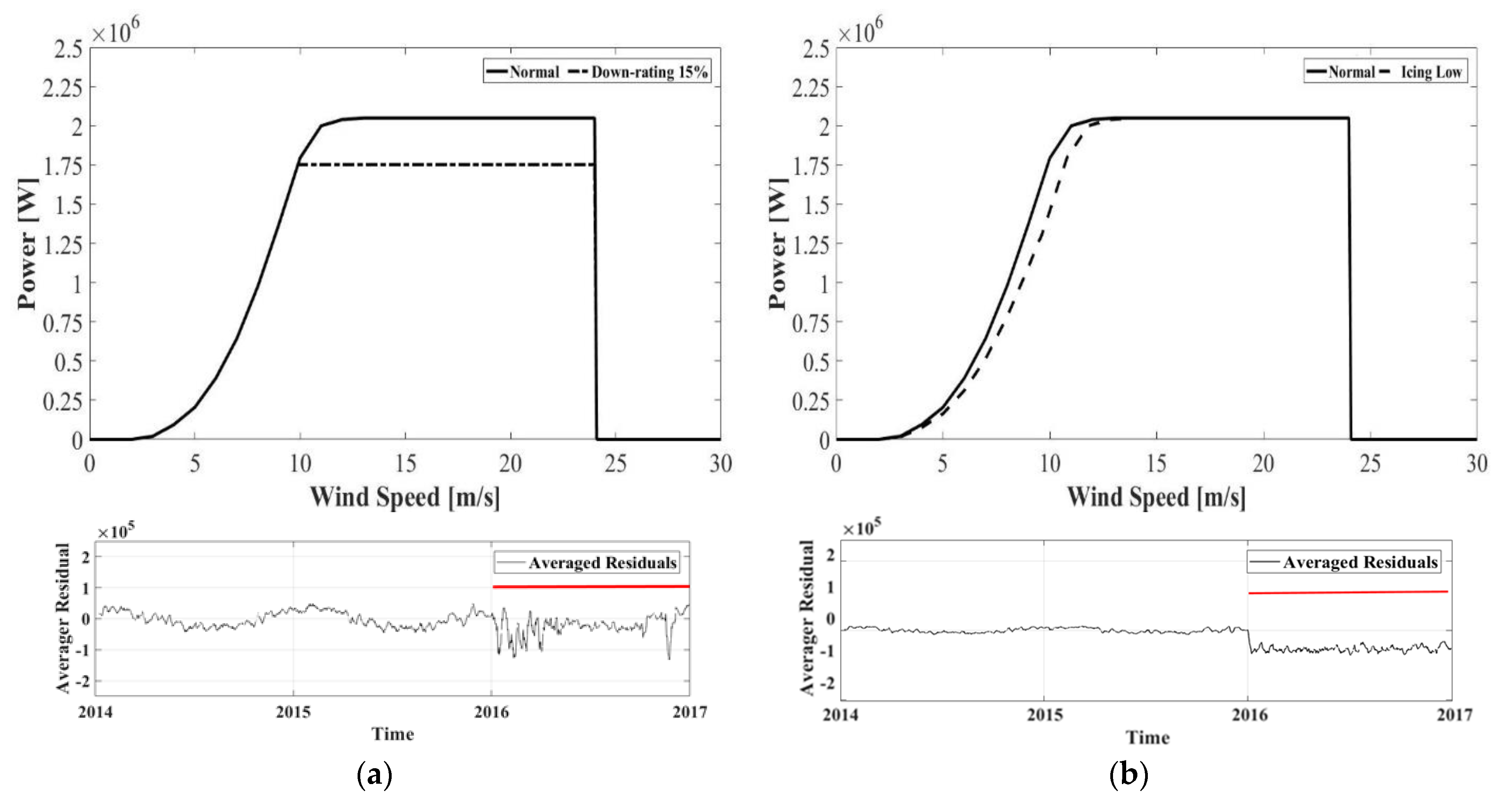
Different intensity levels of fault signatures are generated and considered for analysis. The reference power curves and corresponding residuals generated using Method 1 for two fault scenarios simulated and evaluated are presented in Figure 7 and described below.

• Down-Rating 15%: As shown in Figure 7a, this fault type is characterized as a downward shift for only the higher wind speeds of the power curve. This impact also appears as a downward shift in corresponding residual only when the wind speed is higher. The downward shift is not uniform for all values of the operational power curve but is only visible intermittently as visible in the corresponding residual.
• Icing 5%: As shown in Figure 7b, this fault type is characterized as a shift in the operational part of the power curve [41]. This impact also appears as a downward shift in the corresponding residual. The downward shift uniformly appears for all values of the operational power curve (between cut-in and nominal wind speeds).

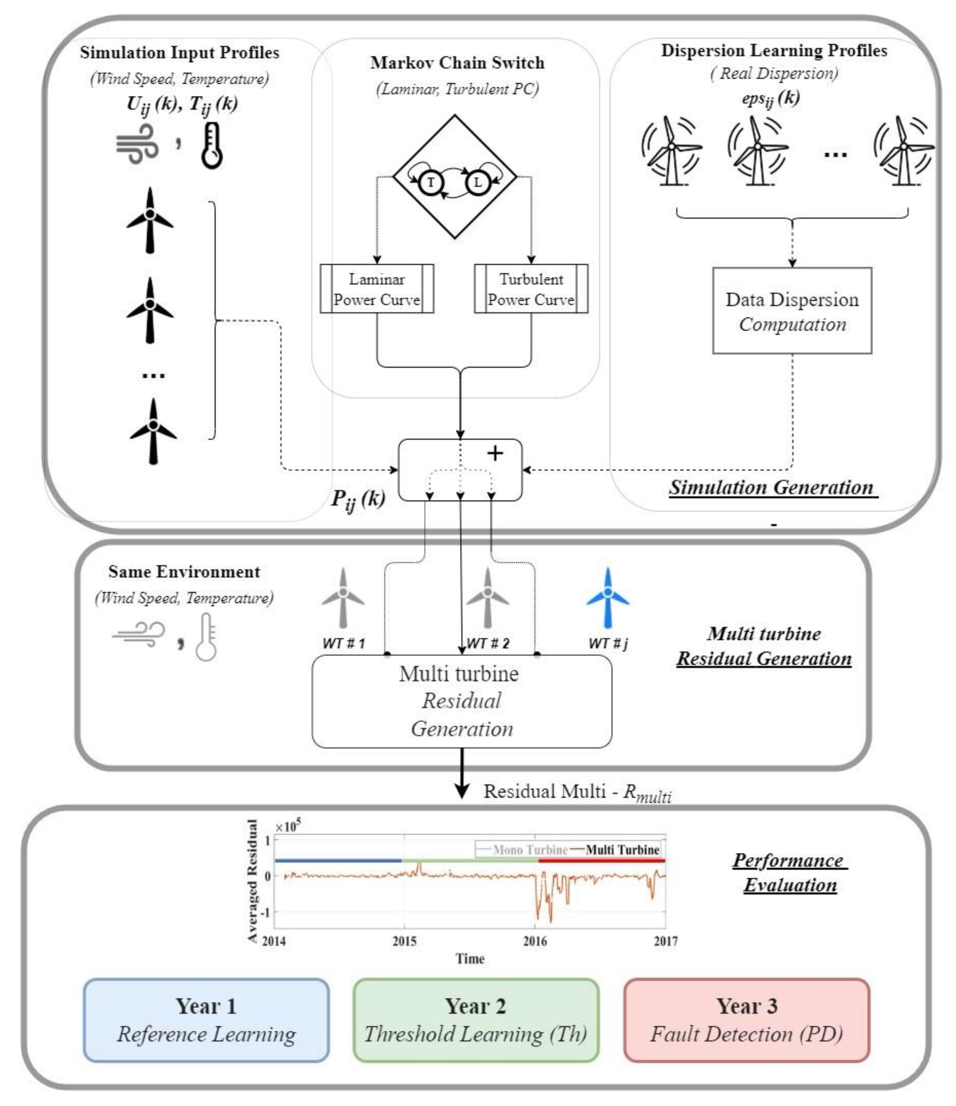
The overall multi-turbine simulation framework and the experimental setup detailed so far are presented in Figure 8.

4.4. Results and Discussion

The impact of using a multi-turbine approach versus a mono-turbine approach on the detection performances of fault detection methods is evaluated on two specific faults, (Down-Rating 15% and Icing 5%), each impacting the wind turbine production in a different way. Method 1 and Method 2, presented in Section 2, are used for the analysis. Method 1 is the baseline residual generation method, while Method 2 aims to decrease the data dispersion around the power curve by air density correction. The results for both scenarios for two faults (Down-Rating 15% and Icing 5%) are presented hereafter. In the first part, the results obtained by Method 1 in its mono- and multi-turbine versions are presented in a visual way. Then, the performances obtained by Method 1 and Method 2 in their mono- and multi-turbine versions are compared. Finally, the impact of turbulence on the performances of Method 2 is analyzed.

4.4.1. Performance Comparison of Mono- and Multi-Turbine Approaches—No Turbulence

As referred to earlier, Method 1 is used as the turbine level residual generator in step 1 for the fleet level multi-turbine implementation. To have a representative quantification of global performance, two fault types, Down-Rating 15% and Icing 5% are considered. Both visual and statistical results are presented and discussed in the following sections.

Note here that for brevity, the proposed hybrid mono-multi-turbine approach will be referred to as a ‘hybrid multi’ configuration hereon.

Visualization of the Results Using the Simulation Matrix

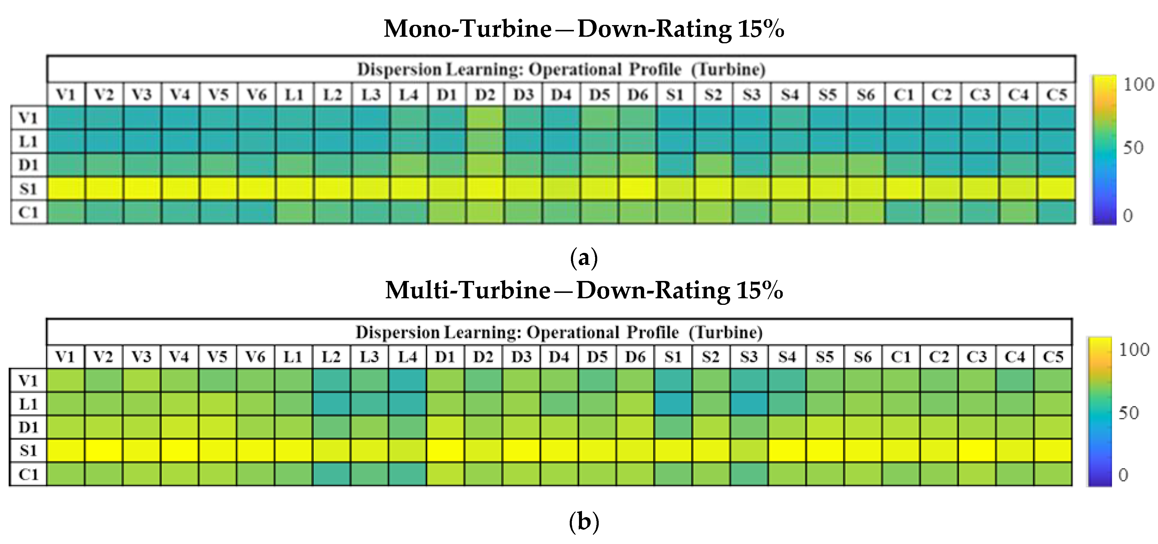
The performances obtained with Method 1 are first analyzed with the fault Down-Rating 15%. Each case of the simulation matrix is populated with its corresponding performance indicator $P{D}_{10}$., the simulation matrix thus becomes the performance evaluation matrix (PEM). Figure 9 shows the PEM calculated for the Down-Rating 15% fault case using Method 1 in ‘mono-turbine’ implementation. The three-level color scale goes from blue, green to yellow (0–100) for absolute values of performance indicators. It can be seen from the shades, that globally, the detection performance of Method 1 is low for all the farms tested, except for Farm S. This exception has to do with the specific fault signature and the wind distribution for Farm S. The wind distribution for Farm S shows a higher proportion of wind speeds between 8 and 16 ms⁻¹ (when compared to the other farms), which activates more the fault signature of the default “Down-Rating 15%”. See Figure 7a and Figure 10 and reference [15] for further details.

Figure 9b shows the $PEM$ matrix calculated for the Down-Rating 15% fault case using Method 1 in the ‘hybrid multi’ implementation. The color scale for this result is consistent with that used earlier (Blue-Green-Yellow). At a first glance, it is clearly visible from the much lighter shades as compared to Figure 9a that globally, the detection performance of Method 1 in the ‘hybrid multi’ configuration is significantly higher for all the farms tested. This gain is quantified at around 16 percentage points (pp.) for Down-Rating 15% and will be reported later along with the mean detection values for both approaches and their 95% confidence intervals.

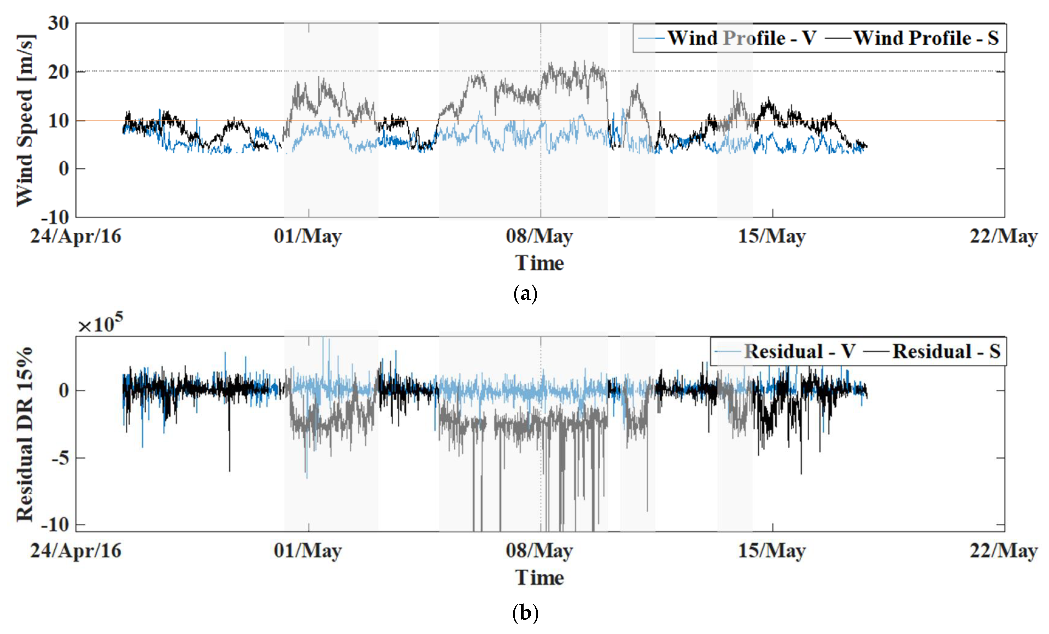
Figure 10 further elaborates the unique behavior of Farm S compared to other wind farms. Farm S is located at a site with onsite wind distribution shifted towards higher wind speeds. For the fault type Down-Rating 15%, this results in frequent excitation of the fault signature as compared to other wind farms and hence, a more visible fault signature, resulting in higher detection values of $P{D}_{10}$ for Farm S. Figure 10a shows the wind profile for two wind farms, S and V, while Figure 10b presents the corresponding mono-turbine residuals of both wind farms, in the case of Down-Rating 15%.

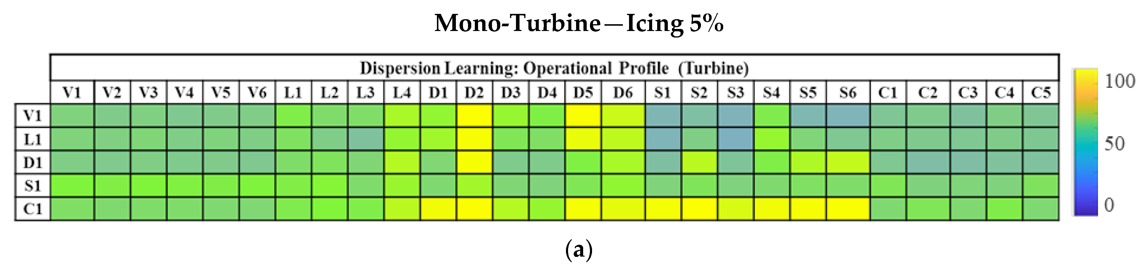
Fault Type Icing 5%

Similarly, for better visual representation, the PEM for fault type Icing in both scenarios (mono and hybrid multi) is useful. The $P{D}_{10}$ indicators calculated for the Icing 5% fault case using Method 1 in ‘mono-turbine’ implementation are shown in Figure 11a. The three-level color scale goes from blue to green to yellow for absolute values (0–100) and is consistent with the previous implementation. It can be seen from the bluish-green shades that globally, the detection performance of Method 1 is low for all farms tested with a few exceptions.

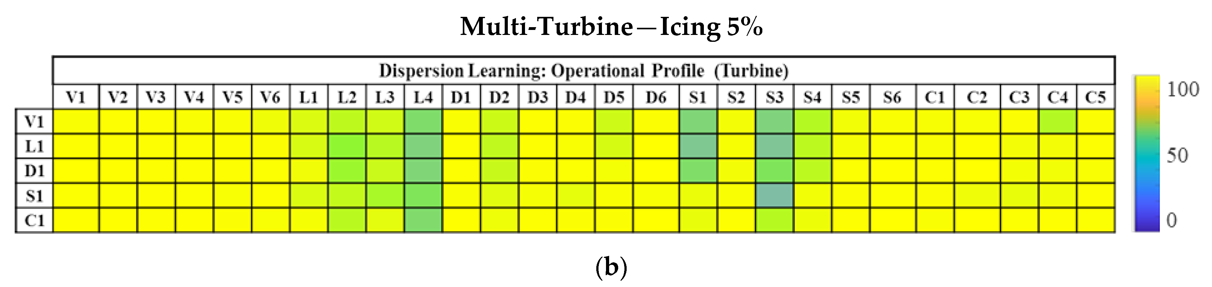
Figure 11b shows the $P{D}_{10}$ indicators calculated for the Icing 5% fault case using Method 1 in the ‘hybrid multi’ implementation. The over-whelming shade of yellow is clearly visible in Figure 11b. Even at a first glance, it is clearly visible that globally, the detection performance of Method 1 for ‘hybrid multi’ implementation is significantly higher for Icing 5% and for all farms tested. As visible, the detection performance gain of this fault family is higher than the gain observed for the Down-Rating. A 45 percentage point (pp.) increase in detection performance is reported when using the ‘hybrid multi’ approach as compared to the simple mono-turbine strategy for the fault type Icing 5%. These quantified results are reported in the following sections.

4.4.2. Performance Comparison between Method 1 and Method 2

The visual representation of PEM for the fault type Down-Rating 15% with Method 1 has been presented so far. Intuitively and visually, the performance gain for using the ‘hybrid multi’ turbine approach when residuals are produced with Method 1 is clear. The same results can be quantified by computing the mean of the PEM matrix and by calculating the 95% confidence interval for these values. This will help evaluate the quantifiable gain in terms of the mean performance indicator ($P{D}_{10}$).

Table 2. (a). Performance comparison of Method 1 vs Method 2—Mono-Turbine config. (b). Performance comparison of Method 1 vs Method 2—Multi-Turbine config. (c). Performance gain of Multi-Turbine over Mono-Turbine.

	(a)
	Mono-Turbine
	Down-Rating 15%			Icing 5%
	Method 1	Method 2	Gain (pp.)	Method 1	Method 2	Gain (pp.)
Performance Indicator (PD10)	43.22 ± 1.4 pp.	56.72 ± 2.20 pp.	13.5 pp.	42.95 ± 4.08 pp.	63.34 ± 4.42 pp.	20.4 pp.
	(b)
	Multi-Turbine
	Down-Rating 15%			Icing 5%
	Method 1	Method 2	Gain (pp.)	Method 1	Method 2	Gain (pp.)
Performance Indicator (PD10)	57.62 ± 3.20 pp.	57.67 ± 3.33 pp.	~0.05 pp.	88.05 ± 3.45 pp.	90.53 ± 2.73 pp.	~2 pp.
	(c)
	Mono-Turbine vs. Multi-Turbine
	Down-Rating 15%			Icing 5%
	Method 1	Method 2		Method 1	Method 2
Performance Gain (pp.)	14.4 pp.	~1 pp.		45 pp.	27.2 pp.

reports the mean detection performance indicator values (in percentage point, pp.) and its 95% confidence interval for ‘mono’ and ‘hybrid multi’ approaches and the results are reported for the fault types Down-Rating 15% and Icing 5%.

Table 2a shows the performances obtained by Method 1 and Method 2 in the mono-turbine approach for Down-Rating 15% and for Icing 5%. As expected, Method 2 performs better than Method 1 for both fault cases. For Down-Rating 15%, a clear gain of ~13.5 pp., and for Icing 5%, a gain of 20.4 pp. in detection performance is observed.

Table 2b shows the performances obtained by Method 1 and Method 2 in the multi-turbine approach for Down-Rating 15% and for Icing 5%, and Table 2c summarizes the gain obtained when switching from a mono-turbine approach to a multi-turbine approach for Method 1 and Method 2 and for the two fault cases.

Method 1 clearly benefits from the multi-turbine approach. The detection performance increases from 43.22 pp. to 57.62 pp. for Down-Rating 15% and from 42.95 pp. to 88.05 pp. for Icing 5%. For Method 2, the detection performance increases from 63.34 pp. to 90.53 pp. for Icing 5%. However, no increase in performance is observed for Down-Rating 15%. This can be explained by the fact that optimal detection performances were already reached with the mono-turbine approach with Method 2. Indeed, the fault signature of Down-Rating 15% is a loss of production during periods of time when the wind speed is higher than 10 m/s. The wind speed distribution of the five French wind farms used for the simulation shows that this situation does not happen so often. Though in the simulation, the default is present during the whole year, its effect, i.e., the loss of production, is not visible during the whole year. The consequence of it is the setting of a maximum attainable limit to $P{D}_{10}$, which measures the percentage of time the fault is detected during the whole year. The situation is different for Icing 5%, whose signature is a decrease in performance when the wind speed is below 13 m/s and is observable most of the year (in the simulation, icing can occur even if the temperature is not below 0 °C). Thus, one can conclude that both methods benefit from the multi-turbine approach with a gain of performance ranging from 14.4 pp. to 45 pp.

Moreover, one can see that when the multi-turbine approach is used, the performance of Method 1 becomes comparable to Method 2, for the two fault cases. The main difference between Method 1 and Method 2 is that Method 2 aims to reduce the dispersion around the power curve by using the external temperature values to calculate the residuals. Method 1 uses the power curve in a rather simple way, as it requires only the value of the wind speed to build the residuals. This means that a rather simple method, which requires measuring only the wind speed, can perform as well as a more advanced method which requires measuring both the wind speed and the temperature because the multi-turbine approach significantly reduces the impact of data dispersion on the residuals.

4.4.3. Multi-Turbine Performance Evaluation under Turbulence (50%)

As briefly explained earlier, turbulence intensity adds to the difficulty of detection. It decreases the performance of the turbine and increases the data dispersion around the power curve. It is interesting to quantify the impact of turbulence on detection performance. The results obtained when the wind is turbulent for 50% of the time are now presented.

The extended hybrid multi-turbine simulation framework is set up to evaluate the detection performance of the second fault detection method (Method 2). The interest for this configuration is to evaluate the detection performance in a hybrid multi-turbine configuration and to subject Method 2 to turbulent wind conditions. This additional variation is introduced, as explained in the earlier sections.

Table 3. Impact of turbulence on detection performance of Method 2—Mono and Multi-Turbine.

	Method 2
	Down-Rating 15%			Icing 5%
	Mono-Turbine	Multi-Turbine		Mono-Turbine	Multi-Turbine
No Turbulence	56.72 ± 2.20 pp.	57.67 ± 3.33 pp.		63.34 ± 4.42 pp.	90.53 ± 2.73 pp.
			Multi-turbine Detection Gain (50% Turb.)			Multi-turbine Detection Gain (50% Turb.)
Turbulence 50%	44.18 ± 3.80 pp.	54.72 ± 3.43 pp.	10.54 pp.	53.70 ± 3.38 pp.	90.14 ± 2.66 pp.	28.61 pp.
Detection Loss Turbulence	12.54	2.95		9.64	0.39

reports the mean detection performance indicator for the mono and hybrid multi-turbine approach for the cases of no turbulence and 50% of turbulence. The increased variability introduced by the turbulent behavior is simulated, mono- and hybrid-multi-residuals are generated, and performance indicators are calculated and averaged. The results in Table 3 are reported for fault types, Down-Rating 15% and Icing 5%.

First, let us notice that turbulence has an important impact on the detection performance of Method 2. In the mono-turbine approach, $P{D}_{10}$ significantly decreases by 12.54 pp. for Down-Rating 15%, and by 9.64 for Icing 5% when 50% turbulence is added, compared to no turbulence. Now, when the multi-turbine approach is used, the impact of turbulence on the performance is strongly reduced. The loss is only 2.95 pp. for Down-Rating 15%. The detection performance is equivalent to that with no turbulence for Icing 5%. This means that the multi-turbine approach can reduce the dispersion induced by turbulence. The gain of using a multi-turbine approach is clearly visible in Table 3. With 50% of turbulence, the multi-turbine detection performance is 10 pp. higher than the mono-turbine approach for Down-rating 15% and 28.6 pp. higher for Icing 5%. The conclusion is, that turbulence negatively affects the detection performance of Method 2 but that the multi-turbine approach handles this impact better.

4.4.4. Summary of the Results

To summarize, we recall the following conclusions drawn from the analysis.

Normal conditions:

• The detection performance of Method 1 can be increased using the proposed multi-turbine approach. A mono vs multi gain of ~14.4 pp. for Down-Rating 15% and a gain of ~45.5 pp. for fault type Icing 5% has been reported for normal environmental conditions (Table 2).
• Method 2 gains from the multi-turbine approach as well. An average mono vs multi gain is ~27.2 pp. for icing (5%) under normal environmental conditions (Table 2).
• Method 1 and Method 2 reach equivalent performances when the multi-turbine approach is used.

Turbulent conditions:

• Method 2 in multi-turbine is better than mono-turbine implementation under a 50% turbulence scenario. This gain of Method 2 mono vs Method 2 multi is significant (10.54 pp. in Down-Rating and 28.61 pp. in Icing, respectively) (Table 3).
• Method 2 in multi-turbine configuration is relatively less sensitive to turbulence. For example, the detection loss for 50% turbulence is reported to be ~12.54 pp. for mono-turbine but ~2.95 pp. under the multi-turbine implementation of Method 2 for 15% Down-Rating. The same is true for Icing 5% where mono-turbine loses 9.64 pp. of its detection performance to turbulence vs. 0.39 pp. lost by the multi-turbine implementation of Method 2 (Table 3).

In conclusion, by comparing the performance of Method 1 and Method 2 in their mono- and multi-turbine implementation, it can be observed that both methods benefit from the multi-turbine implementation. In its multi-turbine implementation, in normal conditions, the performances of Method 1 become equivalent to that of Method 2. The hybrid multi-turbine implementation allows for reducing the variability due to environmental conditions (temperature, wind type). Hence, when implemented following a multi-turbine approach, a simple method such as Method 1 gains significantly in performance.

By comparing the performance of Method 2 in its mono- and multi-turbine implementation, it can be observed in both considered fault cases that (i) the presence of turbulence leads to a loss in fault detection performance—and (ii) in the presence of turbulence, the multi-turbine implementation improves the detection performance when compared to the mono-turbine implementation.

These conclusions, based on only two fault cases, cannot be considered general, and the observations still need to be thoroughly explained; to reach more general conclusions, further examination is required to gain a better understanding of the underlying mechanisms for a fault to happen and its signature on the power curve in the presence of turbulence to optimize the detection performance.

5. Conclusions and Perspectives

Three distinct contributions are made in this research. First, a hybrid multi-turbine implementation of fault detection methods based on a power curve has been proposed. Second, its implementation was made possible by extending and adapting a realistic simulation framework to include a hybrid single-multi-turbine configuration. Finally, a numerical and experimental performance analysis of the proposed hybrid multi-turbine implementation was presented.

In addition, to account for more realistic environmental variations, changes in the nature of the wind (from laminar to turbulent) were also included in the analysis. Two familiar fault detection approaches, Method 1 and Method 2, were tested in a multi-turbine approach. It was shown that the hybrid mono-multi-turbine detection strategy can significantly improve the overall fault detection capability of power-based methods, even under turbulent wind conditions.

It was also established that the hybrid multi-turbine approach performed better than the mono-turbine method, whatever the situation (normal or turbulent). The gain in detection performance for Method 1 using the multi-turbine approach is significant, while Method 2 also benefits from improved performance.

These results are consistent with the results obtained by the mono-multi hybrid solution, implemented for temperature-based defect detection methods [31]. Both contributions have profound implications in the industrial context, as any improvement in detection performance is highly desirable. Future work may include additional fault detection methods, other fault scenarios and turbulence intensity cases as well.