An Impedance Matching Solution to Increase the Harvested Power and Efficiency of Nonlinear Piezoelectric Energy Harvesters ^†

Abstract

Circuit theory and nonlinear dynamics are instrumental to design efficient energy harvesters for ambient mechanical vibrations. In this work, we show that an impedance matching networks can be designed that maximizes the harvested power, and improves the power efficiency. The proposed matching network achieves impedance matching at a single frequency, that can be chosen at will by the designer, and does not need to coincide with the resonant frequency of the harvester. Moreover, the matching network also increases the harvested power over a wide frequency bandwidth. According to our numerical simulations, the matching network increases the maximum harvested power by a factor greater than 3, and the power harvested over the whole frequency spectrum by a factor of 6. The frequency bandwidth can be further extended considering nonlinear energy harvesters. Even using the matching network designed for the linear case, performance is significantly nonetheless improved for the nonlinear harvester.

1. Introduction

Powering networks of miniaturized, wireless-connected electronic and electro-mechanical systems, sensors and actuators, namely the hardware substrate of the Internet of Things paradigm, is a major challenge. Classical solutions, such as disposable batteries, are not viable, because of their limited power density, lifespan, and the environmental hazards related to their disposal.

A fascinating solution consists of designing systems able to scavenge energy from the surrounding environment, where and when necessary, being the ultimate power source electromagnetic radiation, solar light, temperature gradients, or mechanical vibrations [1,2,3,4,5]. In particular, kinetic energy, in the form of mechanical vibrations, regular or random displacements and driving forces, is particularly attractive, because of its comparatively large power density and its widespread availability [6,7,8,9].

Irrespective of the working principle, energy harvesting systems are limited by the relatively small power density of the source, and by geometric constraints. For example, a linear harvester must be carefully designed in such a way that the oscillator’s resonance frequency matches the spectral range of environmental vibrations where most of the energy is concentrated. Unfortunately, the general rule is that the smaller is the size of an object, the larger its resonance frequency will be. Therefore, the realization of energy harvesters that are both miniaturized, and that work efficiently at the typical frequencies of ambient mechanical vibrations is problematic. Ingenious mechanical workarounds, including systems with a moving inertial mass capable of adapting their proper frequency to that of the external forcing, have been recently proposed [10,11]. As an alternative, nonlinear oscillators are widely believed to perform better than linear ones [12,13,14,15,16,17]. When compared to their linear counterparts, nonlinear energy harvesters show a wider steady-state frequency bandwidth and may exhibit multi-stability and even chaotic dynamics, thus suggesting that they can be more efficient especially in random and non-stationary vibratory environments [18,19,20,21].

Another limiting key factor is the impedance mismatch between the mechanical and electrical domains of the harvester, and the load, often represented by an electrical or electronic circuit. Several authors suggested that impedance matching can solve this problem [22,23,24,25,26,27]. To keep the analysis simple, these works either focus on linear systems [23,24], or fix the load resistance at the exact value to obtain maximum power transfer, and impose a resonance condition between the mechanical and electrical domains [22,25,26,27]. This simplifying hypothesis allows obtaining impedance matching with a simple shunt reactance in parallel with the load.

In practical applications however, the load resistance is a fixed parameter that cannot be chosen at will, and the power of mechanical vibrations could be concentrated in a frequency range well apart from the resonant peak of the harvester. This contribution extends our previous works [22,27], with particular reference to the aforementioned limitations. We show that interposing a matching network between the energy harvester and the resistive load, the harvested power and the efficiency are significantly increased. The matching network is a two port reactive network, designed to achieve impedance matching at a specific frequency that can be chosen at will by the designer, and that does not necessarily need to coincide with the resonant frequency of the harvester. Moreover, impedance matching can be obtained for any a priori fixed value of the load resistance. The matching network also increases the harvested power over a wide frequency bandwidth. According to our findings, the maximum harvested power is increased by a factor larger than 3, and the total harvested power over the whole frequency spectrum by a factor of 6. The matching network offers a relatively high, 50% efficiency at the frequency where the maximum power is absorbed, whereas the efficiency of the energy harvester with a purely resistive load decreases as the frequency is increased. Although there is little theory concerning the design of nonlinear systems, we show that the matching network designed for the linear harvester can be applied with benefit also to a strongly nonlinear energy harvester.

The paper is structured as follows: in Section 2, we derive the governing equations for the mechanical part of the harvester and the piezoelectric transducer. Using mechanical to electrical analogies, we develop an equivalent circuit model for the harvester. In Section 3, we apply circuit theory to study the linear circuit model, determining the power performance, and we introduce the matching network and explain the design procedure. Section 4 is devoted to the analysis of the nonlinear equivalent circuit, using a spectral domain technique. We determine the input current and output voltage, the average input and output power, and the power efficiency. Finally, Section 5 contains the conclusions.

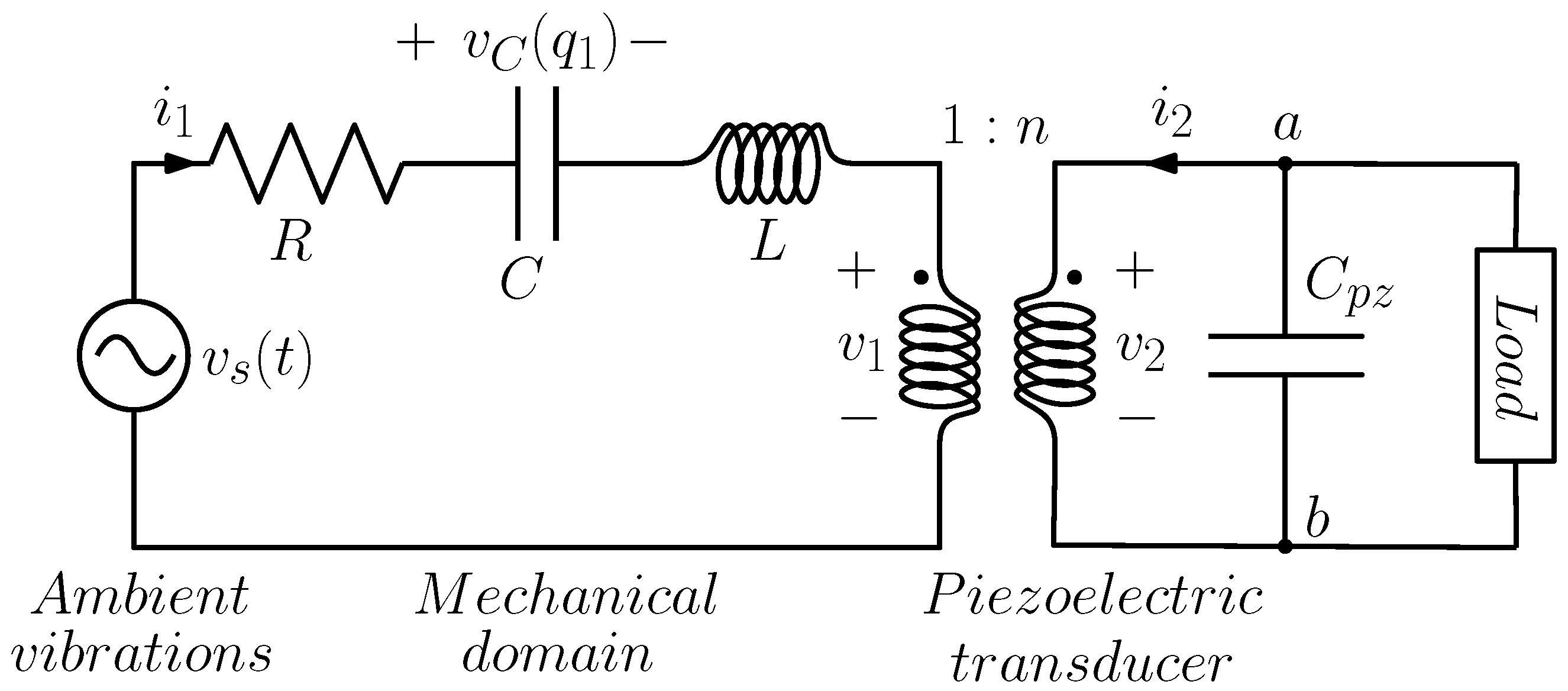
2. Piezoelectric Energy Harvester Modeling

A cantilever piezoelectric energy harvester for ambient mechanical vibration scavenging is composed of three main parts: A mechanical structure designed to capture the kinetic energy of parasitic mechanical vibrations; a piezoelectric transducer, responsible for the mechanical-to-electrical energy conversion, and an electrical domain for electric energy storage or electric power supply.

A schematic representation of a cantilever piezoelectric energy harvester is shown in Figure 1. The mechanical structure is composed of a cantilever beam fixed at one end to a moving support, with an inertial mass m placed at the opposite end, to increase the oscillation amplitude. The piezoelectric transducer is represented by a layer of piezoelectric material covering the beam. Vibrations of the support produce oscillations of the cantilever, inducing mechanical stress and strain in the piezoelectric material that are, in turn, converted into electrical current by the transducer. Finally, the electrical current is used to recharge, or supply power to an electrical load.

The piezoelectric transducer is considered, first. The constitutive equations for a linear piezoelectric material are [28]:

$$\left[\begin{array}{c}\mathit{S}\\ \mathit{D}\end{array}\right]=\left[\begin{array}{cc}{\mathbf{s}}^{\mathit{E}}& \mathit{d}\\ {\mathit{d}}_t& {\mathit{\epsilon }}^{\mathit{T}}\end{array}\right]\left[\begin{array}{c}\mathit{T}\\ \mathit{E}\end{array}\right],$$

(1)

where the rank two tensors $\mathit{S}$ and $\mathit{T}$ are the mechanical strain and stress, respectively, while the rank one tensors $\mathit{D}$ and $\mathit{E}$ are the dielectric charge displacement and electric field strength, respectively. ${\mathbf{s}}^{\mathit{E}}$ is the compliance tensor, under the condition of a constant electric field defined as strain generated per unit stress. The rank one tensor $\mathit{d}$ is the piezoelectric charge constants; finally ${\mathit{\epsilon }}^{\mathit{T}}$ is the absolute permittivity, e.g., the dielectric displacement per unit electric field for constant stress [29].

The linear Equation (1) describe the behavior of the piezoelectric material on a local scale, in terms of mechanical stress and strain, electric charge displacement and electrical field strength. A lumped parameter model can be derived in terms of global state variables, e.g., forces, displacements, currents and voltages, through spatial integration of the local variables. If the stiffness of the piezoelectric layer is neglected, the governing equations in the quasi-static regime are:

$$\begin{array}{cc}\hfill F_{pz}& =-\alpha e,\hfill \end{array}$$

(2)

$$\begin{array}{cc}\hfill q& =\alpha x-C_{pz}e,\hfill \end{array}$$

(3)

where $F_{pz}$ is the force applied on the mechanical part due to the electrical domain, x is the displacement, q is the electrical charge and e is the voltage. Concerning parameters, $\alpha$ is the electro-mechanical coupling (in N/V or As/m), and $C_{pz}$ is the electrical capacitance of the mechanical unconstrained system.

The governing equations in the mechanical domain can be derived from the mechanical Lagrangian function:

$${\mathcal{L}}_m(x,\dot{x})=K_m\left(\dot{x}\right)-U_m\left(x\right)={\displaystyle \frac{1}{2}}m{\dot{x}}^2-U_m\left(x\right),$$

(4)

where $K_m\left(\dot{x}\right)$ and $U_m\left(x\right)$ are the kinetic energy and the elastic potential, respectively, and the dot represents the time derivative. Introducing the mechanical dissipation function $D_m\left(\dot{x}\right)=\frac{1}{2}\gamma {\dot{x}}^2$, where $\gamma$ is the damping coefficient, and denoting by $f_m\left(t\right)$ the resultant of external forces acting on the mechanical domain, the Lagrange equation of motion is:

$${\displaystyle \frac{d}{dt}}{\displaystyle \frac{\partial {\mathcal{L}}_m(x,\dot{x})}{\partial \dot{x}}}-{\displaystyle \frac{\partial {\mathcal{L}}_m(x,\dot{x})}{\partial x}}+{\displaystyle \frac{\partial D_m\left(\dot{x}\right)}{\partial \dot{x}}}=F_{pz}+f_m.$$

(5)

Taking into account (2) and (4), the equation of motion reads:

$$m\ddot{x}+U^{\prime }\left(x\right)+\gamma \dot{x}=f_m\left(t\right)-\alpha e.$$

(6)

According to electrical-mechanical analogies, e.g., the impedance analogy, masses are replaced by inductances, elastic potentials by capacitors (for a linear elastic force with stiffness constant k, the substitution $k\to 1/C$ is made), damping by resistors, coordinates by charges, and forces by voltages. Thus, the following substitutions are used: $m\to L$, $x\to q_1$, $\dot{x}\to {\dot{q}}_1=i_1$, $\gamma \to R$, $f_m\left(t\right)\to v_s\left(t\right)$. Finally, Equation (6) is rewritten as a system of first order differential equations

$$\begin{array}{cc}\hfill {\displaystyle \frac{d{q}_1}{dt}}=& i_1\hfill \end{array}$$

(7)

$$\begin{array}{cc}\hfill {\displaystyle \frac{d{i}_1}{dt}}=& -{\displaystyle \frac{1}{L}}{U}^{\prime }\left(q_1\right)-{\displaystyle \frac{R}{L}}{i}_1-{\displaystyle \frac{1}{nL}}{v}_2+{\displaystyle \frac{v_s}{L}}\hfill \end{array}$$

(8)

where $n={\alpha }^{-1}$ and $v_2\left(t\right)=e\left(t\right)$. Figure 2 shows the equivalent circuit corresponding to Equations (7) and (8), feeding a generic load. The voltage across capacitor C is $v_C\left(q_1\right)=U^{\prime }\left(q_1\right)$.

3. Linear Harvester, Impedance Matching and Maximum Power Transfer

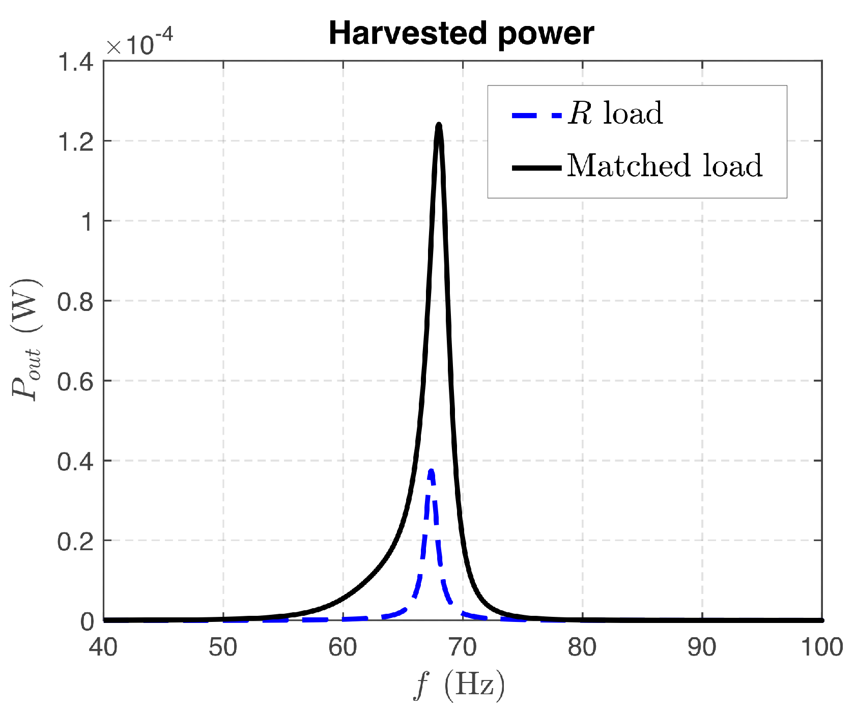
Ambient mechanical vibrations are random in nature, thus they are better described as stochastic processes. According to the Karhunen–Loéve theorem, a stochastic process can be represented as an infinite linear combination of orthogonal functions, in full analogy, for instance, to the Fourier series representation of a function on a bounded interval [30]. In many practical cases, the basis functions can be chosen to be sinusoidal, and the infinite sum is truncated to a suitable number of terms. From a circuit standpoint, such an external forcing can be represented as a series connection of sinusoidal voltage generators, and the linear system can be described using frequency domain analysis.

A quadratic elastic potential $U\left(x\right)=\frac{1}{2}k{x}^2$ yields a linear elastic force $F=-kx$ that, according to the mechanical-electrical analogy, is represented by a linear capacitor according to $k\to 1/C$, and by the voltage-charge characteristic $v_C=q_1/C$. If the load is also composed by linear two-terminal elements, the energy harvester is linear.

3.1. Resistive Load

Consider first the case when the load is a linear resistor with resistance $R_L$, see Figure 3a. At steady state, in the frequency domain, the governing equations for the circuit in Figure 2 are:

$$\left[\begin{array}{cc}R+jX\left(\omega \right)& {\displaystyle \frac{1}{n}}\\ -{\displaystyle \frac{1}{n}}& j\omega C_{pz}+G_L\end{array}\right]\left[\begin{array}{c}{\widehat{I}}_1\\ {\widehat{V}}_o\end{array}\right]=\left[\begin{array}{c}{\widehat{V}}_s\\ 0\end{array}\right],$$

(9)

where $j=\sqrt{-1}$, $X\left(\omega \right)=\omega L-1/\left(\omega C\right)$ is the left loop reactance, symbol $\widehat{F}$ denotes the phasor of the function $f\left(t\right)$, i.e., $f\left(t\right)=\Re \left[\widehat{F}{e}^{j\omega t}\right]$, where $\Re [·]$ denotes real part, and $G_L=1/R_L$ is the load admittance. The relevant transfer functions are:

$$\begin{array}{cc}\hfill Y_{\mathrm{in}}\left(\omega \right)& ={\displaystyle \frac{{\widehat{I}}_1}{{\widehat{V}}_s}}={\displaystyle \frac{n^2\left(j\omega C_{pz}+G_L\right)}{n^2\left(R+jX\left(\omega \right)\right)(j\omega C_{pz}+G_L)+1}},\hfill \end{array}$$

(10)

$$\begin{array}{cc}\hfill H\left(\omega \right)& ={\displaystyle \frac{{\widehat{V}}_o}{{\widehat{V}}_s}}={\displaystyle \frac{n}{n^2\left(R+jX\left(\omega \right)\right)(j\omega C_{pz}+G_L)+1}}.\hfill \end{array}$$

(11)

The transfer functions allow to calculated the average power delivered by the source, along with the average power absorbed by the load:

$$\begin{array}{cc}\hfill P_{\mathrm{in}}\left(\omega \right)=& {\displaystyle \frac{1}{2}}\Re \left[{\widehat{V}}_s{\widehat{I}}_1^{★}\right]={\displaystyle \frac{1}{2}}\Re \left[Y_{\mathrm{in}}\left(\omega \right)\right]{\left|{\widehat{V}}_s\right|}^2,\hfill \end{array}$$

(12)

$$\begin{array}{cc}\hfill P_{\mathrm{out}}\left(\omega \right)=& {\displaystyle \frac{1}{2}}\Re \left[{\widehat{V}}_o{\widehat{I}}^{★}\right]={\displaystyle \frac{1}{2}}{G}_L|H\left(\omega \right){|}^2{\left|{\widehat{V}}_s\right|}^2,\hfill \end{array}$$

(13)

where ★ denotes complex conjugate. The power efficiency is the ratio of the average powers:

$$\eta \left(\omega \right)={\displaystyle \frac{P_{\mathrm{out}}\left(\omega \right)}{P_{\mathrm{in}}\left(\omega \right)}}={\displaystyle \frac{{\left|H\left(\omega \right)\right|}^2}{\Re \left[Y_{\mathrm{in}}\left(\omega \right)\right]}}{G}_L.$$

(14)

3.2. Matched Load

A fundamental problem in energy harvesting is designing systems capable of harvesting the maximum power available from the surrounding environment. The maximum power transfer theorem states that, for a linear circuit, maximum power is transferred from the source to a load, if the load is matched to the rest of the circuit, meaning that the load impedance $Z_L$ must be the complex conjugate of the impedance seen at the load terminals. In practical applications, the load is determined a priori, and cannot be chosen at will by the designer. Consequently, the mechanical part and the piezoelectric transducer must be designed and realized with great care, to ensure that their impedance is matched to the load, a condition that is very difficult to attain in practice.

As an alternative, impedance matching can be obtained by interposing a two port matching network between the load and the rest of the circuit. Perfect matching can be obtained only at one specific frequency, and the matching network must be composed of lossless elements, in order not to dissipate power and, thus, to avoid reducing the harvester performance.

There are different realizations of matching networks, which differ for the number of components and for their topology. The simplest matching network is the L-network, requiring two reactive components only (inductor and capacitor), arranged to form an L structure. In general, depending on the problem under investigation, there are eight different possible arrangements. Here, we shall consider only one of them, whose choice is dictated by the problem under consideration.

Consider the equivalent circuit shown in Figure 2. The Thevenin equivalent circuit at nodes $a,b$ is composed by a voltage source:

$${\widehat{V}}_{\mathrm{eq}}\left(\omega \right)={\displaystyle \frac{n}{1+j\omega C_{pz}{n}^2(R+jX\left(\omega \right))}}{\widehat{V}}_s,$$

(15)

and by the equivalent impedance:

$$Z_{\mathrm{eq}}\left(\omega \right)={\displaystyle \frac{n^2(R+jX\left(\omega \right))}{1+j\omega C_{pz}{n}^2(R+jX\left(\omega \right))}}.$$

(16)

Let $R_{\mathrm{eq}}\left(\omega \right)=\Re \left[Z_{\mathrm{eq}}\left(\omega \right)\right]$ and $X_{\mathrm{eq}}\left(\omega \right)=\Im \left[Z_{\mathrm{eq}}\left(\omega \right)\right]$, where $\Im [·]$ denotes the imaginary part, and let ${\omega }_m$ be the angular frequency at which matching is desired. We shall assume $R_{\mathrm{eq}}\left({\omega }_m\right)<R_L$, consequently the matching network requires a shunt reactance to be placed in parallel with $R_L$. Considering that the energy of random mechanical vibrations is concentrated at low frequencies, it seems appropriate to chose a low-pass matching network, as shown in Figure 3b (The remaining seven possible arrangements for a L-matching network, including the case of high pass matching network, and the case $R_{\mathrm{eq}}\left({\omega }_m\right)>R_L$ which requires a shunt reactance placed in parallel with the Thevenin equivalent circuit, are not considered here).

The reactive part of $Z_{\mathrm{eq}}\left(\omega \right)$ can be matched introducing a reactance $X_{rs}\left(\omega \right)$ (the reactance of the two-terminal element $b_{rs}$ in Figure 3b), that resonates with $X_{\mathrm{eq}}\left(\omega \right)$ at the desired frequency ${\omega }_m$. If $X_{\mathrm{eq}}\left({\omega }_m\right)\le 0$, resonance is achieved by placing an inductor in series with $Z_{\mathrm{eq}}\left(\omega \right)$ such that:

$$L_{rs}={\displaystyle \frac{|X_{\mathrm{eq}}\left({\omega }_m\right)|}{{\omega }_m}}.$$

(17)

Conversely, if $X_{\mathrm{eq}}\left({\omega }_m\right)>0$, resonance is obtained with a capacitor such that:

$$C_{rs}={\displaystyle \frac{1}{{\omega }_m\left|X_{\mathrm{eq}}\left({\omega }_m\right)\right|}}.$$

(18)

The quality factor of the matching network is:

$$Q\left({\omega }_m\right)=\sqrt{{\displaystyle \frac{R_L}{R_{\mathrm{eq}}\left({\omega }_m\right)}}-1}.$$

(19)

The matching reactances are:

$$\begin{array}{cc}\hfill |{\overline{X}}_S|=& Q\left({\omega }_m\right)R_{\mathrm{eq}}\left({\omega }_m\right),\hfill \end{array}$$

(20)

$$\begin{array}{cc}\hfill |{\overline{X}}_P|=& {\displaystyle \frac{R_L}{Q\left({\omega }_m\right)}},\hfill \end{array}$$

(21)

and the matching components’ values are:

$$L_S={\displaystyle \frac{|{\overline{X}}_S|}{{\omega }_m}},C_P={\displaystyle \frac{1}{{\omega }_m\left|{\overline{X}}_P\right|}}.$$

(22)

Denoting by $X_{pz}\left(\omega \right)=-1/\left(\omega C_{pz}\right)$, $X_S\left(\omega \right)=\omega L_S$ and $X_P\left(\omega \right)=-1/\left(\omega C_P\right)$, the state equations are (explicit dependence on $\omega$ in the reactances is omitted for notation simplicity):

$$\left[\begin{array}{cc}R+jX& {\displaystyle \frac{j(X_{rs}+X_S)+j{X}_P\left|\right|R_L}{n\left(j{X}_P\right|\left|R_L\right)}}\\ -{\displaystyle \frac{1}{n}}& {\displaystyle \frac{j(X_{rs}+X_S+X_{pz})+j{X}_P\left|\right|R_L}{j{X}_{pz}(j{X}_P\left|\right|R_L)}}\end{array}\right]\left[\begin{array}{c}{\widehat{I}}_1\\ {\widehat{V}}_o\end{array}\right]=\left[\begin{array}{c}{\widehat{V}}_s\\ 0\end{array}\right],$$

(23)

where:

$$j{X}_P\left(\omega \right)\left|\right|R_L={\displaystyle \frac{j{X}_P\left(\omega \right)R_L}{j{X}_P\left(\omega \right)+R_L}}.$$

(24)

Let $\mathrm{\Delta }\left(\omega \right)$ be the determinant of the matrix above, the relevant transfer functions read:

$$\begin{array}{cc}\hfill Y_{\mathrm{in}}\left(\omega \right)=& {\displaystyle \frac{1}{\mathrm{\Delta }\left(\omega \right)}}{\displaystyle \frac{j(X_{rs}+X_S+X_{pz})+j{X}_P\left|\right|R_L}{j{X}_{pz}(j{X}_P\left|\right|R_L)}},\hfill \end{array}$$

(25)

$$\begin{array}{cc}\hfill H\left(\omega \right)=& {\displaystyle \frac{1}{n\mathrm{\Delta }\left(\omega \right)}},\hfill \end{array}$$

(26)

which permit calculating the average injected and collected power, and the power efficiency using Equations (12)–(14). The maximum average power collected by the harvester is given by the well known formula:

$$P_{\max }={\displaystyle \frac{|{\widehat{V}}_{\mathrm{eq}}\left({\omega }_m\right){|}^2}{8R_{\mathrm{eq}}\left({\omega }_m\right)}},$$

(27)

with 50% efficiency. Higher efficiency can be obtained, but renouncing to collect the maximum available average power.

As an example, we analyzed the equivalent circuit shown in Figure 2, comparing the resistive load with the matched load. The values of the circuit components are those given in [31], where they were determined through experimental results and finite element analysis. They are summarized in

Table 1. Values of circuit components, based on [31].

Parameter	Value
R	6.9366 $\mathsf{\Omega }$
C	5.874 $\mathsf{\mu }$F
L	1 H
$C_{pz}$	80.08 nF
$R_L$	1 M$\mathsf{\Omega }$
n	37.4254
$|V_s|$	83.0 mV

.

Figure 4 shows the root mean square values of the input current and of the output voltage as functions of frequency $f=\omega /\left(2\pi \right)$, respectively, given by:

$$\begin{array}{c}\hfill i_{1,rms}={\displaystyle \frac{1}{\sqrt{2}}}|Y_{\mathrm{in}}\left(\omega \right)\left|\right|{\widehat{V}}_s\left(\omega \right)|,\end{array}$$

(28)

$$\begin{array}{c}\hfill v_{o,rms}={\displaystyle \frac{1}{\sqrt{2}}}\left|H\left(\omega \right)\right||{\widehat{V}}_s\left(\omega \right)|.\end{array}$$

(29)

The linear harvester model with a resistive load shows a resonant peak approximately at the frequency $f_0=68$ Hz. It is worth mentioning that this resonant frequency is uniquely determined by the mechanical part and by the piezoelectric transducer. Consequently, because maximum power is scavenged at the resonance frequency, the two following points are fundamental in practical applications: First, an a priori knowledge of the frequency at which the maximum power of mechanical parasitic vibrations is concentrated is mandatory. Second, the mechanical system and the piezoelectric transducer must be designed to match this frequency. Combined together, these points make each energy harvesting solution hardly flexible, and very oriented to a specific environment.

The matching network solution proposed in this work, not only improves the performance of the energy harvester at the matching frequency, but can also be adapted to different environments. In fact, the matching network can be designed to realize optimum power transfer at a specific frequency, according to the procedure outlined in Section 3.

Table 2. Values of the components of the matching network at different frequencies, calculated using (17) and (22). The large values of the inductances are a consequence of the normalization used for the electrical equivalent of the mechanical part, i.e., $L_1=1$ H.

Matching Frequency	${\mathit{L}}_{\mathit{rs}}$	${\mathit{L}}_{\mathit{S}}$	${\mathit{C}}_{\mathit{P}}$
50 Hz	112.5157 H	34.7505 H	291.53 nF
68 Hz	170.3708 H	447.9216 H	11.764 nF
80 Hz	55.4050 H	23.7563 H	166.58e nF
100 Hz	32.9385 H	6.4850 H	390.59 nF

shows the values for the components of the matching network at different frequencies, evaluated according to (17) and (22).

Figure 5 shows a comparison between the power scavenged by an harvester with a resistive load and with a matched load. The linear energy harvester behaves as a passband filter. It can be seen that the matched load not only increases the harvested power at the matching frequency $f_m$, but it also gives a wider passband, an effect that can be exploited in the case of multi-frequency inputs or when the forcing frequency does not coincide exactly with the matching frequency.

The power scavenged by a linear harvester, with matched loads calculated at different frequencies, is shown in Figure 6. Matching frequencies and matching network parameters are those in Table 2. As discussed above, the matching frequency can be chosen at will, giving the designer the possibility to adapt an energy harvester to different environments, where the energy of mechanical vibrations is concentrated at different frequencies, which may be significantly different from the harvester resonant peak. In this case, however, a reminiscence of the mechanical system resonant frequency is present in the curves in the form of secondary peaks close to 68 Hz (see the inset in Figure 6). Results also suggest that while there is no difference in the maximum harvested power, working at a frequency close to the resonant one offers a wider tolerance to frequency mismatch, represented by a wider passband.

Finally, Figure 7 shows the comparison of the power efficiency, given by (14), for the harvester with resistive load, compared with the matched load. The efficiency of the resistive load monotonically decreases as the frequency increases, and is rather low at the frequency corresponding to the maximum harvested power. Clearly, the matched load offers higher efficiency over a wide frequency interval, and in particular at the matching frequency. At low and high frequencies, the two curves are very close. At the matching frequency $f_m=68$ Hz, the power efficiency for the matched load is 50%, as expected, and a larger value can be attained at lower frequency, as usual giving up the maximum harvested power condition.

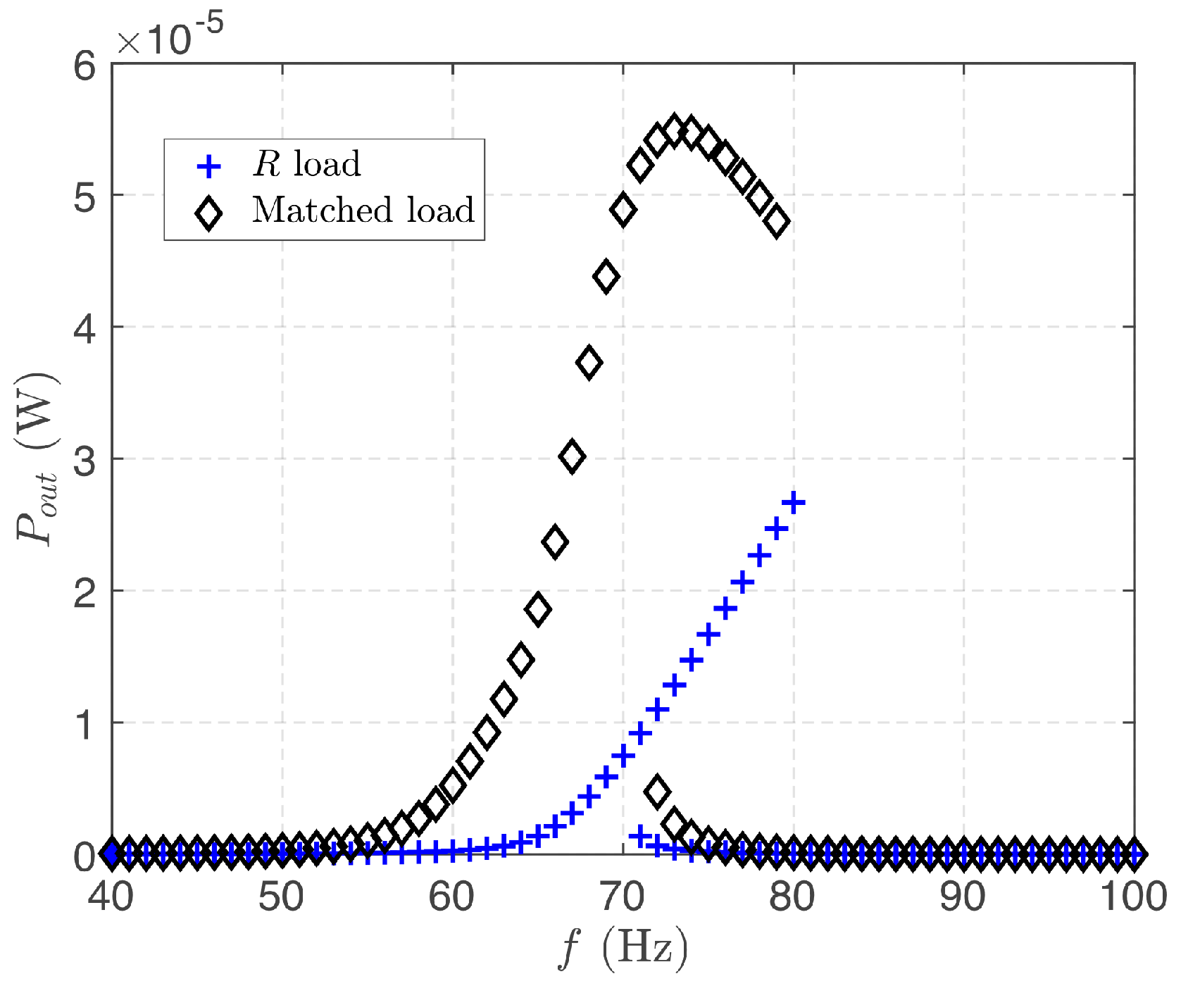
4. Nonlinear Energy Harvester Analysis

It is believed that, under certain circumstances, nonlinear energy harvesters may outperform linear ones, trading off the efficiency at the resonant frequency for a larger bandwidth. An energy harvester is nonlinear when nonlinear stiffness effects are taken into account, e.g., when the elastic potential of the beam takes the form $U\left(x\right)=a{x}^2+b{x}^4$, where a and b are real valued parameters. Consequently, the state Equations (7) and (8) for the equivalent circuit of Figure 2 must include a nonlinear capacitor with the nonlinear voltage-charge characteristic $U^{\prime }\left(q_1\right)=v_C=q_1/C+q_1^3/\tilde{C}$.

The analysis of nonlinear circuits and systems is nontrivial, and requires ad hoc techniques. Hereinafter, for the sake of simplicity we shall assume that the energy of mechanical vibrations is concentrated at a single frequency $f_0$, i.e., the voltage source $v_s\left(t\right)$ will be considered a simple periodic function with period $T_0$ and angular frequency ${\omega }_0=2\pi /T_0$. It is also worth mentioning that the theory for the design of nonlinear circuits is very limited; therefore, we shall apply the same matching network designed for the linear harvester also to the nonlinear system.

Concerning the analysis of the nonlinear circuit, the time domain state equations for the electrical part are also needed. Including the resistive load of Figure 3 into the equivalent circuit, and applying Kirchhoff current law to node a yields:

$${\displaystyle \frac{d{v}_2}{dt}}={\displaystyle \frac{1}{n{C}_{pz}}}{i}_1-{\displaystyle \frac{G_L}{C_{pz}}}{v}_2.$$

(30)

For the matched load, only the case where the two-terminal element $b_{rs}$ is an inductor with inductance $L_{rs}$ is considered here for the sake of simplicity. Applying Kirchhoff current and voltage laws yields:

$$\begin{array}{cc}\hfill {\displaystyle \frac{d{v}_2}{dt}}& ={\displaystyle \frac{1}{C_{pz}}}\left({\displaystyle \frac{i_1}{n}}-i\right),\hfill \end{array}$$

(31)

$$\begin{array}{cc}\hfill {\displaystyle \frac{d{v}_o}{dt}}& ={\displaystyle \frac{1}{C_P}}\left(i-G_L{v}_o\right),\hfill \end{array}$$

(32)

$$\begin{array}{cc}\hfill {\displaystyle \frac{di}{dt}}& ={\displaystyle \frac{1}{L_{rs}+L_S}}\left(v_2-v_o\right).\hfill \end{array}$$

(33)

Together with (7) and (8), Equation (30) (respectively, (31)–(33)) describe the dynamic behavior of the nonlinear harvester with resistive (respectively, matched) load.

4.1. The Harmonic Balance Technique

Harmonic Balance (HB) is a powerful numerical technique commonly exploited in many scientific areas, including electronic engineering, to efficiently implement the direct determination of periodic or quasi-periodic solutions of dynamical systems, thus fully avoiding the computation of the transient part of the solution. Essentially, HB transforms the system differential equations into an algebraic system whose unknowns are the coefficients of the Fourier series representing the steady-state solution [32,33].

Let us initially consider a scalar, T-periodic real function $x\left(t\right)$. We represent the function in the frequency domain by means of a (truncated) exponential Fourier series:

$$x\left(t\right)=\sum _{h=-N_{\mathrm{H}}}^{N_{\mathrm{H}}}{\widehat{x}}_h{\mathrm{e}}^{{\displaystyle jh{\omega }_{0}t}},$$

(34)

where ${\widehat{x}}_h$ is the h-th harmonic amplitude, associated to the h-th harmonic at the (angular) frequency $h{\omega }_0=h2\pi /T$. As $x\left(t\right)$ is real, ${\widehat{x}}_{-h}={\widehat{x}}_h^{★}$, and therefore the Fourier series is completely defined by $2N_{\mathrm{H}}+1$ real coefficients. In terms of numerical implementation, a more effective approach to HB requires replacing (34) with a trigonometric series representation [34]. Nevertheless, we prefer to use the more compact exponential form for the sake of theoretical developments.

After discretizing the $[0,T]$ fundamental period with a set of $2N_{\mathrm{H}}+1$ time samples $t_k$ ($k=1,\dots ,2N_{\mathrm{H}}+1$), the samples of the time-dependent variable are collected into vector $\breve{\mathbf{x}}={[x\left(t_1\right),x\left(t_2\right),\dots ,x\left(t_{2N_{\mathrm{H}}+1}\right)]}^{\mathrm{T}}$ (${}^{\mathrm{T}}$ denotes the transpose), which is related to the collection of harmonic amplitudes $\widehat{\mathbf{x}}={[{\widehat{x}}_{-N_{\mathrm{H}}},{\widehat{x}}_{-N_{\mathrm{H}}+1},\dots ,{\widehat{x}}_0,\dots ,{\widehat{x}}_{N_{\mathrm{H}}}]}^{\mathrm{T}}$ by means of the discrete Fourier transform (DFT) invertible linear operator ${\mathrm{\Gamma }}^{-1}$:

$$\breve{\mathbf{x}}={\mathrm{\Gamma }}^{-1}\widehat{\mathbf{x}}⟺\widehat{\mathbf{x}}=\mathrm{\Gamma }\breve{\mathbf{x}}.$$

(35)

${\mathrm{\Gamma }}^{-1}$ is the approximate matrix representation of the operator defining the Fourier series development of a T-periodic function.

In the frequency domain, for the exponential series a diagonal complex matrix $\mathsf{\Omega }$ of size $(2N_{\mathrm{H}}+1)\times (2N_{\mathrm{H}}+1)$ proportional to ${\omega }_0$, represents the time derivative [32]:

$$\widehat{\dot{\mathbf{x}}}=\mathrm{\Gamma }\breve{\dot{\mathbf{x}}}=\mathsf{\Omega }\widehat{\mathbf{x}}.$$

(36)

Moving now to the vector case, considering that $\mathbf{x}\left(t\right)\in {\mathbb{R}}^n$ (35) and (36) are easily generalized by expanding each time sample $\alpha \left(t_i\right)$ into a vector $\mathbf{x}\left(t_i\right)\in {\mathbb{R}}^n$, whose collection becomes $\breve{\mathbf{x}}={[{\mathbf{x}}^{\mathrm{T}}\left(t_1\right),{\mathbf{x}}^{\mathrm{T}}\left(t_2\right),\dots ,{\mathbf{x}}^{\mathrm{T}}\left(t_{2N_{\mathrm{H}}+1}\right)]}^{\mathrm{T}}\in {\mathbb{R}}^{n(2N_{\mathrm{H}}+1)}$. Correspondingly, the frequency domain representation is $\widehat{\mathbf{x}}={[{\widehat{\mathbf{x}}}_{-N_{\mathrm{H}}}^{\mathrm{T}},\dots ,{\widehat{\mathbf{x}}}_0^{\mathrm{T}},\dots ,{\widehat{\mathbf{x}}}_{N_{\mathrm{H}}}^{\mathrm{T}}]}^{\mathrm{T}}\in {\mathbb{C}}^{n(2N_{\mathrm{H}}+1)}$. In this way, Equations (35) and (36) can formally be extended by defining two block diagonal matrixes ${\mathrm{\Gamma }}_n^{-1}$ and ${\mathsf{\Omega }}_n$ of size $n(2N_{\mathrm{H}}+1)\times n(2N_{\mathrm{H}}+1)$, where each diagonal block of size $(2N_{\mathrm{H}}+1)\times (2N_{\mathrm{H}}+1)$ is defined by the fundamental operators ${\mathrm{\Gamma }}^{-1}$ and $\mathsf{\Omega }$, respectively:

$$\breve{\mathbf{x}}={\mathrm{\Gamma }}_n^{-1}\widehat{\mathbf{x}},\widehat{\dot{\mathbf{x}}}={\mathsf{\Omega }}_n\widehat{\mathbf{x}}.$$

(37)

Let us now apply these concepts to the case of a vector dynamical system of size n, forced by a T-periodic source term $\mathbf{s}\left(t\right)$:

$$\dot{\mathbf{x}}\left(t\right)=\mathbf{f}\left(\mathbf{x}\left(t\right)\right)+\mathbf{s}\left(t\right).$$

(38)

After time-sampling and DFT transformation, (38) becomes:

$${\mathsf{\Omega }}_n\widehat{\mathbf{x}}=\widehat{\mathbf{f}}\left({\mathrm{\Gamma }}_n^{-1}\widehat{\mathit{x}}\right)+\widehat{\mathbf{s}},$$

(39)

where $\widehat{\mathbf{f}}$ represents the collection of harmonic amplitudes for the T-periodic function $\mathbf{f}\left(\mathbf{x}\right(t\left)\right)$.

Algebraic Equation (39) can be solved numerically exploiting the Newton algorithm, and specialized techniques have also been developed for specific analyses, such as the stability assessment of the resulting solution [34]. To introduce the stability analysis of the periodic solution ${\mathbf{x}}_{\mathrm{S}}\left(t\right)$, let us assume that such solution is slightly perturbed by a variation ${\mathbf{x}}_{\mathrm{p}}\left(t\right)$. The resulting variable $\mathbf{x}\left(t\right)={\mathbf{x}}_{\mathrm{S}}\left(t\right)+{\mathbf{x}}_{\mathrm{p}}\left(t\right)$ should satisfy (38). However, if the perturbation is a small variation of the periodic solution, we can linearize (38) obtaining a linear equation governing the evolution of ${\mathbf{x}}_{\mathrm{p}}\left(t\right)$:

$${\dot{\mathbf{x}}}_{\mathrm{p}}={\mathbf{J}}_{\mathbf{f}}\left(t\right){\mathbf{x}}_{\mathrm{p}}\left(t\right),$$

(40)

where ${\mathbf{J}}_{\mathbf{f}}\left(t\right)$ is a T-periodic matrix corresponding to the Jacobian of $\mathbf{f}$ evaluated in the periodic solution ${\mathbf{x}}_{\mathrm{S}}\left(t\right)$. The general solution of the linear, periodically time-varying system (40) is dictated by Floquet Theorem [34,35]:

$${\mathbf{x}}_{\mathrm{p}}\left(t\right)={\mathbf{u}}_k\left(t\right){\mathrm{e}}^{{\displaystyle {\mu }_{k}t}},$$

(41)

where ${\mathbf{u}}_k\left(t\right)$ are T-periodic functions called Floquet eigenvectors of the solution ${\mathbf{x}}_{\mathrm{S}}\left(t\right)$, while ${\mu }_k$ are scalar constants dubbed Floquet exponents. There are n independent Floquet eigenvectors (i.e., $k=1,\dots ,n$ in (41)), while the value of $\Re \left\{{\mu }_k\right\}$ determines the asymptotic properties of the perturbation: for the solution to be asymptotically stable, all Floquet exponents must have a negative real part. According to (41), however, for each ${\mu }_k$ an infinite set of equivalent exponents can be defined as a function of an integer parameter m [36]:

$${\mu }_k^{\left(m\right)}={\mu }_k+jm{\omega }_0,m\mathrm{integer}.$$

(42)

To resolve this redundancy, stability is usually verified checking the n Floquet multipliers ${\lambda }_k=exp\left({\mu }_k^{\left(m\right)}T\right)$. Three cases are possible: (1) if $|{\lambda }_k|<1$$\forall k=1,\dots ,n$, the solution ${\mathit{x}}_{\mathrm{S}}\left(t\right)$ is asymptotically stable (i.e., the perturbation converges to zero); (2) if $\exists k:|{\lambda }_k|>1$ the solution is unstable; (3) if $\exists k:|{\lambda }_k|=1$, the solution undergoes a bifurcation. In particular, ${\lambda }_k=1$ corresponds to a fold bifurcation, ${\lambda }_k=-1$ to a period doubling, while a unitary $|{\lambda }_k|$ with phase different from 0 or $\pi$ represents a Neimark-Sacker bifurcation with a spurious frequency arising at the imaginary part of ${\lambda }_k$ [36].

Substituting (41) into (40), the Floquet eigenvectors and eigenvalues are shown to satisfy:

$${\dot{\mathbf{u}}}_k\left(t\right)-{\mathbf{J}}_{\mathbf{f}}\left(t\right){\mathbf{u}}_k\left(t\right)={\mu }_k{\mathbf{u}}_k\left(t\right).$$

(43)

As the Floquet eigenvectors are T-periodic functions of time, the HB approach can also be exploited for the determination of the Floquet quantities [34]. After time-sampling and DFT transformation, (43) becomes an eigenvalue problem:

$$\left({\mathsf{\Omega }}_n-{\widehat{\mathbf{J}}}_{\mathbf{f}}\right){\widehat{\mathbf{u}}}_k={\mu }_k{\widehat{\mathbf{u}}}_k,$$

(44)

where ${\widehat{\mathbf{J}}}_{\mathbf{f}}={\mathrm{\Gamma }}_n{\breve{\mathbf{J}}}_{\mathbf{f}}{\mathrm{\Gamma }}_n^{-1}$, ${\breve{\mathbf{J}}}_{\mathbf{f}}$ being the block diagonal matrix built expanding each element of ${\mathbf{J}}_{\mathbf{f}}\left(t\right)$ into the diagonal matrix of the corresponding time samples. The numerical determination of the Floquet eigenvectors and eigenvalues is in some cases rather delicate, and specialized techniques have been specifically devised to overcome the main implementation issues [37,38].

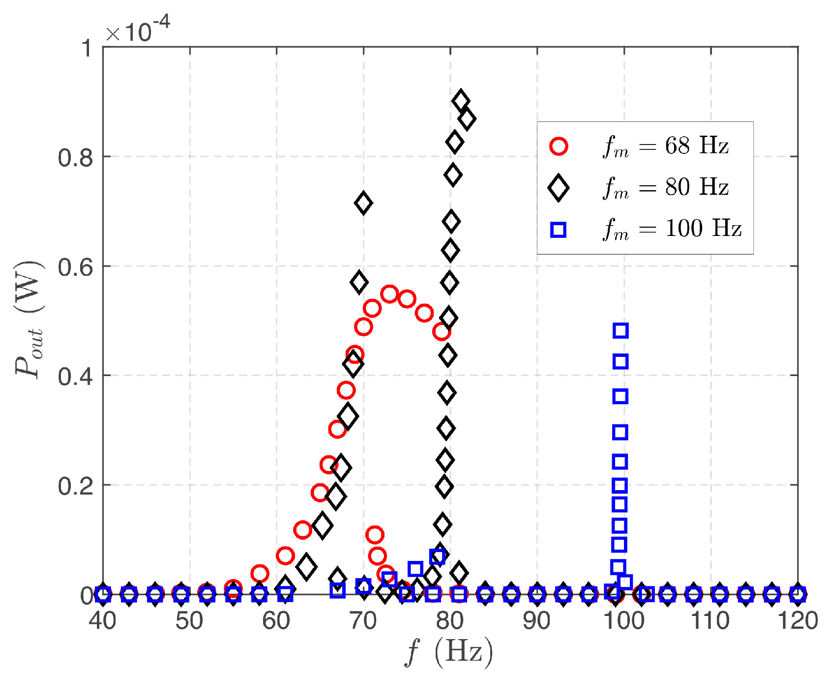
4.2. Nonlinear Piezoelectric Energy Harvester Analysis

The HB technique wasapplied to analyze the nonlinear energy harvester described by the differential system (7) and (8), including the cubic approximation of the voltage-charge relation in the equivalent representation of the mechanical system, and (30) (respectively (31)–(33)). For our analysis, we considered $\tilde{C}=0.005$ pF to introduce a significant nonlinearity. To speed up the numerical procedure, the HB technique was applied in conjunction with a continuation method, where the solution for a certain value of a prescribed parameter and of the forcing frequency is used as the initial condition for the Newton algorithm applied to the following value of the parameter. Notice that a main advantage of the HB technique is that it allows for the detection of both stable and unstable solutions, including limit cycles of saddle type that cannot be detected through numerical time-integration, neither forward nor backward in time. In the following results, we considered $N_{\mathrm{H}}=100$ harmonics.

Figure 8 shows the root mean square values (rms) for the input current and the output voltage, presented as a function of the forcing frequency. It can be seen that the system with both load types exhibits the same qualitative behavior. For small value of f, there is a unique, asymptotically stable periodic solution (blue crosses are for the resistive load, and black squares are for the matched load, respectively). As the forcing frequency is increased, the rms values increase, implying that the amplitude of the periodic solution increases. At the critical value $f_{\mathrm{SN}{}_1}\approx 71$ Hz, a saddle node bifurcation, identified by a Floquet multiplier equal to one, occurs. Two new periodic solutions emerge: the smaller is asymptotically stable (blue × symbols are for the resistive load, black circles are for the matched load), whereas the larger is unstable of saddle type (red pentagrams are for the resistive load, red diamonds are for the matched load). At the critical frequency $f_{\mathrm{SN}{}_2}\approx 81$ Hz, the unstable solution and the large, stable periodic solution collide, and disappear through a second saddle-node bifurcation. The small, stable limit cycle remains as the unique solution. With regard to the input current, there are no significant differences for the two load types. Conversely, the output voltage is significantly greater for the matched load over a wide frequency interval, but especially at the matching frequency $f_0=68$ Hz.

The rms values of $i_1$ and $v_o$ allow for an easy calculation of the average injected and extracted power. From Figure 3, the average power transferred to the load is:

$$P_{\mathrm{out}}={\displaystyle \frac{G_L}{T}}{\int }_0^T{v}_o{\left(t\right)}^2\mathrm{d}t=G{v}_{o,rms}^2.$$

(45)

For the input power, using Tellegen’s theorem, we have:

$$P_{\mathrm{in}}={\displaystyle \frac{1}{T}}{\int }_0^T{v}_s\left(t\right)i_1\left(t\right)dt=R{i}_{1,rms}^2+G_L{v}_{o,rms}^2,$$

(46)

where we used the fact that the transformer does not dissipate power, as it only transfers power from the left loop to the right branches, and that reactive elements (inductors and capacitors) do not absorb active power, being able to handle reactive power only.

Figure 9 shows the average power absorbed by the load for the resistive load (blue crosses) and the matched load (black diamonds) as functions of the forcing frequency. The matching network is calculated at $f_m=68$ Hz. It is evident that the matched load outperforms the resistive load over a wide frequency band. It is also worth mentioning that the introduction of even a comparatively small nonlinearity, results in a significant shift of the frequency at which the harvester with resistive load provides the maximum average output power. Therefore, if nonlinearity is not properly taken into account, the harvester average output power will be significantly lower than expected. The frequency shift in the peak power is also present for the harvester with matched load, although much less noticeable, and the maximum average output power remains quite close to the matching frequency.

Figure 10 shows the power efficiency as a function of the forcing frequency. The matched load offers higher efficiency with respect to the resistive load over a wide frequency range. More importantly, in close similarity to the linear case, for the resistive load the efficiency is a monotonically decreasing function of frequency, and it becomes particularly low at the resonant frequency $f_0$. Conversely, for the matched load the efficiency is equal to 50% at the matching frequency of 68 Hz, as expected, and remains relatively high around that frequency.

Finally, Figure 11 shows the harvested power versus the forcing frequency for a nonlinear energy harvester with matching network, designed at the three different frequencies 68 Hz, 80 Hz and 100 Hz. The values of the components for each matching network are listed in Table 2. It can be seen that also for the nonlinear harvester, the matching network allows selecting the frequency at which maximum power is harvested.

5. Conclusions

Parasitic ambient mechanical vibrations are a viable energy source, which can be converted into electrical energy exploiting a piezoelectric transducer, and thus they can be used as a power source for electronic circuits, sensors and actuators. Limiting key factors are the relatively low power density of mechanical vibrations, and the impedance mismatch between mechanical and electrical domains.

In this work, a possible solution to the aforementioned limitations is proposed. We analyzed a piezoelectric energy harvester for parasitic mechanical vibrations, subject to an external force. The differential equations for the mechanical part have been derived from Lagrangian mechanics, and those for the piezoelectric transducer from the properties of piezoelectric materials. Starting from these differential equations, an equivalent circuit model was devised exploiting mechanical-to-electrical analogies.

The equivalent circuit is instrumental in designing a matching network that maximizes the power transfer from the harvester to the electrical load. The matching network achieves impedance matching at a specific frequency, for any a priori fixed value of the load resistance. The matching frequency can be chosen at will by the designer and does not need to coincide with the resonant frequency of the harvester. Moreover with the matching network, maximum power transfer and the well know 50% power efficiency are obtained at the same frequency. By contrast, for a resistive load the power efficiency decreases as the frequency increases.

The matching network also increases the harvested power over a wide frequency bandwidth. According to our simulations, with respect to a simple resistive load, the maximum harvested power is increased more than three times, while the total harvested power over the whole frequency spectrum is increased more than six times. These values can be regarded as an upper bound, as a real matching network will of course be plagued by losses that may slightly reduce the harvested power gain.

The frequency bandwidth can be further extended considering a nonlinear energy harvester. It is shown that the nonlinear differential equations describing the harvester dynamics can be efficiently analyzed applying a frequency domain technique, namely harmonic balance. The occurrence of nonlinear resonance and bifurcation phenomena are illustrated and analyzed. Although there is little theory for the design of nonlinear circuits and systems, the matching network designed for the linear harvester improves the maximum harvested power, power bandwidth and power efficiency also for the nonlinear case.

References

1. Roundy, S.; Wright, P.K.; Rabaey, J.M. Energy Scavenging for Wireless Sensor Networks; Springer: Boston, MA, USA, 2003. [Google Scholar]
2. Paradiso, J.A.; Starner, T. Energy scavenging for mobile and wireless electronics. IEEE Pervasive Comput. 2005, 4, 18–27. [Google Scholar] [CrossRef]
3. Beeby, S.P.; Tudor, M.J.; White, N. Energy harvesting vibration sources for microsystems applications. Meas. Sci. Technol. 2006, 17, R175. [Google Scholar] [CrossRef]
4. Mitcheson, P.; Yeatman, E.; Rao, G.; Holmes, A.; Green, T. Energy Harvesting From Human and Machine Motion for Wireless Electronic Devices. Proc. IEEE 2008, 96, 1457–1486. [Google Scholar] [CrossRef] [Green Version]
5. Lu, X.; Wang, P.; Niyato, D.; Kim, D.I.; Han, Z. Wireless Networks with RF Energy Harvesting: A Contemporary Survey. IEEE Commun. Surv. Tutor. 2015, 17, 757–789. [Google Scholar] [CrossRef] [Green Version]
6. Khaligh, A.; Zeng, P.; Zheng, C. Kinetic energy harvesting using piezoelectric and electromagnetic technologies—State of the art. IEEE Trans. Ind. Electron. 2009, 57, 850–860. [Google Scholar] [CrossRef]
7. Vocca, H.; Neri, I.; Travasso, F.; Gammaitoni, L. Kinetic energy harvesting with bistable oscillators. Appl. Energy 2012, 97, 771–776. [Google Scholar] [CrossRef]
8. Wen, X.; Yang, W.; Jing, Q.; Wang, Z.L. Harvesting broadband kinetic impact energy from mechanical triggering/vibration and water waves. ACS Nano 2014, 8, 7405–7412. [Google Scholar] [CrossRef]
9. Fu, Y.; Ouyang, H.; Davis, R.B. Nonlinear dynamics and triboelectric energy harvesting from a three-degree-of-freedom vibro-impact oscillator. Nonlinear Dyn. 2018, 92, 1985–2004. [Google Scholar] [CrossRef]
10. Shin, Y.H.; Choi, J.; Kim, S.J.; Kim, S.; Maurya, D.; Sung, T.H.; Priya, S.; Kang, C.Y.; Song, H.C. Automatic resonance tuning mechanism for ultra-wide bandwidth mechanical energy harvesting. Nano Energy 2020, 77, 104986. [Google Scholar] [CrossRef]
11. Wang, Z.; Du, Y.; Li, T.; Yan, Z.; Tan, T. A flute-inspired broadband piezoelectric vibration energy harvesting device with mechanical intelligent design. Appl. Energy 2021, 303, 117577. [Google Scholar] [CrossRef]
12. Cottone, F.; Vocca, H.; Gammaitoni, L. Nonlinear energy harvesting. Phys. Rev. Lett. 2009, 102, 080601. [Google Scholar] [CrossRef] [PubMed] [Green Version]
13. Gammaitoni, L.; Neri, I.; Vocca, H. Nonlinear oscillators for vibration energy harvesting. Appl. Phys. Lett. 2009, 94, 164102. [Google Scholar] [CrossRef] [Green Version]
14. Mann, B.P.; Sims, N.D. Energy harvesting from the nonlinear oscillations of magnetic levitation. J. Sound Vib. 2009, 319, 515–530. [Google Scholar] [CrossRef] [Green Version]
15. Gammaitoni, L.; Neri, I.; Vocca, H. The benefits of noise and nonlinearity: Extracting energy from random vibrations. Chem. Phys. 2010, 375, 435–438. [Google Scholar] [CrossRef]
16. Daqaq, M.F. Response of uni-modal Duffing-type harvesters to random forced excitations. J. Sound Vib. 2010, 329, 3621–3631. [Google Scholar] [CrossRef]
17. Bonnin, M.; Traversa, F.L.; Bonani, F. Analysis of influence of nonlinearities and noise correlation time in a single-DOF energy-harvesting system via power balance description. Nonlinear Dyn. 2020, 100, 119–133. [Google Scholar] [CrossRef]
18. Daqaq, M.F. On intentional introduction of stiffness nonlinearities for energy harvesting under white Gaussian excitations. Nonlinear Dyn. 2012, 69, 1063–1079. [Google Scholar] [CrossRef]
19. Xu, M.; Li, X. Two-step approximation procedure for random analyses of tristable vibration energy harvesting systems. Nonlinear Dyn. 2019, 98, 2053–2066. [Google Scholar] [CrossRef]
20. Daqaq, M.F.; Crespo, R.S.; Ha, S. On the efficacy of charging a battery using a chaotic energy harvester. Nonlinear Dyn. 2020, 99, 1525–1537. [Google Scholar] [CrossRef]
21. Yan, Z.; Sun, W.; Hajj, M.R.; Zhang, W.; Tan, T. Ultra-broadband piezoelectric energy harvesting via bistable multi-hardening and multi-softening. Nonlinear Dyn. 2020, 100, 1057–1077. [Google Scholar] [CrossRef]
22. Bonnin, M.; Traversa, F.L.; Bonani, F. On the application of circuit theory and nonlinear dynamics to the design of highly efficient energy harvesting systems. In Proceedings of the 2021 International Conference on Smart Energy Systems and Technologies (SEST), Vaasa, Finland, 6–8 September 2021. [Google Scholar] [CrossRef]
23. Brufau-Penella, J.; Puig-Vidal, M. Piezoelectric energy harvesting improvement with complex conjugate impedance matching. J. Intell. Mater. Syst. Struct. 2009, 20, 597–608. [Google Scholar] [CrossRef]
24. Abdelmoula, H.; Abdelkefi, A. Ultra-wide bandwidth improvement of piezoelectric energy harvesters through electrical inductance coupling. Eur. Phys. J. Spec. Top. 2015, 224, 2733–2753. [Google Scholar] [CrossRef]
25. Huang, D.; Zhou, S.; Litak, G. Analytical analysis of the vibrational tristable energy harvester with a RL resonant circuit. Nonlinear Dyn. 2019, 97, 663–677. [Google Scholar] [CrossRef]
26. Yu, T.; Zhou, S. Performance investigations of nonlinear piezoelectric energy harvesters with a resonant circuit under white Gaussian noises. Nonlinear Dyn. 2021, 103, 183–196. [Google Scholar] [CrossRef]
27. Bonnin, M.; Traversa, F.L.; Bonani, F. Leveraging circuit theory and nonlinear dynamics for the efficiency improvement of energy harvesting. Nonlinear Dyn. 2021, 104, 367–382. [Google Scholar] [CrossRef]
28. IEEE Std 1859-2017; IEEE Standard on Piezoelectricity. IEEE: Minneapolis, MN, USA, 1988. [CrossRef]
29. Priya, S.; Inman, D.J. Energy Harvesting Technologies; Springer: Boston, MA, USA, 2009; Volume 21. [Google Scholar]
30. Ghanem, R.G.; Spanos, P.D. Stochastic Finite Elements: A Spectral Approach; Courier Corporation: North Chelmsford, MA, USA, 2003. [Google Scholar]
31. Yang, Y.; Tang, L. Equivalent circuit modeling of piezoelectric energy harvesters. J. Intell. Mater. Syst. Struct. 2009, 20, 2223–2235. [Google Scholar] [CrossRef]
32. Kundert, K.S.; Sangiovanni-Vincentelli, A.L.; White, J.K. Steady-State Methods for Simulating Analog and Microwave Circuits; Springer: Boston, MA, USA, 2010. [Google Scholar]
33. Bonnin, M.; Traversa, F.; Bonani, F. Efficient spectral domain technique for the frequency locking analysis of nonlinear oscillators. Eur. Phys. J. Plus 2018, 133, 246. [Google Scholar] [CrossRef]
34. Traversa, F.L.; Bonani, F.; Donati Guerrieri, S. A frequency-domain approach to the analysis of stability and bifurcations in nonlinear systems described by differential-algebraic equations. Int. J. Circuit Theory Appl. 2008, 36, 421–439. [Google Scholar] [CrossRef] [Green Version]
35. Farkas, M. Periodic Motions; Springer Nature: New York, NY, USA, 1994. [Google Scholar]
36. Cappelluti, F.; Traversa, F.L.; Bonani, F.; Donati Guerrieri, S.; Ghione, G. Large-Signal Stability of Symmetric Multibranch Power Amplifiers Exploiting Floquet Analysis. IEEE Trans. Microw. Theory Tech. 2013, 61, 1580–1587. [Google Scholar] [CrossRef]
37. Traversa, F.; Bonani, F. Frequency-domain evaluation of the adjoint Floquet eigenvectors for oscillator noise characterisation. IET Circuits Devices Syst. 2011, 5, 46. [Google Scholar] [CrossRef] [Green Version]
38. Traversa, F.L.; Bonani, F. Improved harmonic balance implementation of Floquet analysis for nonlinear circuit simulation. AEU Int. J. Electron. Commun. 2012, 66, 357–363. [Google Scholar] [CrossRef] [Green Version]
Figure 1. Schematic representation of a piezoelectric energy harvester. From [22].
Energies 15 02764 g001
Figure 2. Equivalent circuit for a piezoelectric energy harvester. Notice that i 1 = q ˙ 1 .
Energies 15 02764 g002
Figure 3. The two types of load considered. (a): Resistive load. (b): Resistive load with a low-pass L-matching network. The two-terminal element b r s is a reactive component (inductor or capacitor, depending on the reactive part of the equivalent impedance seen on the left of v 2 ) designed to resonate with the harvester reactance.
Energies 15 02764 g003
Figure 4. Root mean square values for the input current (left) and the output voltage (right) for a linear harvester. Load matching is calculated at f 0 = 68 Hz.
Energies 15 02764 g004
Figure 5. Scavenged power vs. frequency for a linear harvester. Load matching calculated at f m = 68 Hz.
Energies 15 02764 g005
Figure 6. Scavenged power vs. frequency for a linear harvester with matched load, for different matching frequencies. Values of the components of the matching networks at each matching frequency are reported in Table 2.
Energies 15 02764 g006
Figure 7. Power efficiency vs. frequency for the resistive and the matched load. Load matching is calculated at f m = 68 Hz.
Energies 15 02764 g007
Figure 8. Root mean square values for the input current (left) and the output voltage (right) for a nonlinear harvester. Load matching is calculated at f 0 = 68 Hz. Blue crosses, blue × and red pentagrams are for the resistive load. Black squares, black circles and red diamonds are for the matched load. Blue and black markers refer to stable limit cycles, red markers are for unstable limit cycles.
Energies 15 02764 g008
Figure 9. Average output power vs. forcing frequency. Blue crosses are for the resistive load; black diamonds are for the matched load. Matching frequency is f m = 68 Hz.
Energies 15 02764 g009
Figure 10. Power efficiency vs. forcing frequency. Blue crosses are for the resistive load; black diamonds are for the matched load. Matching frequency is f 0 = 68 Hz.
Energies 15 02764 g010
Figure 11. Output average power vs. forcing frequency. The matched load is evaluated at three different matching frequencies. Values of the components of the matching network at each frequencies are reported in Table 2. Red circles refers to f m = 68 Hz, black diamonds to f m = 80 Hz, blue squares to f m = 100 Hz.
Energies 15 02764 g011