Article

Polar Voltage Space Vectors of the Six-Phase Two-Level VSI

Department of Ship Automation, Gdynia Maritime University, Poland Morska St. 83, 81-225 Gdynia, Poland
*
Author to whom correspondence should be addressed.
Energies 2022, 15(8), 2763; https://doi.org/10.3390/en15082763
Submission received: 27 February 2022 / Revised: 4 April 2022 / Accepted: 7 April 2022 / Published: 9 April 2022
(This article belongs to the Special Issue Power Quality and Electrical Machines)

Abstract

:
The paper recommends polar voltage space vectors of the six-phase and two-level inverter as a useful mathematical tool for vector control of the inverter. The inverter model is described using three mathematical tools: analytic expressions, voltage state, and space vectors. The analytic formulas allow for the determination of elementary physical inverter quantities: current and voltage. The state voltage vectors make it easy to define phase voltage distribution in every possible state of the inverter and voltage space vectors are the most important tool used for inverters’ control. The space vectors are defined using the standard voltage space vector transformation, while the state vectors are denoted by binary numbers and determine all voltage states of the inverter. The proposed notation system and vectors’ marking seem to be extremely useful in specifying the inverter states. This system certifies a deep correlation between the space and state vectors as they are described using the same digits. The properties of the system were confirmed during the simulation tests. Some examples of the inverter vector control based on polar voltage space vectors prove that the proposed solution is a useful mathematical tool and may be in fact suitable in designing inverter control algorithms. The simulation experiment described in this paper shows that the assumed control strategy allows for a significant reduction in the amount of switching compared to PWM. At the same time, the adopted vector strategy allows for the obtaining of a very favorable value of the current THD coefficient while maintaining the RMS values of the currents.

1. Introduction

The increasing range of novel requirements and expectations in electric energy conversion has a great influence on the dependence of electric machines and converters, as well as the performance and level of power. Due to this continuous process and technology of innovative elements, there has been an expansion of new solutions in power electronics, drive control systems, and particularly in electric machines. Although conventional three-phase machines, such as squirrel-cage motors, are still widely used in variable-speed AC drives, they have numerous drawbacks and limits. Among them, one can distinguish their relatively poor operation reliability, as the lack of power even in only one-phase makes their further operation impossible. Moreover, there are high pulsations of the electromagnetic torque during the frequency control and DC link ripple in AC–AC indirect converters [1].
The need to address these issues has caused researchers to take a deep interest in multi-phase machines in recent years [2,3,4,5,6,7,8,9,10]. Not only are they characterized by potentially higher efficiency, improved fault tolerance ability, reduced torque ripple, and lower per phase power handling requirements, but they have also improved the system reliability because of their redundant structure. Another property is their ability to continue the operation under the faulted phase(s) conditions without any problems. In addition, dividing the system power into more than three phases results in diminishing the rating of semiconductor devices of the power electronics converter, which is an important feature. Generally, it is evident that a good way to improve and develop electric drives lies in a higher number of machine phases.
The implementation of these kind of machines in industry has been ensured by the comparable evolution of multi-pulse and multi-phase power electronics converters. Their varied topologies, as well as control strategies, are the subjects of many research papers, for example [11,12,13,14,15,16,17,18]. Multi-phase inverters provide higher voltage capability with voltage-limited devices, lower harmonic distortion, reduced switching losses, limited DC link ripple, higher reliability, and increased efficiency in comparison with the standard two-level inverters. The multi-phase inverter input current contains ripples though, which can be reduced by increasing the number of phases, which is noticed significantly when the number of phases is bigger than five but not more than nine [12]. A wide variety of innovative proposals for converter topologies can be found in the literature, for instance: hybrid novel multi-level and multi-phase inverters [11], a six leg buck-boost interleaved converter [13], or the bidirectional non-isolated multi-input DC–DC converter [14]. An alternative lies in direct conversion of electric energy. Two-channel conversion seems to be an interesting suggestion [18]. There are also proposals based on cascaded structures of multi-level converters [19,20] and multi-pulse rectifiers [21] used to supply multi-level inverters.
The numerous merits of multi-phase machines and multi-phase power electronic converters complement each other and therefore combining them together leads to better overall performance of any AC drive systems. Efficiency and functionality of the existing three-phase systems can be improved by replacing them with multi-phase ones. This results also in saving energy in the system, which is a real advantage regarding the fact that energy consuming is a matter of great concern in today’s world. Another point is that making use of multi-phase AC drive systems is crucial in applications where fault tolerance is critical, as for instance in aerospace systems. Apart from that, they are widely used in traction systems due to the need for redundancy, which cannot be achieved using three-phase systems due to space constraints [6]. Other important domains such as electric ship propulsions and electro-mobility are also the subject of multi-phase variable-speed drive applications [3,22,23,24,25,26]. Especially, electro-mobility has become another and really important area of power electronics’ development and currently a number of two as well as multi-level inverters are used in both AC and DC drives in mobile transport and traction. The great technology progress in batteries and supercapacitors allows for the belief in the possibility of overcoming existing limitations. This fact also implies using multi-level inverters in place of the main energy converters in vehicle drives. What is more, the ongoing trend of electrifying transportation has been making these systems more and more popular, which can be observed also in other fields of transport industry. The multi-phase evolution did not ignore the renewable energy domain. The multi-phase systems of wind energy generation are distinguished by good characteristics. What is more, there are applications in which simplified direct matrix converters are utilized to perform electrical energy.
The accumulative phase number means a new impact on research related to the circuits of the inverter as well as control algorithms. The more phases, the more semiconductor devices used in the inverter’s structure, which makes it more complex. As far as the applicable vectors are concerned, their quantity increases in power scale in relation to the phase number. The number of such vectors is equal to 64 for a six-phase two-level converter, which requires more evolved control methods in comparison to the common algorithms utilized in three-phase converters. This issue constitutes a reason for seeking appropriate mathematical tools and considering new models of the converter. Those should be profitable for the purpose of facilitating the development of control algorithms whose implementation is easy and ensures a fast performance of an inverter as well as its high operation efficiency. In the literature of the subject, there is a great differentiation of suggestions regarding converter models, their description, and control methods [26,27,28,29,30,31,32,33,34,35,36]. A lot of works concern different PWM-based modulation techniques used in multi-phase VSI [31,32] and even more contributions destined for the vector control method [28,29,30,33,34,35,36].
The paper concerns the effectiveness of polar voltage space vectors used to control six-phase two-level inverters. Simulation research results prove the utility of such a mathematical tool. The paper also includes analytic expressions that allow for describing the inverter model and calculating phase and phase-to-phase voltage and current waveforms. The mathematical apparatus delivers a universal and simplified vectors’ notation system and makes it easy to identify and define the converter states. The paper presents the development and significant extension of the vector control method based on the state and space vector relationship [36]. The acquired results allow for the conclusion that the main idea of the proposed system can be expanded and adopted to n-phase and n-level inverters in an easy way.

2. State and Space Vectors of a Six-Phase Two-Level Voltage Source Inverter

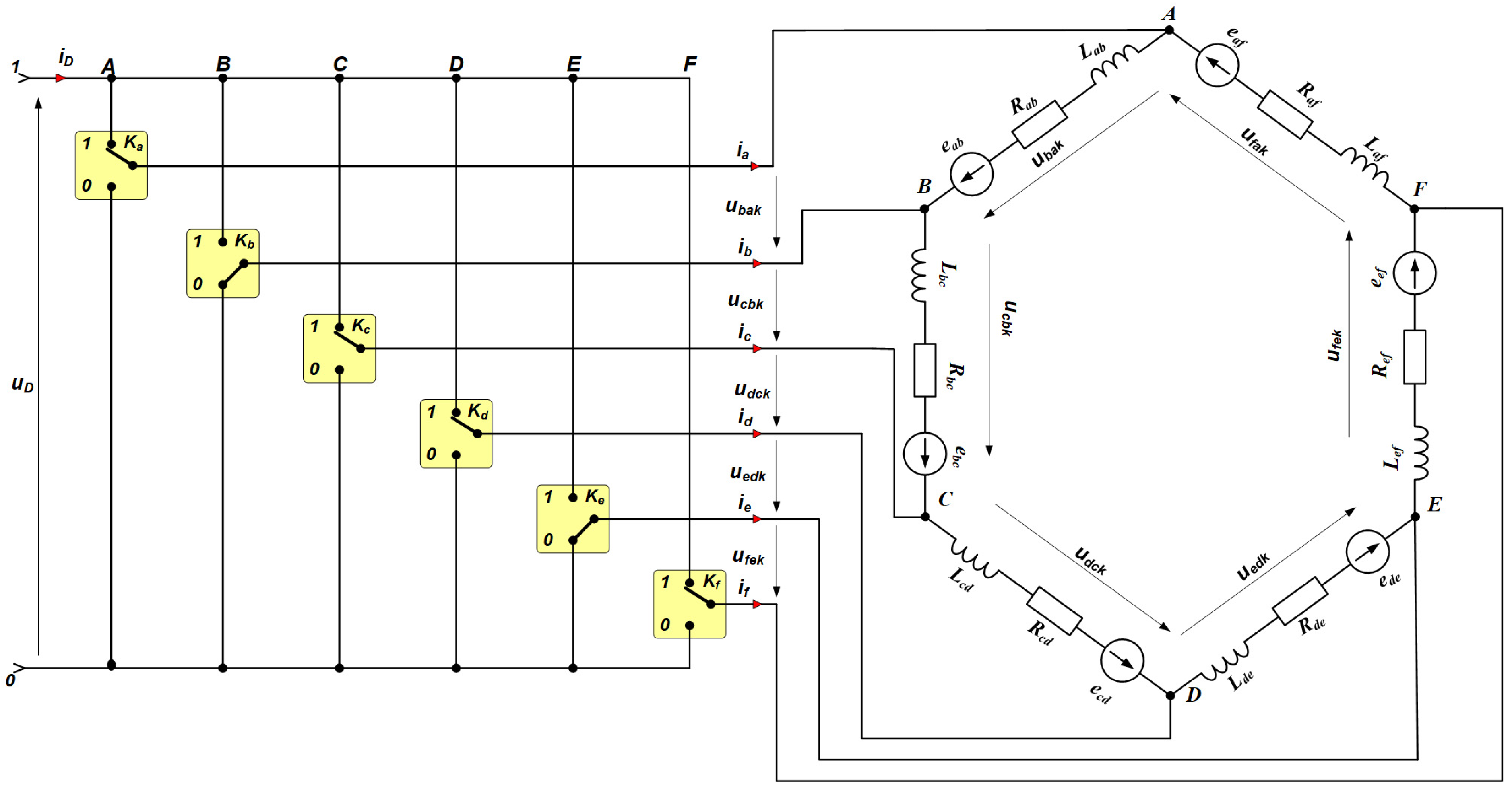
2.1. Model of Six-Phase Two-Level Inverter

Figure 1 depicts a simplified diagram of the six-phase two-level converter. The proposed model consists of six two-state switches denoted as Ka, Kb, Kc, Kd, Ke, Kf that are connected to the UD voltage source and associated with the corresponding phases. The voltage source’s positive pole is denoted as 1, whereas the negative is 0. Each switch has the ability to connect one source’s pole to the output of a particular phase, and hence the switching states are denoted by the 0 or 1 digit. The state of an inverter can be therefore expressed by the set of six digits including the switches’ states, which are denoted as a, b, c, d, e, f = 0, 1. That set can be represented by 64 variations, for instance 000000, 000001, …111111. A common method that is very useful is the assumption that such sets of digits form binary numbers, and hence a particular inverter’s state is determined by one binary number consisting of six digits. The most important issue is the precise consistency between the digits’ order and phases’ order. There is a possibility to express all 64 states of the inverter by decimals 0, 110, …6410 with the usage of the conversion of the binary numbers to the decimal (base-10) system. In this way, the 1610 (010000)2 state signifies that phases a, c, d, e are connected to the voltage source’s negative pole, whilst phase b to the positive. Such a method, with the exclusion of decimal numbers, can be utilized in the other notation systems.
The base-2 and base-10 number systems have been applied to describe two-level inverter states from the very beginning of the power electronics development. However, the principle of a precisely controlled “number–phase” relationship was not always maintained. The above discussion is cited here because the description concept presented can be applied to other converters. A way to describe multi-phase (n-phase) or even multi-level (n-level) converters may arise with further development of this concept.
In order to provide the reader with a cohesive and precise description of obtained experimental results, this section is divided into subsections. They include the interpretation of achieved results, as well as the drawn conclusions.

2.2. State Vectors of the Six-Phase Two-Level Inverter

According to the model in Figure 1, the six-phase two-level voltage source inverter (VSI) has 64 diverse switching states, denoted by decimal index k = 0, 1, …, 63, respectively. Particular k-states determine the six phase-to-phase voltages that appear at the output of the inverter. The six-phase VSI state vector is defined as a matrix row composed of six elements:
V k = [ U a b k   U b c k   U c d k   U d e k   U e f k   U f a k ]   k = 0 ,   1 ,   2 ,   ,   63
Assuming U a b k + U b c k + U c d k + U d e k + U e f k + U f a k = 0 , the state vector Vk s determined by a set of five Uxy phase-to-phase voltages under the condition that x and y denote the neighboring phases: xy and x, y = a, b, c, d, e, f.
The phase-to-phase voltage is formed by a difference between the particular phase outputs’ potentials. The switch Ka,b,c,d,e,f attaches the related phase output to one pole of the voltage source Ud. The state of the Ka,b,c,d,e,f is determined by the selected vector Vk.
The decimal vector index k can be reconverted to the binary number system and written as a binary number:
k = ( a k ,   b k ,   c k ,   d k ,   e k ,   f k ) 2  
where a k ,   b k ,   c k ,   d k ,   e k ,   f k = 0 ,   1 and k = 0, 1, 2, …, 63.
The phase output potentials related to the negative pole of the voltage source Ud are defined using the relevant binary symbol. Thus, the phase output polar voltages are
[ u a 0 k   = a k U D u b 0 k   = b k U D u c 0 k   = c k U D u d 0 k   = d k U D u e 0 k   = e k U D u f 0 k   = f k U D ]
It allows for the definition of a six-phase two-level VSI state vector using the binary symbols of the decimal index k. The transpose of the matrixVk llows for the presentation in one column of all six phase-to-phase voltages:
V k = [ u a b k   u b c k   u c d k   u d e k   u e f k   u f a k   ] = [ u a 0 k   u b 0 k   u b 0 k   u c 0 k   u c 0 k   u d 0 k   u d 0 k   u e 0 k   u e 0 k   u f 0 k   u f 0 k   u a 0 k   ] = U D [ ( a k b k ) 2 ( b k c k ) 2 ( c k d k ) 2 ( d k e k ) 2 ( e k f k ) 2 ( f k a k ) 2 ]
The symbols a k ,   b k ,   c k ,   d k ,   e k ,   f k may be equal only to 0 or 1, so any phase-to-phase voltage may assume one of these voltages: 0, +Ud, −Ud.
The inverter state vector Vk operates on physical quantities. Therefore, in order to calculate the load currents, there is no need to use a mathematical transform. A diagram of the six-phase two-level inverter with a load connected in a hexagon is shown in Figure 2. It assumes the symmetry of the load as well as the equality between each phase-to-phase load and two-terminal networks: <resistor R—inductance L—counter RMF>—connected in series. The inverter state is determined by the vector Vk, which means that the six corresponding phase-to-phase voltages are connected to the load. Figure 3 depicts the operation point in which phases a, c, d, f are connected to the pole 1 (+UD), whereas remaining phases are connected to the pole 0 (−UD). Therefore, the state vector is determined as V45(101101).
The adequate phase-to-phase voltages are given in (4). For any vector Vk switched on at a time equal to t = tn, the inverter model can be transformed to an equivalent circuit described by the set of six equations. Each equation can be expressed by
u x y k = R x y i x y ( t ) + L x y d i x y ( t ) d t + E x y ( t ) ,
where x and y denote the adjacent phases: xy and x, y = a, b, c, d, e, f. The voltage uxyk is defined based on (4) as
u x y k = [ u x 0 k u y 0 k ] = U D [ x k y k ]
Assuming that the EMFxy counter is constant in a time interval t < t n , t n + 1 > and equal to Exy respectively, it is possible to solve the equations and write expressions describing load currents (7). The symbol τ denotes the time constant of one load leg and I0xy—the current value in the time instant tn. The expressions (7) are valid in the definite time interval between the successive switching of the inverter states Vk(n) and Vk(n+1). The time interval is assumed to be exceptionally short in comparison with the time constant of the load circuit and the expected period of the counter electromotive force (EMF).
i x y k = [ u x y k E x y ] 1 e t τ R + I 0 x y e t τ   k = 0 ,   1 ,   2 ,   ,   63
where the time constant of the two-terminal network is τ = L x y R x y .
The expressions (6) and (7) define the dependence between phase-to-phase voltage and load current using the appropriate symbols of the vector index k binary expansion.

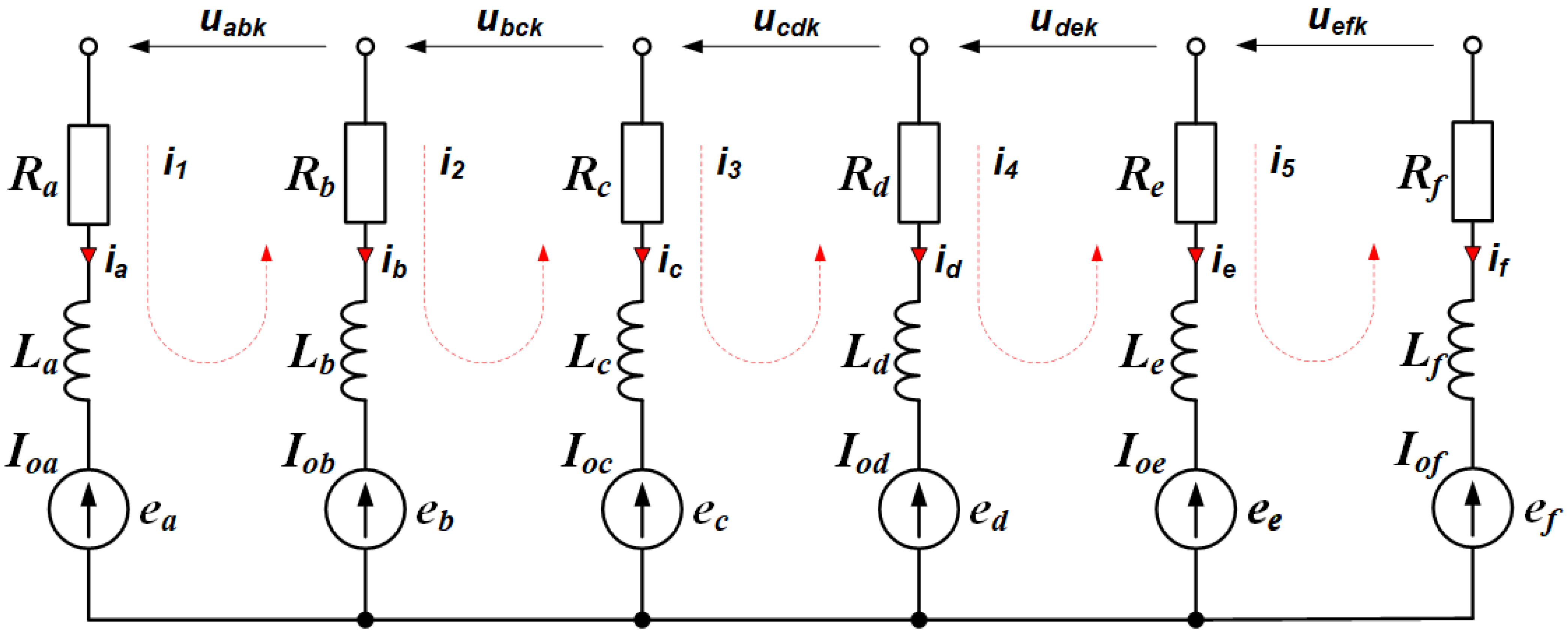
2.3. Star Connected Load of the Six-Phase Two-Level Inverter

The six-phase two-level inverter model with a star connected load is presented in Figure 3.
For any selected vector Vk in the time instant t = tn, the load-inverter model can be reduced to the equivalent five-closed-loop circuits shown in Figure 4.
Considering the time point t = tn when the state vector Vk is switched on, as well as assuming it is acting in a very short time interval t < t n , t n + 1 > , the following assumptions can be made:
u x y k = U x y k ,   e x = E x  
where x and y denote the adjacent phases: x y ,   x ,   y = a k ,   b k ,   c k ,   d k ,   e k ,   f k .
The phase-to-phase voltages are constant, and the phase counter EMFs are as well. In the considered system, the following dependences are obligatory:
e a + e b + e c + e d + e e + e f = 0 i a + i b + i c + i d + i e + i f = 0 I 0 a + I 0 b + I 0 c + I 0 d + I 0 e + I 0 f = 0
Assuming the phase load is fully symmetrical, the circuit’s mathematical model is described by the system of five equations:
{ U a b k ( t ) = R · i 1 ( t ) + L d i 1 ( t ) d t + E a E b + L d [ i 1 ( t ) i 2 ( t ) ] d t + R [ i 1 ( t ) i 2 ( t ) ] U b c k ( t ) = R [ i 2 ( t ) i 1 ( t ) ] + L d [ i 2 ( t ) i 1 ( t ) ] d t + E b E c + L d [ i 2 ( t ) i 3 ( t ) ] d t + R [ i 2 ( t ) i 3 ( t ) ] U c d k ( t ) = R [ i 3 ( t ) i 2 ( t ) ] + L d [ i 3 ( t ) i 2 ( t ) ] d t + E c E d + L d [ i 3 ( t ) i 4 ( t ) ] d t + R [ i 3 ( t ) i 4 ( t ) ] U d e k ( t ) = R [ i 4 ( t ) i 3 ( t ) ] + L d [ i 4 ( t ) i 3 ( t ) ] d t + E d E e + L d [ i 4 ( t ) i 5 ( t ) ] d t + R [ i 4 ( t ) i 5 ( t ) ] U e f k ( t ) = R [ i 5 ( t ) i 4 ( t ) ] + L d [ i 5 ( t ) i 4 ( t ) ] d t + E e E f + L d i 5 ( t ) d t + R · i 5 ( t ) }
The phase and loop currents relations are the following:
i a k ( t ) = i 1 ( t ) ,   i b k ( t ) = i 2 ( t ) i 1 ( t ) ,   i c k ( t ) = i 3 ( t ) i 2 ( t )
i d k ( t ) = i 4 ( t ) i 3 ( t ) ,   i e k ( t ) = i 5 ( t ) i 4 ( t ) ,   i f k ( t ) = i 5 ( t )
The relations between phase and phase-to-phase voltages remain, as follows (13):
U a = 5 6 U a b + 2 3 U b c + 1 2 U c d + 1 3 U d e + 1 6 U e f U b = 1 6 U a b + 2 3 U b c + 1 2 U c d + 1 3 U d e + 1 6 U e f U c = 1 6 U a b 1 3 U b c + 1 2 U c d + 1 3 U d e + 1 6 U e f U d = 1 6 U a b 1 3 U b c 1 2 U c d + 1 3 U d e + 1 6 U e f U e = 1 6 U a b 1 3 U b c 1 2 U c d 2 3 U d e + 1 6 U e f U f = 1 6 U a b 1 3 U b c 1 2 U c d 2 3 U d e 5 6 U e f
Two examples of this relation are presented below in Figure 5. They demonstrate the phase voltage vectors Ua, Uf as a sum of all phase-to-phase voltage vectors.
The phase voltages Uxk depend on selected vectors Vk. Knowledge of these voltages is indispensable if the system of equations is to be solved. In order to receive the final solution of the system (10), the Laplace transform has been used as the most convenient mathematical tool. Using this instrument, it was possible to solve the system and find the analytical expressions describing the phase voltage and current. The Laplace transform of successive phase currents is given as
I x k ( s ) = U x k E x L ( s + 1 τ ) + I 0 x s + 1 τ
while the inverse Laplace transform leads to the analytical expressions of phase currents. They are expressed by
i x k ( t ) = U x k E x R ( 1 e t τ ) + I 0 x e t τ  
where the index x denotes the successive phases x = a, b, c, d, e, f, and E x = E m a x sin ( ω t n + φ x )  Emax and φx are EMF parameters at the time instant t = tn.
The phase voltage Uxk depends on the selected vector and does not depend on the counter EMF.
In the considered wye load circuit, the phase voltage can be evaluated by the binary symbols of the decimal vector index k a k ,   b k ,   c k ,   d k ,   e k ,   f k as in the way presented in [35]. The phase voltages u a k ,   u b k ,   u c k ,   u d k ,   u e k ,   u f k of the two-level six-phase VSI are:
[ u a k   u b k   u c k   u d k   u e k   u f k   ] = U D 6 [ 5 a k b k c k d k e k f k 5 b k a k c k d k e k f k 5 c k a k b k d k e k f k 5 d k a k b k c k e k f k 5 e k a k b k c k d k f k 5 f k a k b k c k d k e k ]
The considered six-phase VSI has 64 state vectors determining all possible voltage states of the inverter. Each vector represents its own phase connection to the supply voltage UD. A few examples of potential circuits are presented in Figure 5.
Figure 6 presents selected load configurations. The arrangement presented in 6a conforms to the vector V56(111000), which means that three phases (a, b, c) are connected to the pole 1 of the voltage source (+UD), while the remaining phases are connected to the pole 0. Assuming all phase impedances Z equal the supply voltage, UD is divided into two values, 0.5UD and −0.5UD, referenced to the neutral point N. This result determines the phase voltages ua56, ub56, uc56 equal to +0.5UD and ud56, ue56, uf56 equal to −0.5UD, respectively. The other few proposed load configurations are presented in Figure 6b–d. They present three diversified states: V44(101100), V21(010101), V8(001000), respectively. For the two first vectors, the UD division is the same as in case 6a, but different phases have positive or negative phase voltages, while the case 6d presents the situation when only one phase c is connected to the pole 1 (+UD). Thus, the result in the phase c voltage equals +0.8UD while the remaining phases, connected to the pole 0, are supplied by voltage −0.2UD. Among 64 vectors, there are six thinkable combinations of load configuration when only one phase is connected to the pole 1 (+UD) and the next six when the one phase is connected to the pole 0 ( U D ) because mathematically ( 6 1 ) = ( 6 5 ) = 6 . All the remaining combinations ( 6 2 ) = ( 6 4 ) = 15 ,   ( 6 3 ) = 20 ,   ( 6 6 ) = ( 6 0 ) = 1 are implicated in the consequent 52 states. The last two states demonstrate the situation when all phase-to-phase voltages uxy(0 or 63) are equal to zero, so they do not influence the phase currents. They are usually called “zero vectors”.

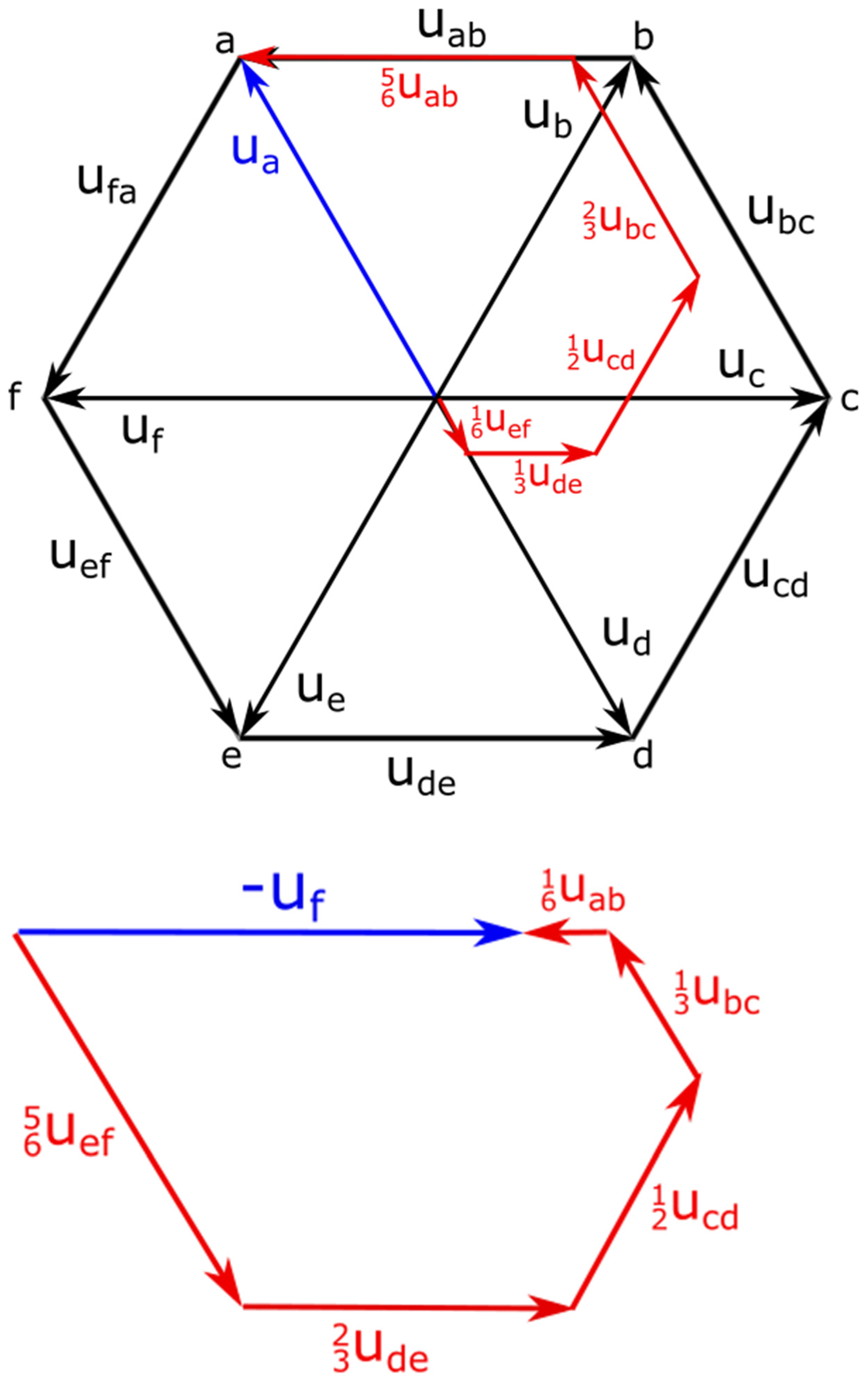
2.4. Polar Voltage Space Vectors of the Six-Phase Two-Level Voltage Source Inverter

The polar voltage space vector of the two-level six-phase VSI is determined analogically to the way presented in the previous sections. The definition was established as
V - k = 5 6 ( u a 0 k + q u b 0 k + q 2 u c 0 k + q 3 u d 0 k + q 4 u e 0 k + q 5 u f 0 k )
where q = e j 2 π / 6 = cos 60 ° + j s i n 60 ° = 1 2 + j 3 2 .
V - k = 5 6 U D ( a k + b k e j π 3 + c k e j 2 π 3 + d k e j π + e k e j 4 π 3 + e k e j 5 π 3 )
Equation (18) expresses the space vector which is defined in symbols of the index k binary expansion. The index k is a decimal number discriminating the state vector k = ( a k b k c k d k e k f k ) 2 , where { a k , b k , c k , d k , e k , f k } = { 0 , 1 } .
Applying Euler’s formula and introducing interdependences among the angles, as well as symbols a k ,   b k , c k , d k , e k , f k , the space vector is given as follows:
V - k = 5 6 U D [ a k d k + 1 2 ( b k c k e k + f k ) + j 3 2 ( b k + c k e k f k ) ]
After the transformation, the space vector is a complex number which may be represented by the modulus Mk and the argument φk. However, in the case of the six-phase inverter, the situation is more demanding in comparison with three-phase inverters due to a greater number of variables. The expression allowing calculation of the space vector modulus is the following:
M k = K γ 0 + γ 1 + γ 2 + γ 3 + γ 4 + γ 5
where K is a constant of proportionality and a coefficient which depends on UD. The coefficients γ 0 ,   γ 1 , γ 2 , γ 3 , γ 4 , γ 5 are as follows:
γ 0 = a k 2 + b k 2 + c k 2 + d k 2 + e k 2 + f k 2 γ 1 = a k ( b k c k 2 d k e k + f k ) γ 2 = b k ( c k d k 2 e k f k ) γ 3 = c k ( d k e k 2 f k ) γ 4 = d k ( e k f k ) γ 5 = e k f k
If the constant K equals 5 6 U D , then, according to (20), the modulus Mk may reach four diverse values: 0 ,   5 6 U D ,   5 3 U D ,   5 6 3 U D . The value of the constant K may differ depending on the assumed canon.
The vectorial angle φk is determined using trigonometrical functions. In some cases, it might be necessary to use both functions, arctg and arcsin, due to diverse periodicity of sine and tangent. Then, the angle of the vector is determined if ϕ k ( a r c s i n ) = ϕ k ( a r c t g ) . Formula (22) allows for the calculation of the ϕ k value:
ϕ k = arcsin   3 ( b k + c k e k f k ) 2 M k ,   ϕ k = a r c t g 3 ( b k + c k e k f k ) 2 ( a k d k ) + b k c k e k + f k
The denominator of the expressions (22) cannot equal zero. Thus, the results of ϕ k are indeterminate for a k = b k = c k = d k = e k = 0 or a k = b k = c k = d k = e k = 1 . The corresponding two vectors V0(000000) and V63(111111) are habitually named zero vectors because they do not have any impact on the phase currents. The parameters moduli Mk and shift angles φk of all 62 active vectors are collected in Table 1. The constant K of the vectors used in the consideration was assumed K = 5 6 U D .
Figure 7 and Figure 8 present the polar voltage space vectors of the six-phase inverter. They are presented on the complex plane (α − jβ) where α denotes the real axis and β—the imaginary one. The diagram presents their position. Each marked point denotes at least one sense of a vector. The smallest points denote one vector, while the bigger ones—two, six, and ten. The next further down diagram indicates the binary expansions of all the numbers defining the relevant vectors. According to the assumption K = 5 6 U D , the vector moduli reach only four values: 0 ,   1 , 3 , 2 .
Apart from two zero vectors in the middle of 62 vectors, there are four groups of active vectors: six vectors with moduli 2, twelve with moduli 3 , thirty-six with 1, and also eight active vectors which formally have zero-dimensional moduli and indeterminate angles. Among these eight vectors, two of them, V21 as well as V42, can be considered as representing two three-phase voltage systems (Table 2). The first one could be determined by three voltages: Vb, Vd, Vf and the other, by voltages: Va, Vc, Ve.
Another possibility to reach two three-phase voltage systems is accessible using the next six active vectors which formally have zero-dimensional moduli, that is: V9, V18, V27, V36, V45, V54. These ones present the symmetry ak, bk, ck = dk, ek, fk in the binary expansion of the vector number. The vectors are collected below in different sequences. The sequences ak, bk, ck and dk, ek, fk are suitable to control the three-phase system. Thus, following the order indicated in Table 2, it is possible to control two twin three-phase AC drives. Formally, the vectors’ angle φk is indeterminate, but in Table 3 the angle φk was assumed in theory for application in standard α-β transform and used routinely in three-phase systems to control AC drives.
The control process of twin AC drives consists of switching of the successive vectors starting from vector V36. The sequence of vectors is evident according to the angle φk. The pairs of vectors V 36 V 54 ,   V 54 V 18 ,   V 18 V 27 ,   V 27 V 9 ,   V 9 V 45 ,   V 45 V 36 relate to the consecutive sectors of the stationary coordinate system on the complex plane α-jβ.

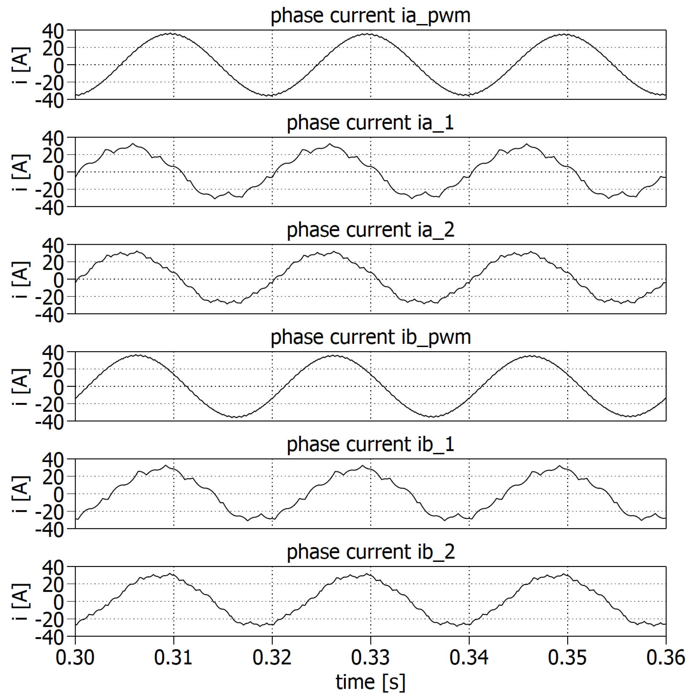
3. Simulation Experiment

The described methodology of using polar voltage space vectors intended to control six-phase VSIs was tested during simulation tests. The tests included two scenarios. In the first scenario, the computed PWM modulation vectors at RL load were performed, while in the other scenario, the applied load simulated an induction motor. For illustration purposes, in the course of the simulation tests, the applied control method consisted of simple concatenation of the consecutive vectors. Each next vector activated switching in only one phase of the inverter.
Figure 8 shows the vector map for the first control strategy in a graphical form, while Figure 9 presents the modified sequence of the calculated vectors, which consisted of repeating the sequence in each sector. This treatment produced interesting results. It should also be noted that the graphical representations of the vectors in each sector shown in Figure 8 and Figure 9 were achieved by mirroring. The vectors’ sequences shown in Figure 9 and Figure 10 were selected according to the above mentioned rule of one switching in one phase.
Figure 11 shows the diagram of the simulation model, in which the control tests were carried out. The PWM method and two control strategies presented in Figure 9 and Figure 10 were compared.
Figure 12 shows the waveforms of the control signals corresponding to the individual control systems. The figures show the signals for phases a and b.
Figure 13 shows the phase-to-phase voltage waveforms: Uba and Ucb.
Figure 14 shows the phase currents ia and ib obtained for different control strategies.
Table 3 presents a summary of the most important parameters obtained during the simulation tests. The PWM method was compared with the vector control strategy. The mark 1 denotes a single sequence of vectors and the mark 2—a sequence of vectors repeated in every sector. The load parameter RL was assumed as R = 2 Ω and L = 40 mH, which means the time constant was τ = 20 ms. Table 4 presents the RMS and THD current values for different frequencies in the range 40–60 Hz.
The control strategy number 1 has been chosen so that the switching of the keys in a given clock takes place only once. The control strategy 2 is a double repetition in a cycle of the control strategy 1. Using such a simple control method, very good results have been obtained for the content of higher harmonics, which can be seen from the THD values. At the same time, the adopted control also allows for maintaining a high rms value of the currents. Subsequent repetition of the adopted vector sequence would lead to results comparable to PWM control. However, the main advantage of the control method described in the experiment over PWM is that it requires a much smaller amount of switching.
In the referenced works [36,37], the described control algorithm was used for inverters with an odd number of phases. Three-phase [37] and five-phase [36] inverters were considered. On the other hand, Table 5 shows the results of simulation tests for a five-phase inverter, which are to be used to compare both cases. These tests were carried out for the same scenario, i.e., the control of PWM modulation and vector control for single and double repetitions of vector sequences were compared.
Summarizing the results presented in Table 5, it can be concluded that they are generally similar. In the case of a five-phase inverter, a higher RMS value can be observed, but its performance has deteriorated due to an increase in the current THD value. One can risk a statement that an increase in the number of inverter phases reduces the THD value. This can be explained by the fact that with a greater number of phases, their interaction affects the reduction of higher harmonics.

4. Conclusions

The aim of the paper was to prove that state and polar voltage space vectors are a useful mathematical tool in the analysis and control of a six-phase inverter. Typically, the inverter model can be described with the use of three mathematical tools: analytic expressions, the voltage state, and space vectors. The analytic formulas determine the inverter phase current and voltage, whereas the state voltage vectors define phase voltage distribution in all the states of the inverter. Furthermore, polar voltage space vectors are a very valuable and well recognized instrument in inverters’ control. They constitute a simple and basic tool that can be applied in the space vector method, which is the most widespread contemporary control method in AC drives. The whole control process is restricted to the simplest concatenation of successive vectors. This way of control permits to limit to a minimum the number of switching and zero vectors used, as well as avoiding problems resulting in parity of phases. This control method seems to be especially suitable for inverters working in the range of relatively higher frequencies 40–60 Hz, e.g., inverters interfacing a six-phase smart grid and a solar power plant.
The described simulation examples of the inverter vector control based on the polar voltage space vectors proved that the proposed solution might be indeed suitable in designing inverter control algorithms. The presented space vector method assures a significantly lower number of inverter switching in comparison with the PWM. It also results in higher efficiency of the inverter.
Both the notation and computational method described in this paper have been used in previous works related to multi-phase inverters. However, only the inverters with an odd number of phases, i.e., three and five, have been considered there [36,37]. This paper presents the synthesis and analysis for an inverter with an even number of phases. Although it seemed there should be no problematic issues at first, an even number of phases greatly complicated the whole computational process since the choice of vectors in such a case was further limited by the symmetry of phases, which was not present in the case of an odd number of phases. This is also a justification for why various methods have been used for six-phase inverters to avoid phase symmetry. Among them, there are shifting the initial phase by 30 degrees or analyzing the six-phase inverter as two three-phase inverters. Another encountered problem was that even though it was possible to find vector sequences that were optimal in terms of the amount of switching, they were not implementable in the inverter due to the asymmetry of the voltage and current waveforms that were generated by the inverter. Based on the analysis in this paper as well as previous papers on multiphase inverters, it is easier to obtain vector sequences that meet control expectations for inverters with an odd number of phases than for inverters with an even number of phases.
The simulation experiment described in this paper shows that the assumed vector strategy allows for the obtaining of a favorable value of current THD with the simultaneous preservation of the currents’ rms values in comparison to PWM modulation. The experiment also presents that repetition of the proposed vector sequence influences the further reduction of the harmonic content and increase in the rms value of the currents.

Author Contributions

Conceptualization, J.I.; methodology, J.I.; formal analysis, J.I. and A.M.; investigation, J.I. and A.M.; writing—original draft preparation, J.I., A.M. and A.B.; supervision, J.I. All authors have read and agreed to the published version of the manuscript.

Funding

This project is financially supported under the framework of a program of the Ministry of Science and Higher Education (Poland) as “Regional Excellence Initiative” in the years 2019–2022, project number 006/RID/2018/19, amount of funding 11 870 000 PLN.

Institutional Review Board Statement

Not applicable.

Informed Consent Statement

Not applicable.

Data Availability Statement

Not applicable.

Conflicts of Interest

The authors declare no conflict of interest.

References

  1. Listwan, J.; Pieńkowski, K. Field-Oriented Control of Five-Phase Induction Motor with Open-End Stator Winding. Arch. Electr. Eng. 2016, 65, 395–410. [Google Scholar]
  2. Levi, E.; Bojoi, R.; Profumo, F.; Toliyat, H.A.; Williamson, S. Multi-phase induction motor drives—A technology status review. IET Electr. Power Applications 2007, 1, 489–516. [Google Scholar] [CrossRef] [Green Version]
  3. Levi, E. Multi-phase electric machines for variable-speed applications. IEEE Transactions Ind. Electron. 2008, 55, 1893–1909. [Google Scholar] [CrossRef]
  4. Chavan, G.; Sridhar, S. Speed Control of Dual Induction Motor Using Five Leg Inverter. E3S Web Conf. 2020, 184, 01065. [Google Scholar] [CrossRef]
  5. Okayasu, M.; Sakai, K. Novel integrated motor design that supports phase and pole changes using multi-phase or single phase inverters. In Proceedings of the 2016 18th European Conference on Power Electronics and Applications (EPE’16 ECCE Europe), Karlsruhe, Germany, 5–9 September 2016; p. 135. [Google Scholar]
  6. Vasile, I.; Tudor, E.; Popescu, M.; Dumitru, C.; Popovici, L.; Sburlan, I.C. Electric Drives with Multi-phase Motors as a Better Solution for Traction Systems. In Proceedings of the 2019 11th International Symposium on Advanced Topics in Electrical Engineering (ATEE), Bucharest, Romania, 28–30 March 2019. [Google Scholar]
  7. Jakubiec, B. Multi-phase Permanent Magnet Synchronous Motor Drive for Electric Vehicle. Przegląd Elektrotechniczny 2015, 91, 125–128. [Google Scholar]
  8. Meinguet, F.; Nguyen, N.-K.; Sandulescu, P.; Kestelyn, X.; Semail, E. Fault-Tolerant Operation of an Open-End Winding Five-Phase PMSM Drive with Inverter. In Proceedings of the IECON 39th Annual Conference of the IEEE Industrial Electronics Society, Singapore, 18–21 October 2013. [Google Scholar]
  9. Omata, R.; Oka, K.; Furuya, A.; Matsumoto, S.; Nozawa, Y.; Matsuse, K. An Improved Performance of Five-Leg Inverter in Two Induction Motor Drives. In Proceedings of the 2006 CES/IEEE 5th International Power Electronics and Motion Control Conference, Shanghai, China, 14–16 August 2006. [Google Scholar]
  10. Ruba, M.; Surdu, F.; Szabo, L. Study of a Nine-Phase Fault Tolerant Permanent Magnet Starter-Alternator. J. Comput. Sci. Control Syst. 2011, 4, 149–154. [Google Scholar]
  11. Farsadi, M.; Kalashani, M.B. A novel hybrid multi-phase multilevel inverter topology. In Proceedings of the 10th International Conference on Electrical and Electronics Engineering (ELECO), Bursa, Turkey, 30 November–2 December 2017; pp. 305–308. [Google Scholar]
  12. Muqorobin, A.; Dahono, P.A.; Purwadi, A. Optimum phase number for multi-phase PWM inverters. In Proceedings of the 2017 4th International Conference on Electrical Engineering, Computer Science and Informatics (EECSI), Yogyakarta, Indonesia, 19–21 September 2017; pp. 1–6. [Google Scholar]
  13. Vitale, G.P.; Pipitone, E. A Six Legs Buck-boost Interleaved Converter for KERS Application. In Proceedings of the The International Conference ICREPQ’20, Granada, Spain, 8–10 April 2020. [Google Scholar]
  14. Furkan, A.; Yakup, T.; Enes, U.; Bulent, V.; Ismail, A. A bidirectional non-isolated multi-input DC–DC converter for hybrid energy storage systems in electric vehicles. IEEE Trans. Vehic. Technol. 2015, 65, 7944–7955. [Google Scholar]
  15. Padmanaban, S.; Hontz, M.R.; Khanna, R.; Wheeler, P.W.; Blaabjerg, F.; Ojo, J.O. Isolated/non-isolated quad-inverter configuration for multilevel symmetrical/asymmetrical dual six-phase star-winding converter. In Proceedings of the 2016 IEEE 25th International Symposium on Industrial Electronics (ISIE), Santa Clara, CA, USA, 8–10 June 2016; pp. 498–503. [Google Scholar]
  16. Moinoddin, S.; Iqbal, A.; Abu-Rub, H.; Khan, M.R.; Ahmed, S.M. Three-Phase to Seven-Phase Power Converting Transformer. IEEE Trans. Energy Convers. 2012, 27, 3. [Google Scholar]
  17. Abdel-Rahim, O.; Funato, H.; Abu-Rub, H.; Ellabban, O. Multi-phase Wind Energy Generation with Direct Matrix Converter. In Proceedings of the 2014 IEEE International Conference on Industrial Technology (ICIT), Busan, Korea, 26 February–1 March 2014. [Google Scholar]
  18. Koptjaew, E.; Popkov, E. AC-multi-phase Adjustable Electric Drive with Two-channel Conversion. In Proceedings of the International Conference on Industrial Engineering Applications and Manufacturing, ICIEAM, Pilsen, Czech Republic, 23–26 July 2019. [Google Scholar]
  19. Gao, Z.; Lu, Q. A hybrid cascaded multilevel converter based on three-level cells for battery energy management applied in electric vehicles. IEEE Trans. Power Electron. 2018, 34, 7326–7349. [Google Scholar] [CrossRef]
  20. Malinowski, M.; Gopakumar, K.; Rodriguez, J.; Perez, M.A. A Survey on Cascaded Multilevel Inverters. IEEE Trans. Ind. Electron. 2010, 57, 2197–2206. [Google Scholar] [CrossRef]
  21. Sleszynski, W.; Cichowski, A.; Mysiak, P. Suppression of supply current harmonics of 18-pulse diode rectifier by series active power filter with lc coupling. Energies 2020, 13, 6060. [Google Scholar] [CrossRef]
  22. Hui, P.; Wang, J.; Shen, W.; Shi, D.; Huang, Y. Controllable regenerative braking process for hybrid battery–ultracapacitor electric drive systems. IET Power Electron. 2018, 11, 2507–2514. [Google Scholar]
  23. Łebkowski, A.; Koznowski, W. Analysis of the use of electric and hybrid drives on swath ships. Energies 2020, 13, 6486. [Google Scholar] [CrossRef]
  24. Rybczak, M.; Rak, A. Prototyping and simulation environment of ship motion control system. TransNav 2020, 14, 367–374. [Google Scholar]
  25. Łebkowski, A. Analysis of the Use of Electric Drive Systems for Crew Transfer Vessels Servicing Offshore Wind Farms. Energies 2020, 13, 1466. [Google Scholar] [CrossRef] [Green Version]
  26. Nguyen, N.; Oruganti, S.K.; Na, K.; Bien, F. An adaptive backward control battery equalization system for serially connected lithium-ion battery packs. IEEE Trans. Veh. Technol. 2014, 63, 3651–3660. [Google Scholar] [CrossRef]
  27. Listwan, J. Application of Super-Twisting Sliding Mode Controllers in Direct Field-Oriented Control System of Six-Phase Induction Motor: Experimental Studies. Power Electron. Drives 2018, 3, 23–34. [Google Scholar] [CrossRef] [Green Version]
  28. Liu, Z.; Zheng, Z.; Sudhoff, S.D.; Gu, C.; Li, Y. Reduction of common-mode voltage in multi-phase two-level inverters using SPWM with phase shifted carriers. IEEE Trans. Power Electron. 2016, 31, 6631–6645. [Google Scholar] [CrossRef]
  29. Nie, Z.; Preindl, M.; Schofield, N. SVM strategies for multi-phase voltage source inverters. In Proceedings of the 8th IET International Conference on Power Electronics, Machines and Drives (PEMD 2016), Glasgow, UK, 19–21 April 2016; pp. 1–6. [Google Scholar]
  30. Ippisch, M.; Gerling, D. Analytic Calculation of Space Vector Modulation Harmonic Content for Multi-phase Inverters with Single Frequency Output. In Proceedings of the IECON 2019—45th Annual Conference of the IEEE Industrial Electronics Society, Lisbon, Portugal, 14–17 October 2019; pp. 6187–6193. [Google Scholar]
  31. Karugaba, S.; Ojo, O. A carrier-based PWM modulation technique for balanced and unbalanced reference voltages in multi-phase voltage-source inverters. IEEE Trans. Ind. Appl. 2012, 48, 2102–2109. [Google Scholar] [CrossRef]
  32. Wang, Y.; Li, Y. Generalized Theory of Phase-Shifted Carrier PWM for Cascaded H-Bridge Converters and Modular Multilevel Converters. IEEE J. Emerg. Sel. Top. Power Electron. 2016, 4, 589–605. [Google Scholar] [CrossRef]
  33. Vafakhah, B.; Salmon, J.; Knight, A.M. A New Space-Vector PWM with Optimal Switching Selection for Multilevel Coupled Inductor Inverters. IEEE Trans. Ind. Electron. 2010, 57, 2354–2364. [Google Scholar] [CrossRef]
  34. Dujic, D.; Jones, M.; Levi, E. Generalized space vector PWM for sinusoidal output voltage generation with multi-phase voltage source inverters. Int. J. Ind. Electron. And Drives 2009, 1, 1–13. [Google Scholar] [CrossRef]
  35. Grandi, G.; Serra, G.; Tani, A. Space Vector Modulation of a Six Phase VSI based on three-phase decomposition. In Proceedings of the 2008 International Symposium on Power Electronics, Electrical Drives, Automation and Motion, Sorrento, Italy, 11–13 June 2008; pp. 674–679. [Google Scholar]
  36. Iwaszkiewicz, J.; Muc, A. State and Space Vectors of the 5-Phase 2-Level VSI. Energies 2020, 13, 4385. [Google Scholar] [CrossRef]
  37. Iwaszkiewicz, J.; Wolski, L. State and Space Vectors—Complementary Description of the 2-level VSI. In Proceedings of the International Conference on Renewable Energies and Power Quality (ICREPQ’14), Cordoba, Spain, 8–10 April 2014. [Google Scholar]
Figure 1. Simplified diagram of the six-phase two-level inverter with six switches.
Energies 15 02763 g001
Figure 2. The diagram of the six-phase two-level inverter with the hexagonal connected load according to the state vector V45(101101).
Energies 15 02763 g002
Figure 3. The model of the six-phase two-level inverter with the star connected load.
Energies 15 02763 g003
Figure 4. The model circuit of the six-phase two-level inverter with the star connected load.
Energies 15 02763 g004
Figure 5. The dependencies between voltage vectors Ua, Uf and phase-to-phase voltage vectors.
Energies 15 02763 g005
Figure 6. A few circuit examples of the star connected load: (a) topology of load for vector 111000; (b) topology for vector 101100; (c) topology for vector 010101; (d) topology for vector 001000.
Energies 15 02763 g006
Figure 7. The polar voltage space vectors of the two-level six-phase VSI.
Energies 15 02763 g007
Figure 8. The polar voltage space vectors of the two-level six-phase VSI and their binary expansions.
Energies 15 02763 g008
Figure 9. The polar voltage space vectors of the two-level six-phase VSI and their binary expansions.
Energies 15 02763 g009
Figure 10. The vector map for the other control strategy.
Energies 15 02763 g010
Figure 11. The schematic diagram of a six-phase VSI used to test the described system of the vectors.
Energies 15 02763 g011
Figure 12. The comparison of the control signal waveforms for various control strategies: a, b—phases; pwm—PWM modulation; 1—a single sequence of vectors; 2—a sequence of vectors repeated in every sector.
Energies 15 02763 g012
Figure 13. The comparison of the phase-to-phase voltage waveforms for various control strategies: pwm—PWM method; 1—a single sequence of vectors; 2—a sequence of vectors repeated in every sector.
Energies 15 02763 g013
Figure 14. The comparison of the phase current waveforms for different control strategies: a, b—phases; pwm—PWM method; 1—a single sequence of vectors; 2—a sequence of vectors repeated in every sector.
Energies 15 02763 g014
Table 1. The vectors’ parameters of the two-level six-phase inverter.
VkabcdefMkφkVkabcdefMkφk
V00000000*V3210000010
V10000011300V33100001 3 330
V20000101240V341000101300
V3000011 3 270V351000112300
V40001001180V361001000*
V50001011240V371001011300
V6000110 3 210V381001101240
V70001112240V39100111 3 270
V80010001120V40101000160
V90010010*V4110100110
V100010101180V421010100*
V110010111240V431010111300
V12001100 3 150V441011001120
V130011011180V451011010*
V140011102180V461011101180
V15001111 3 210V471011111240
V16010000160V48110000 3 30
V1701000110V4911000120
V180100100*V5011001010
V190100111300V51110011 3 330
V200101001120V52110100160
V210101010*V5311010110
V220101101180V541101100*
V230101111240V551101111300
V24011000 3 90V56111000260
V25011001160V57111001 3 30
V260110101120V58111010160
V270110110*V5911101110
V280111002120V60111100 3 90
V290111011120V61111101160
V30011110 3 150V621111101120
V310111111180V631111110*
* The sign denotes the vector angle is indeterminate.
Table 2. The two vectors representing the three-phase voltage system.
Vkabcdef
V21010101
V42101010
Table 3. The active vectors guaranteeing the symmetry ak, bk, ck = dk, ek, fk.
Three-Phase
AC Drive
Three-Phase
AC Drive
Vkabcdefφk
V361001000
V5411011060°
V18010010120°
V27011011180°
V9001001240°
V45101101300°
Table 4. The vectors’ parameters of the six-phase VSI inverter.
LoadR = 2 Ω, L = 40 mH
Control
Strategy:
F4045505560
PWMRMS23.924.324.023.522.8
THDI1.41.31.31.41.5
1RMS23.823.021.920.919.8
THDI9.69.79.69.69.5
2RMS24.123.222.221.019.9
THDI5.55.55.45.45.4
Table 5. The vectors’ parameters of the five-phase VSI inverter.
LoadR = 2 Ω, L = 40 mH
Control
Strategy:
F4045505560
PWMRMS27.726.725.524.323.1
THDI2.12.32.62.83.1
1RMS28.826.723.321.420.7
THDI11.511.511.611.711.8
2RMS29.226.624.323.121.9
THDI7.47.47.57.57.4
Publisher’s Note: MDPI stays neutral with regard to jurisdictional claims in published maps and institutional affiliations.

