1. Introduction
In mountainous or hilly regions wind turbines are sited along the crest of hills, ridgelines, or plateaus to take advantage of terrain-enhanced flows. Wind speeds can be enhanced by these terrain features through the compression of air as it is forced up and along the windward terrain slope towards a pressure minimum that develops at the top of a hill, such that the flow is no longer in logarithmic equilibrium under neutral stability and a maximum wind speed (Umax) or wind jet develops relatively close to the surface (e.g., [
1,
2]). This phenomenon is called a “hill-speed up” effect. It is represented by the fraction of change in the wind speed found on top of the hill to the undisturbed velocity found at an equivalent height at some distance upwind. Early experimental work suggested that the magnitude of the speed-up is proportional to the upwind slope of the hill [
3,
4] in agreement with the linearized theory of [
5]. Following evidence presented in [
6], a maximum hill speed-up should occur relatively close to the ground (at heights between 10–30 m) and within the layer of the atmosphere that the authors define as the inner flow region. At these heights, the flow field is in equilibrium with the surface and flow acceleration and the pressure gradient forces are all important. Atmospheric stability acts to not only intensify this hill speed-up effect, but also alter the height at which the wind maximum is found [
7].
Attempts to study and quantify the hill-speed up effect have been done using both traditional meteorological masts (e.g., [
7,
8,
9]) and more recently, with high-resolution, remote-sensing laser detection and ranging (lidar) instrumentation (e.g., [
10,
11,
12]). Study sites range from an isolated, single hill, to a coastal escarpment, to a multi-megawatt wind farm sited in hilly terrain. Attempts to forecast power generation at the latter site showed the difficulties in using machine learning techniques trained on lidar inflow data in complex terrain [
13]. That study showed that that rotor-disk wind speed above the hills was at times significantly higher than predicted based on the measured upwind profile. This suggested a strong hill-speed-up effect encountered by the 55 m tall turbines.
Since those data were collected in 2013, the Northern California Altamont Pass Wind Resource Area (APWRA) has been largely re-powered with turbines of larger rated capacities (2021 APWRA average = 1.7 MW) and higher hub-heights (2021 APWRA median = 80 m) than the 55 m tall, 1 MW turbines studied by [
10,
13]. Likewise, this trend in deploying taller, larger turbines is widespread throughout the United States. Larger hub-heights (U.S. 2020 mean = 90.1 m), rotor-disk lengths (mean = 124.8 m) and rated capacities (mean = 2.75 MW) have led to optimizations in onshore wind project cost and performance in many parts of the country, particularly in the flat Central U.S. [
14]. U.S. wind permitting data suggest that even taller turbines will be deployed onshore. Among proposed projects in the permitting processes, the average blade tip height of new turbines now reaches more than 200 m into the atmosphere. The drive for taller turbines is partially driven by the fact that wind speed typically increases with height at most locations, such that building higher into the atmosphere should tap into a greater wind resource. However, the validity of this assumption is questionable under certain wind flow environments. These include the presence of low-level jets [
15], large-scale, mountain-induced buoyancy waves [
16], variable atmospheric stability regimes [
17,
18,
19], and flow in areas of localized complex terrain [
20]. Moreover, changes in shear, veer, and turbulence associated with these flows add a secondary level of turbine-atmosphere and wind farm-atmosphere feedback complexity [
21].
In order to isolate one of these effects on the turbine wind resource, we examine here the hill-speed up phenomenon, and question whether building taller turbines in some areas of complex terrain does in fact typically increase the available wind resource. To examine this question, we present vertical profiles of wind speed and direction above two hills on parallel ridgelines (devoid of wind turbines) taken during an experiment called the Hill Flow Study, or HilFlowS [
22]. Comparison of the wind profiles by hill height, slope (as a function of predominant wind direction), and time of day are shown for the area’s peak power season. The observations also provide wind resource data for the APWRA to compare to the more classical logarithm wind profiles found over flatter terrain. Implications on the available wind resource from selecting new wind turbine models during regional re-powering are discussed in the context of how rotor-disk length and hub-height determine rotor-disk shear and the rotor-disk equivalent wind speed in hilly terrain. While of course, a smaller turbine with a smaller rated capability will generate less power no matter the difference in the wind resource (as long as the winds are between cut-in and cut-out), so we instead focus on comparing turbine models of roughly equal rated capabilities with different hub-heights and rotor-diameters.
Motivation for this new study was provided by earlier wind profile observations taken at Site 300 [
23] and the APWRA wind farm [
10], as well as observations taken by the U.S. Department of Energy (DOE)’s Second Wind Forecasting Improvement Project (WFIP2). WFIP2 was an intensive 18-month long field campaign in the Oregon-Washington Columbia Gorge and Columbia Basin Region designed to take a robust set of observations of wind flow in the atmospheric boundary layer for improving wind forecasting models in complex terrain [
24,
25,
26,
27]. HilFlowS was designed to provide a second set of wind observations over complex terrain in a different part of the U.S. to evaluate WFIP2’s physics and grid resolution improvements to the National Oceanic and Atmospheric Administration’s (NOAA) High-Resolution Rapid Refresh (HRRR) model, HRRRv4. Ongoing efforts are being made to test these improvements made in HRRRv4, including reducing the grid interval from 3 km to 750 m, for the HilFlowS domain. HilFlowS wind observations are available to the public on the DOE Atmosphere to Electrons (A2E) data portal (
https://a2e.energy.gov/projects/wfip2.hilflows, accessed on 30 March 2022).
2. Area Description and Wind Climatology
HilFlowS was conducted in the summer of 2019 at Lawrence Livermore National Laboratory’s Experimental Testing Site, called Site 300, which is 20 km east of the town of Livermore, California and approximately 85 km from the Pacific Ocean. The terrain is moderately complex and includes a part of the Diablo Range, a subsection of the California Coast Range mountains. Within 25 km of Site 300 major peaks range in elevation from 800 to 1100 m a.s.l. in the more complex south and southwest directions. The highest peaks to the west are 550–650 m a.s.l. Less complex terrain is found to the east and north where the terrain gently downslopes into the Central Valley and Delta Region. Ridgelines run roughly northwesterly to southeasterly in this part of the Diablo Range making them perpendicular to the predominant summertime, southwesterly (onshore) wind direction. Site 300 is covered by a maximum 1 m tall, seasonal grassland with very low surface roughness, especially during the summer months when the annual grasses have reached senescence. Upwind vegetation and landscape are very similar to the conditions found at Site 300.
Summer (June-September) is largely dry, cloud-free, windy, and warm to hot in this area. In this part of the year, a strong eastern Pacific high establishes itself offshore in the eastern Pacific Ocean while a low-pressure trough forms over interior California. Winds at Site 300 and in the region peak in summer, as they are synoptically driven by the strong diurnal temperature contrast between the interior land and the Pacific ocean which creates a westerly-to-easterly flow of cooler, marine air inland. The magnitude of the onshore flow on any given day is regulated by this diurnal heating difference between land and sea. Daytime heating over land strengthens the low-pressure trough over the inland areas during the afternoon, leading to an increase in the onshore pressure gradient, and subsequently driving peak winds which can last well into the evening hours. While the onshore flow is largely devoid of moisture by the time it reaches Site 300, the winds often remain consistently strong this far inland.
Numerous gaps in the Coast Range act to channel and accelerate the onshore flow. The most famous is the Golden Gate just north of San Francisco which fuels the nearby Solano Wind Resource Area along the Delta region. Likewise, a pass in the Diablo Range upwind of the Altamont hills acts to channel and accelerate flow in the APWRA. Onshore flow typically develops a southwesterly component inland, although local hills and valleys can create unique wind patterns found closer to the surface as those observed during stable, nighttime conditions by [
10] in the region. In addition, the synoptic flow is a channel from forces above through the process of atmospheric subsidence. During the late summer months, the well-mixed or convective atmospheric boundary layer depth in this area is relatively low, as it is constrained by the synergistic feedback between enhanced subsidence and marine air advection [
28,
29]. These factors, as well as the mountain gaps, lead to a strong late afternoon-early evening, summer-time wind resource in the APWRA area.
4. Materials and Methods
HilFlowS was designed as an undergraduate student internship project and covered ten weeks in the summer of 2019. This period overlaps with the peak wind season as well as with previous lidar campaigns conducted over the years at Site 300 for renewable energy predictions of the site [
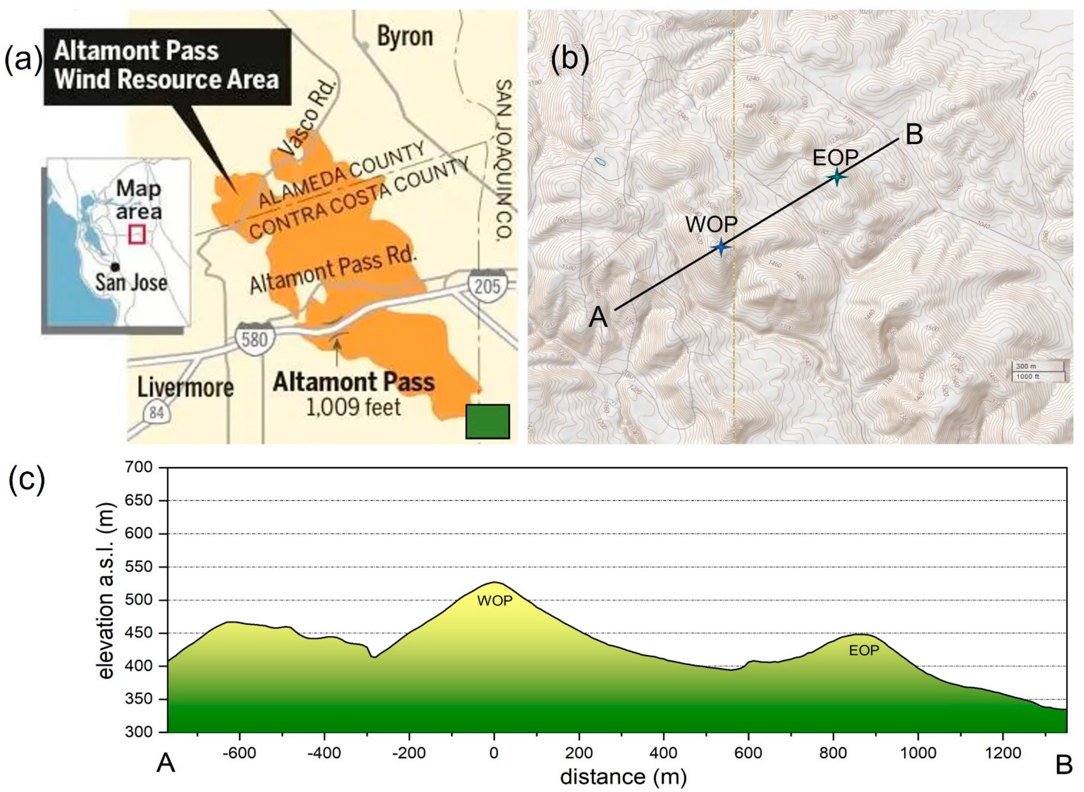
23]. HilFlowS wind profiles were collected from 12 July to 22 September by the student (K. Foster) on two ridgeline locations, referred to in this study as the West Observation Point (WOP) and the East Observation Point (EOP). Note that the name designations in this paper are different than the original designations in the DOE A2e dataset. WOP and EOP are separated by a line-of-sight distance of 860 m. WOP is the higher peak (527 m a.s.l. or 114 m a.g.l. based on the minimum upwind elevation) and one of the highest peaks in the immediate area. EOP is lower and reaches a height of 448 m a.s.l. or 54 m a.g.l. The average hill slope at WOP is 22° in the predominant wind direction. The gentler EOP hill has a slope of 13°. Additional hill characteristics for both ridgelines are shown in
Table 2. Inner and middle layer height estimates in
Table 2 are presented for near-neutral stability (see [
30] for methodology). A regional map, local topography, a terrain elevation profile are shown in
Figure 2.
Measurements of horizontal wind speed (U, m/s), vertical wind speed (w, m/s) and direction (°) were made using a ZephIR300 model vertically-profiling Doppler lidar (ZephIR Ltd., North Ledbury, UK). The two identical lidars were deployed along the predominant wind direction (240 deg) based on long-term, 52 m tall meteorological tower climatology at Site 300. The WOP and EOP lidars were set up identically with the exception of the power source. WOP had grid power access while the EOP lidar ran off of a solar panel/battery skid. This led to lower data recovery for the off-grid lidar. The WOP collected 1670 h of data; the EOP collected 1435 h. Only periods with data available at both lidars were examined in this analysis. Both lidars were deployed facing true north using multiple handheld GPS units as well as the on-board GPS unit. The alignment agreement was within +/− 1°. Data were downloaded weekly and analyzed by the undergraduate student to spot any possible issues with the data quality on a weekly basis.
ZephIR300 uses a velocity azimuth display (VAD) scanning mode (1 scan per second, 50 measurements per scan, 30° cone half-angle) to measure the wind profile up to 300 m (for more details see [
32]). During HilFlowS, the lidars were programmed to take measurements at 10, 20, 30, 38, 50, 60, 70, 80, 90, 120, 150 m above ground level. These heights cover most rotor-disk lengths at high resolution. The lidar has up to 10 programmable levels; 38 m is included as a standard calibration height. Because the lidars use coherent continuous-wave technology each level is not measured simultaneously, and is instead measured in series taking approximately 15 s to resample any given height. Probe depth (Δz) is not constant and increases with height. Δz ranges from 1.4 m at 10 m above ground level to 15.4 m at 100 m. The lidar also has an onboard 1 m meteorological station that collects observations of horizontal wind speed, direction, air pressure, air temperature and relative humidity. This allowed for a wind profile to be taken from 1 to 150 m during HilFlowS. The data are presented as ten-minute averages.
Atmospheric stability was estimated using a profile of air temperature and horizontal wind speed at Site 300’s 52 m tall meteorological tower to derive the bulk Richardson number (Rib) (see [
33] for methodology). Time periods were classified as stable, convective, or near-neutral depending on whether Rib was positive, negative, or near-zero, respectively. This largely corresponded to the hours of 21:00–6:00 local time classified as stable, 07:00–09:00 and 18:00–21:00 near-neutral, and 09:00–17:00 convective.
To evaluate lidar measurement accuracy an instrument cross-comparison was done over a period of six days prior to HilFlowS at the 52 m tall meteorological tower. At 40 m the cross-correlation between the two ZephIR lidars showed high agreement (Pearson’s r = 0.99, slope = 1.001 for wind direction; Pearson’s r = 0.99, slope = 1.001 for horizontal wind speed). All other heights of comparison had Pearson’s r values at 0.95 or above. Additional information about the ZephIR300 measurement technique and its use and uncertainties in complex terrain is found in [
10].
5. Results
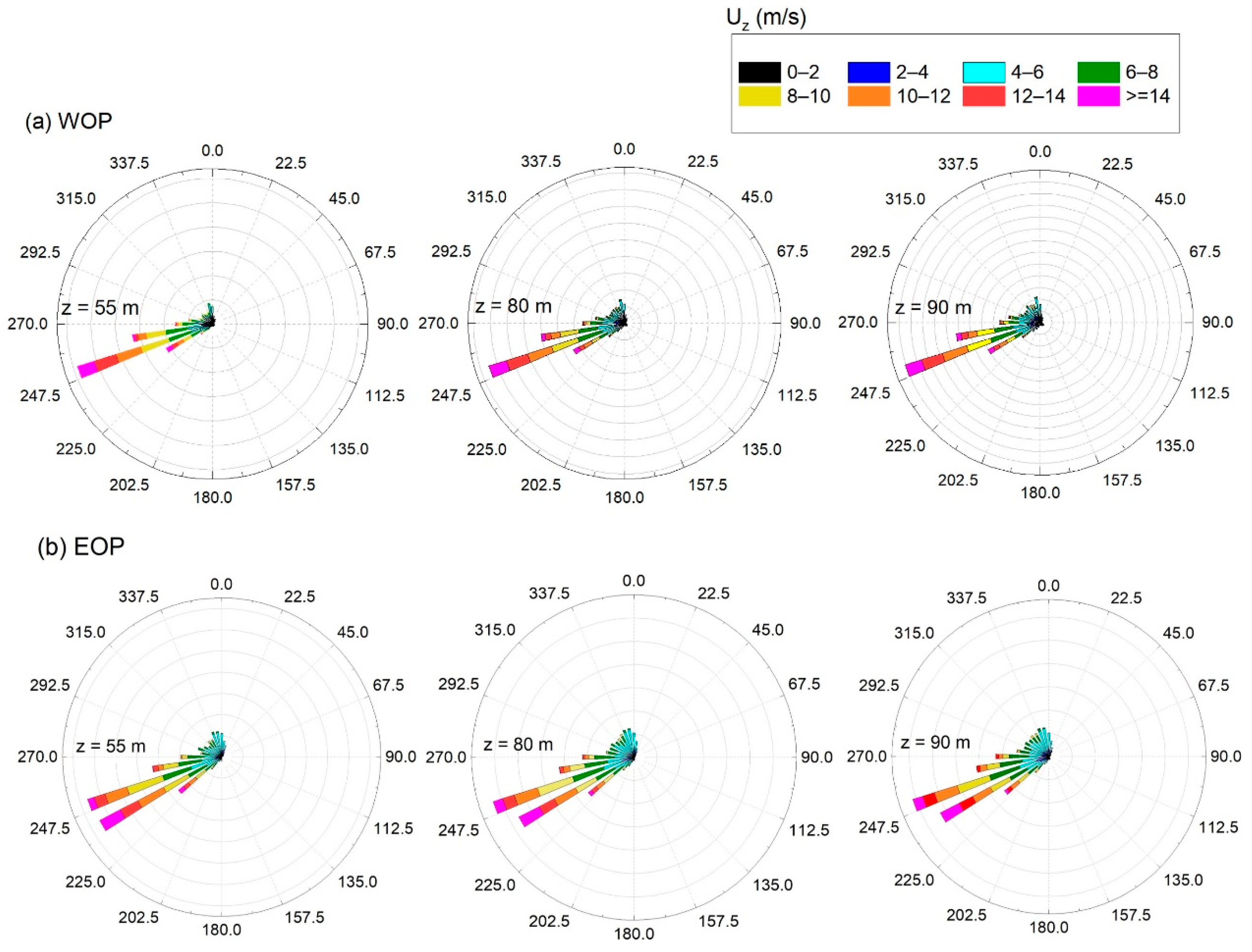
As expected, strong west-southwesterly winds were largely present during HilFlowS. These mostly occurred during stable, overnight hours but also were present around dawn and dusk (i.e., near-neutral conditions). Weaker, northerly winds were observed during some daylight hours during a convective, well-mixed atmosphere. Winds from other directions were largely absent during the campaign. The mean wind roses (these show the direction the wind is blowing from) were compiled for both locations at three heights: 50 m, 80 m, and 90 m (
Figure 3). These heights were chosen because they represent the three most common hub-heights in the repowered sections of the Altamont Pass. The data were center-binned into 7.5-degree sectors and all hours of the day are presented.
Figure 3 shows strongly channeled flow during the campaign at both WOP and EOP with very little difference observed between the two hill sites as seen in the wind roses. Less than 5% of all winds come from the 45°–180° sectors. The most common wind direction, west-southwesterly (230°–250°), has winds that hit normal to the ridgelines which acts to enhance the wind velocity, and wind speeds above 10 m/s were routinely measured on top of the hills. The wind roses also hint at the fact that wind velocity does not logarithmically increase with height, as seen by the lack of evidence of higher wind speeds at 90 m.
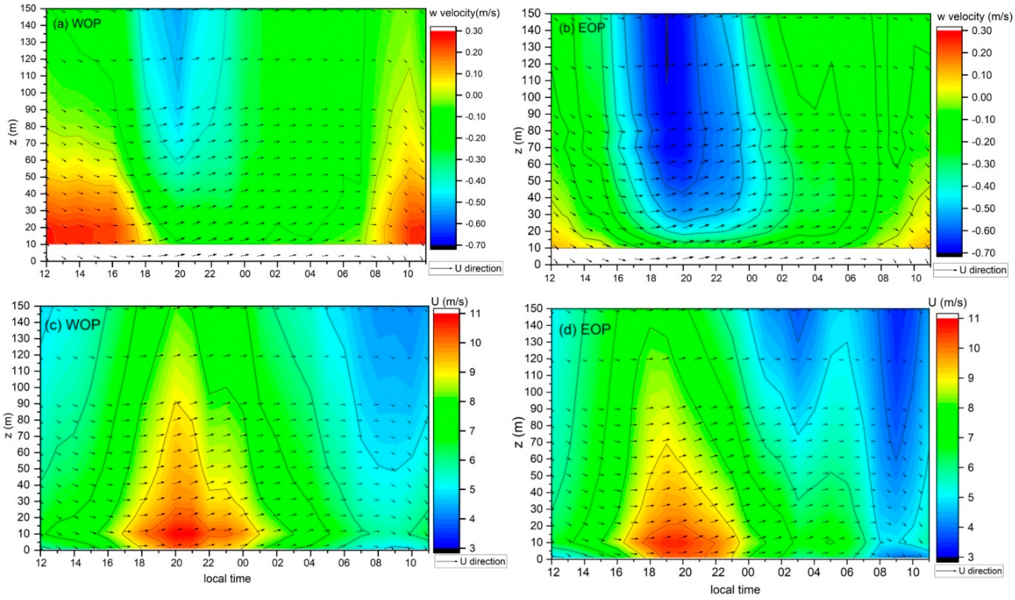
Because the time of day was highly correlated with stability class, diurnal plots are presented next to provide a higher temporal resolution look at the data versus separating it by a bulk Richardson stability bin. This was also done because the hill speed-up event covers both near-neutral and stable time periods. In order to look more closely at changes in wind speed with height and time of day, we examine mean diurnal plots in
Figure 4. On average, a wind maximum (Umax) of 10–11 m/s is observed to occur in the late afternoon leading to dissipation of the wind jet around midnight. This Umax or jet peaks in intensity between 1900 and 2100 local time, or just around sunset. Umax forms very close to the ground over both hills and peak winds occur between the heights of 1 and 20 m. Although this is well below hub-height, it does result in very large negative wind shear across heights equivalent to the rotor-disk. Note also that the larger rotor-disks extend down to almost 20 m off the ground as shown in
Figure 1. Umax appears to be associated with stronger subsidence from aloft as indicated by the large, negative vertical wind velocities found above the jet maxima. On average stronger subsidence is seen above the lower elevation, downwind hill.
Mean daytime (convective) northerly winds are much lower in intensity even at the highest 150 m measurement level and average around 6–8 m/s. Under these conditions, the flow is no longer normal to the ridgelines. A daily wind minimum at all heights is found around the hours of 800 to 1000 as the day begins warm and before the onshore-offshore pressure gradient develops and intensifies. Mean wind direction is also shown as vectors in
Figure 4. Except for the morning hours which correspond with slower northerly winds, wind direction is largely constant with the time of day and by height and blows from the west-southwest (i.e., onshore winds).
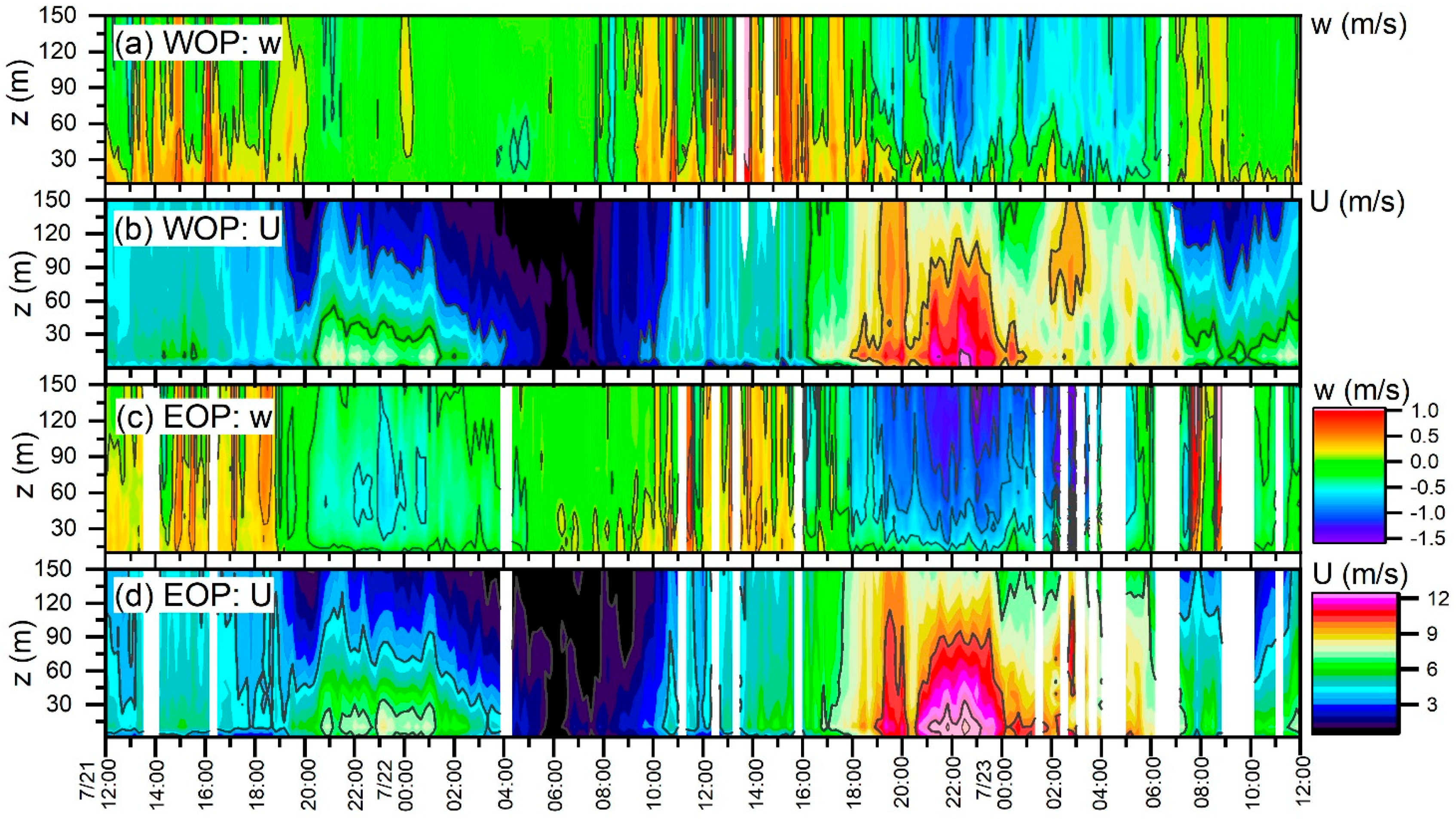
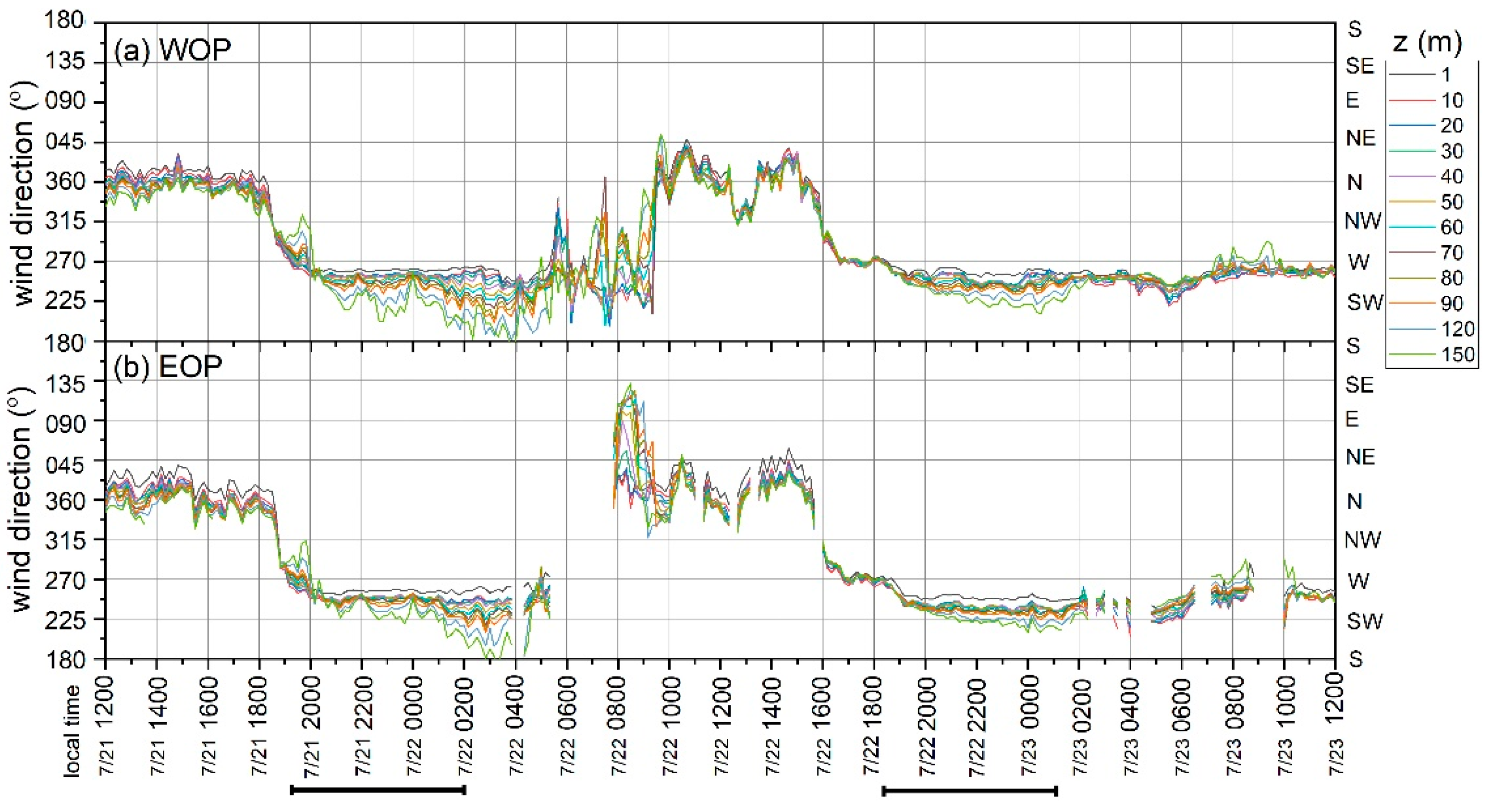
To examine Umax in greater detail two back-to-back wind maxima events are shown in
Figure 5 for the nights of 21–22 and 22–23 July. The figure shows that while the timing of the hill-speed up flows is similar on both nights, the intensity of the maxima peaks on the second night. On these days, Umax is also strongest at the lower EOP hill which coincides with stronger subsidence (
Figure 5a,c) and less veer (
Figure 6). Both are factors that produce strong channeled flow close to the surface. In fact, higher veer is observed on the (weaker Umax) first night at both sites. Here we can see the winds turn counterclockwise with height, until the time when the veer reaches a maximum and the wind velocity jet is fully dissipated.
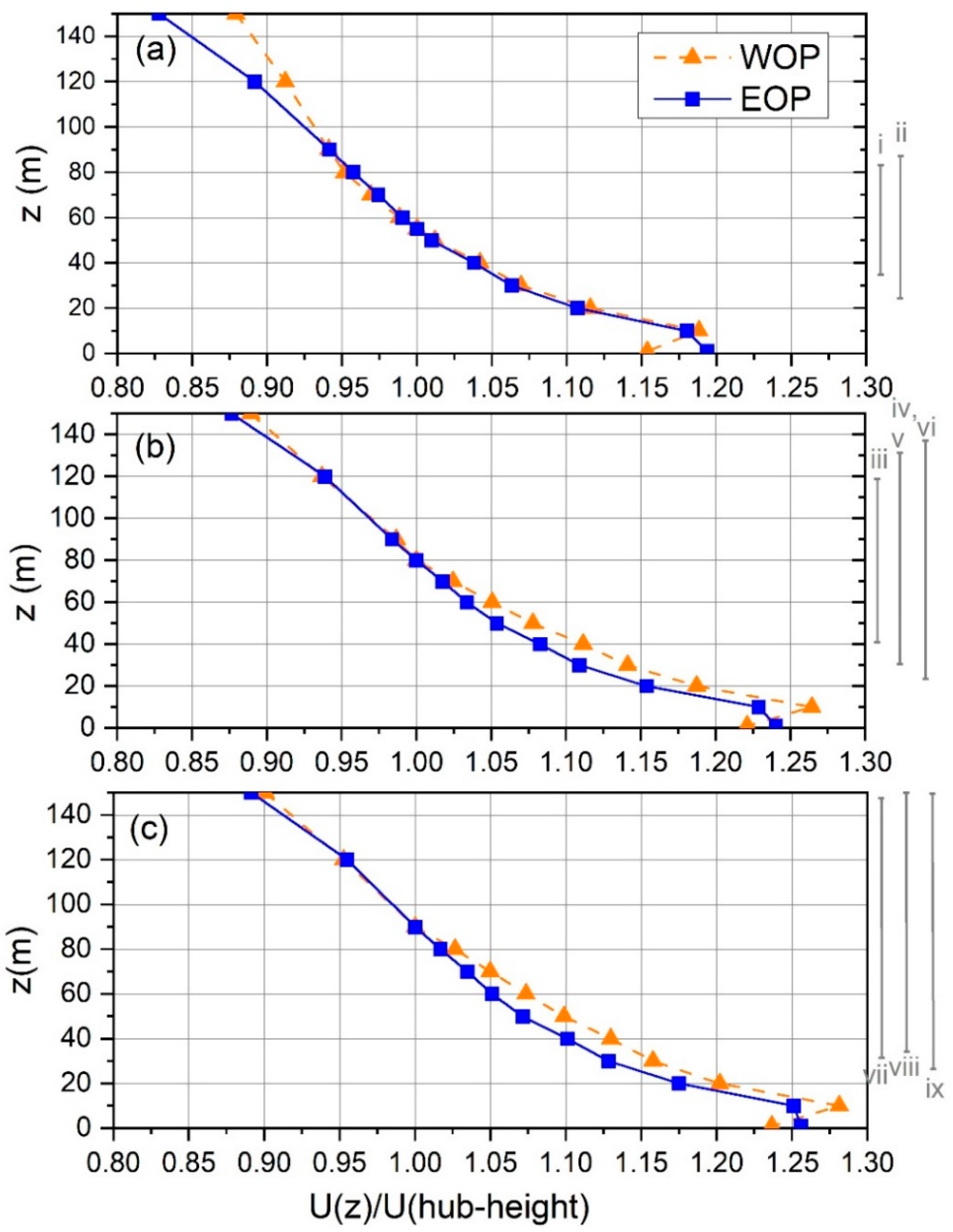
To aid in comparing the WOP and EOP wind profiles and assess the wind resource available to a turbine,
Figure 7 shows the mean wind speed normalized by wind speed found at three hub-heights: 55 m, 80 m and 90 m. These include only times when the hub-height wind direction is normal to the ridgelines. While we saw a stronger wind maximum at the EOP for a couple of isolated days in
Figure 5, the mean normalized profiles show that the wind maximum is strongest at the steeper, windward WOP hill. At WOP, Umax occurs roughly at 10 m, or somewhere between 1 and 20 m a.g.l. But without highly detailed measurements it’s impossible to know the exact height, and magnitude, of the wind maximum. At EOP, the wind maximum was found closer to the ground and probably occurred somewhere around 1 to 10 m a.g.l., but again lack of higher resolution measurements may have missed the true Umax. These heights are in agreement with where the theorized wind maximum should occur for near-neutral conditions (
Table 2, inner layer depth).
Figure 7 also highlights all of the altitudes where air would interact with a wind turbine depending on the turbine’s make and model. Here, we see that the turbines are going to fluctuate from being in the middle layer (depth of 50–55 m) to the outer atmospheric layer (>≈60 m) depending on atmospheric stability and the turbine blades do not reach down to the inner layer (<10 m). While all of the turbine disks miss the actual Umax it is important to note that the wind jets observed during HilFlowS occur at wind speeds (average = 10–11 m/s) that are important for turbine power generation. A typical turbine has a cut-in speed of 2–3 m/s, a rated speed of 12–15 m/s, and a cut-out speed of 25 m/s. For wind speeds between cut-in speed and rated speed, turbine power extraction is proportional to the wind speed cubed (as measured across the rotor diameter). Hence, the higher wind speeds seen in the bottom half of the turbine rotor disks are right in the “sweet-spot” of the power curve for maximizing power generation.
A wind shear parameter (α) is sometimes used to extrapolate the wind speed taken at a reference height (usually the hub-height nacelle anemometer) to all other heights in the rotor disk when those wind speeds are not known. Historically, a constant α-value of 0.14 is used to represent average atmospheric boundary layer conditions [
34], but this value is only valid under certain conditions (i.e., near-neutral stability, flat, homogeneous terrain, low surface roughness, etc.). Our observations show wind shear parameters are very different from 0.14 and α increases (becomes more strongly negative) with increasing turbine hub-height. At WOP, the average rotor-disk α-value is −0.10 for hub-height = 55 m, −0.14 for hub-height = 80 m, and −0.15 for hub-height = 90 m. At EOP, α ranges from −0.11 for hub-height = 55 m, −0.15 for hub-height = 80 m, and −0.17 for hub-height = 90 m. What is remarkable is that these strongly negative wind shear parameter values were largely observed during stable or near-neutral conditions. Under stable conditions, α is expected to become more positive, as we see for conditions in flat northern Oklahoma, where α-values of +0.2 to +0.3 are routinely seen [
33]. The impacts of a strong, negative wind shear on power generation (e.g., via increased fatigue loads) certainly warrants further attention as taller turbines are replacing shorter models in the APWRA. The authors encourage readers interested in turbine controls and power modeling to download the HilFlowS wind profiles from the DOE A2e data portal.
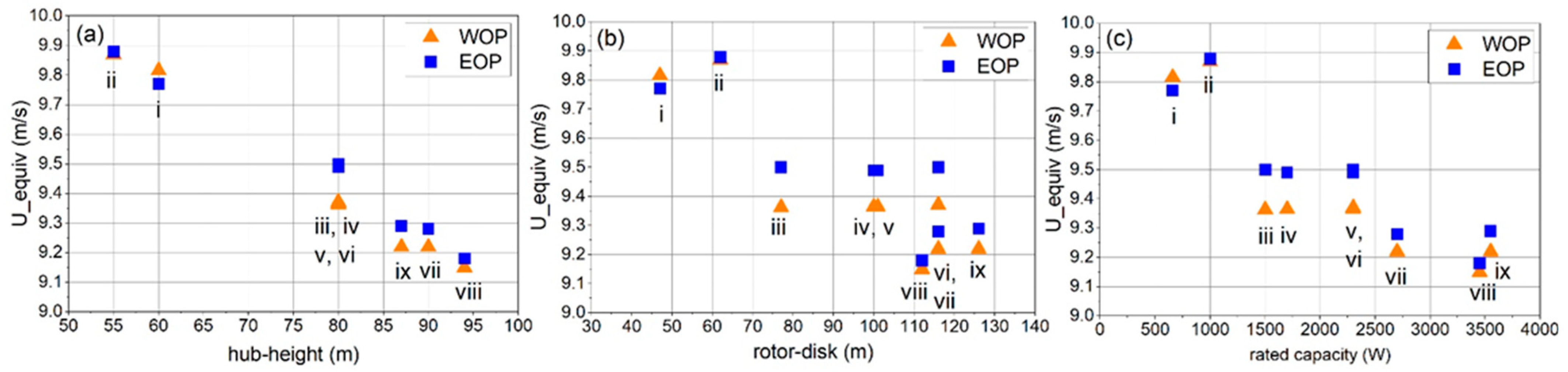
Given these large values of wind shear, we look next at the rotor-disk equivalent wind speed (Uequiv, m/s) to see how it compares to hub-height wind speed. Under high shear conditions, Uequiv is largely accepted to be a better representation of the true wind speed found across the entire rotor-disk (e.g., [
35]). Because of the large differences in turbine rated capacity due to re-powering in the Altamont, we concentrate on comparing Uequiv for turbines with similar power classes (refer to
Figure 1).
Figure 8 shows the mean Uequiv magnitudes observed over WOP and EOP as a function of (
Figure 8a) hub-height, (
Figure 8b) rotor diameter, and (
Figure 8c) rated capacity for the nine evaluated turbines. WOP and EOP have very similar Uequiv values and location differences are usually 0.1 m/s or less. The most obvious finding is that the shorter turbines encounter a stronger wind resource at both locations. This is caused by the height of Umax (as discussed previously) and the large wind shear values which create strong winds closer to the ground surface than at heights aloft. Interestingly, Uequiv is less correlated with rotor disk length. Again, this is because rotor disk length is not directly correlated with hub-height. Altamont turbines vi (GE2.3-116) and viii (GE2.7-116) provide excellent examples of this. While both have rotor diameters of 116 m and are close in rated capacity, the 80 m tall GE2.3-116 would have access to a larger wind resource based on our data than the taller (90 m) model. On the other hand, four of the turbines (iii–vi) have identical hub-heights (80 m), but their rotor-disk lengths range from 77 m to 116 m. In this case, we see little difference in Uequiv across turbine models.
The findings during HilFlowS agree with summertime profiles taken in 2017 and in earlier years at Site 300. Winds normal to the ridgelines at Site 300 show a wind maximum close to the surface and negative shear aloft, while winds parallel to the ridgelines show a more standard wind profile with winds increasing with height (i.e., positive shear). Because wind direction at Site 300 is highly seasonal (synoptically driven northerly winds in the winter and synoptically driven south-westerly winds in the summer), the wind profiles also vary in a similar way by season [
23]. So while we don’t see strong hill-speed up flows in the winter, that period of time also coincides with an overall weaker wind resource in the area.
To assess the relative strength of summer-time, terrain-induced flow acceleration in the Altamont we look at two other ridge experiments for comparison: Cooper’s Ridge and Perdigão. Cooper’s Ridge was a tower-based campaign in Australia that captured mean wind flow over an isolated, 115 m tall (10° slope) ridge with low surface roughness [
7]. Perdigão, a more recent experiment, was an intensively instrumented field experiment conducted across two ~200 m tall, parallel ridgelines in Portugal [
12,
20]. In terms of land cover, Cooper’s Ridge is very similar to HilFlowS; both experiments were done in regions covered with uniform short grasslands with low surface roughness. However, unlike HilFlowS, Cooper’s Ridge is a relatively isolated feature in the landscape. At Perdigão the landscape was more heterogenous in terms of surrounding land use and vegetation than HilFlowS and the ridges are taller, but the studies are similar in that they examined flow over parallel ridgelines.
At Cooper’s Ridge, Umax was observed to be strong and low to the ground (<10 m) under near-neutral and stable conditions. There, a hill-speed up factor (Δs) of two was found in stable conditions. Although HilFlowS does not have the upwind profile to calculate Δs we suspect that Δs would also be high in the summer in the Altamont given the strong Umax values observed over the tops of the hills. Wind profiles on top of the Perdigão ridgelines showed that the upwind hill has a Umax occurring around 20 m a.g.l., and at the downward hill Umax was found around 30 a.g.l. [
36]. These heights are in rough agreement with the inner layer estimates calculated by [
37] for the site. Perdigão U maxima were overall was much smaller in magnitude than observed during the peak wind season HilFlowS experiment and a Perdigão Umax was not significantly greater than winds measured at 80 m hub-height suggesting a weaker Δs within the rotor-disk, at least during that experiment’s duration, than we observed in the Altamont.


