
Assessment of ANN Algorithms for the Concentration Prediction of Indoor Air Pollutants in Child Daycare Centers


Abstract
:1. Introduction
2. Machine Learning Applications for the Prediction of Indoor Air Quality
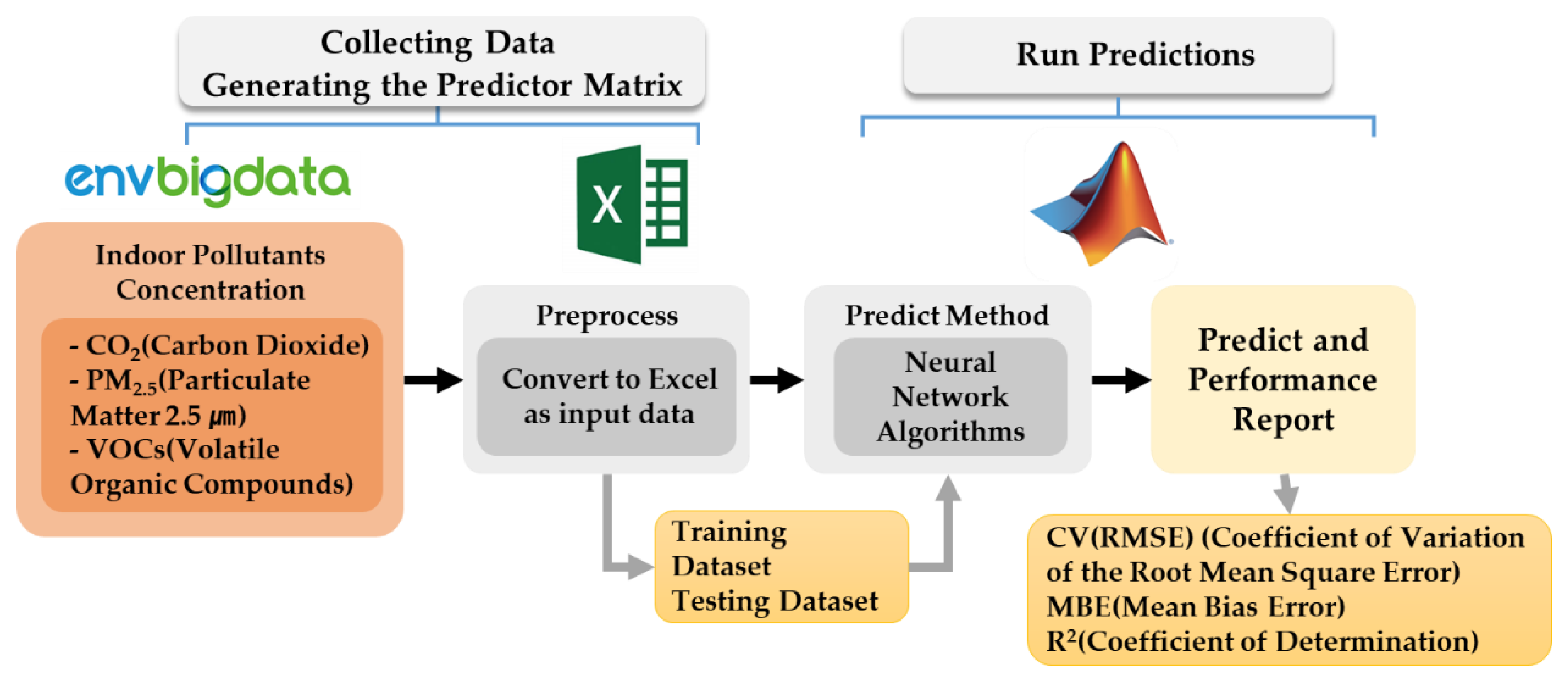
3. Methodology
3.1. Collection of Training Data Set
3.2. Indoor Pollutant Concentration Prediction Model
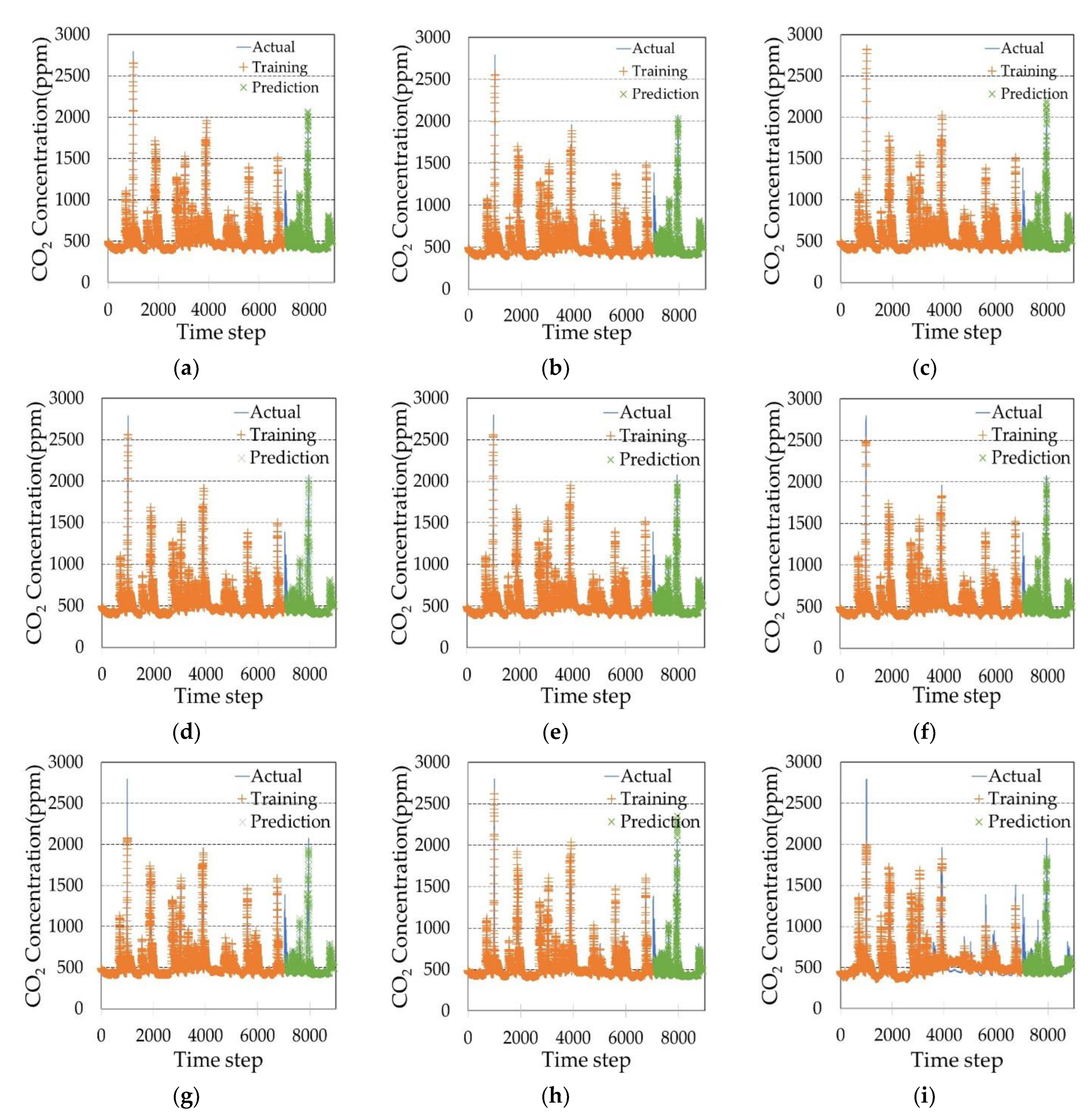
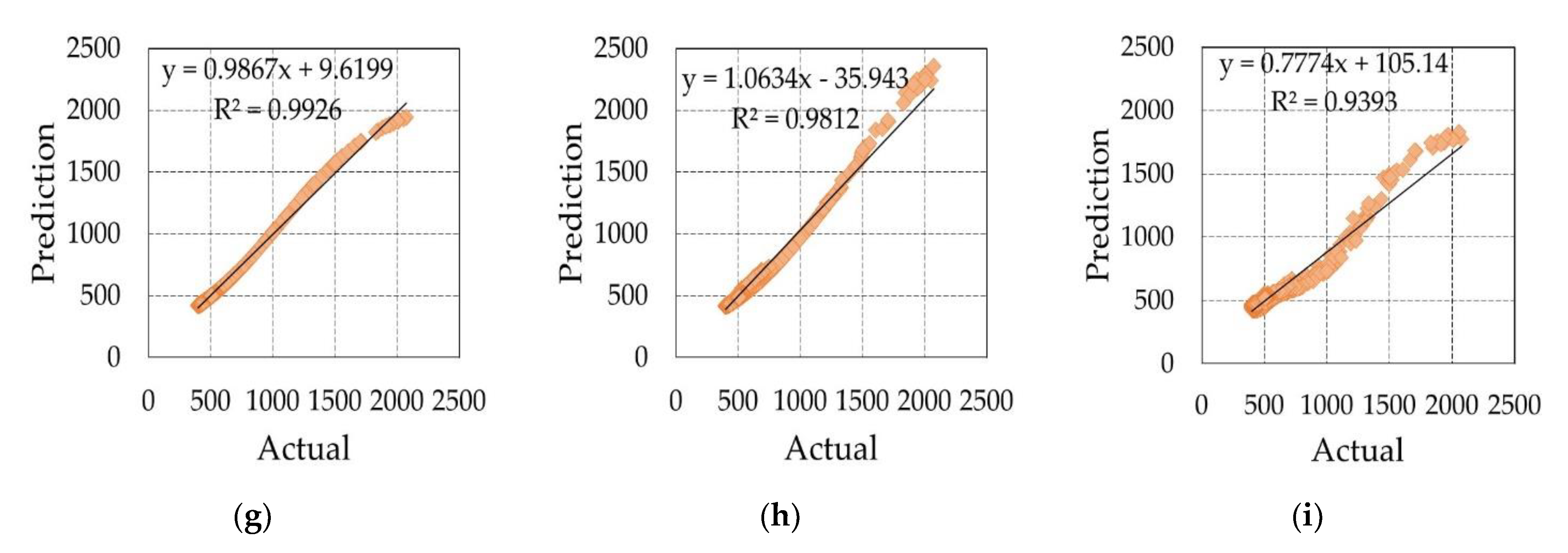
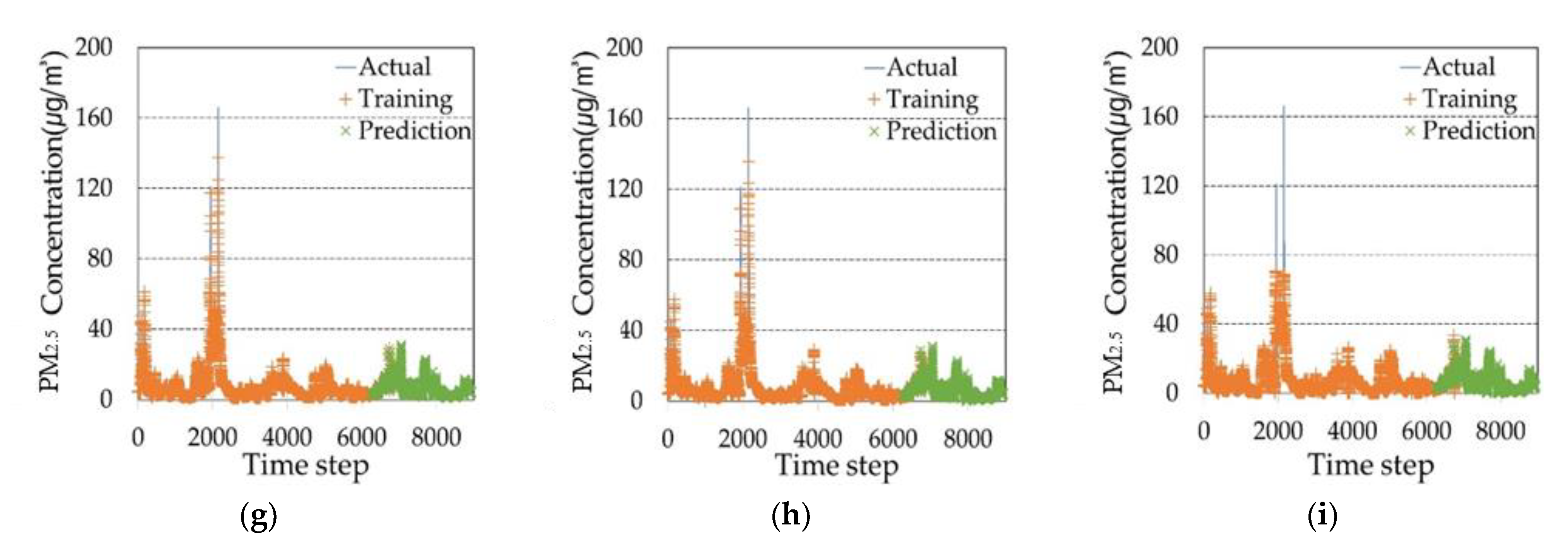
4. Results
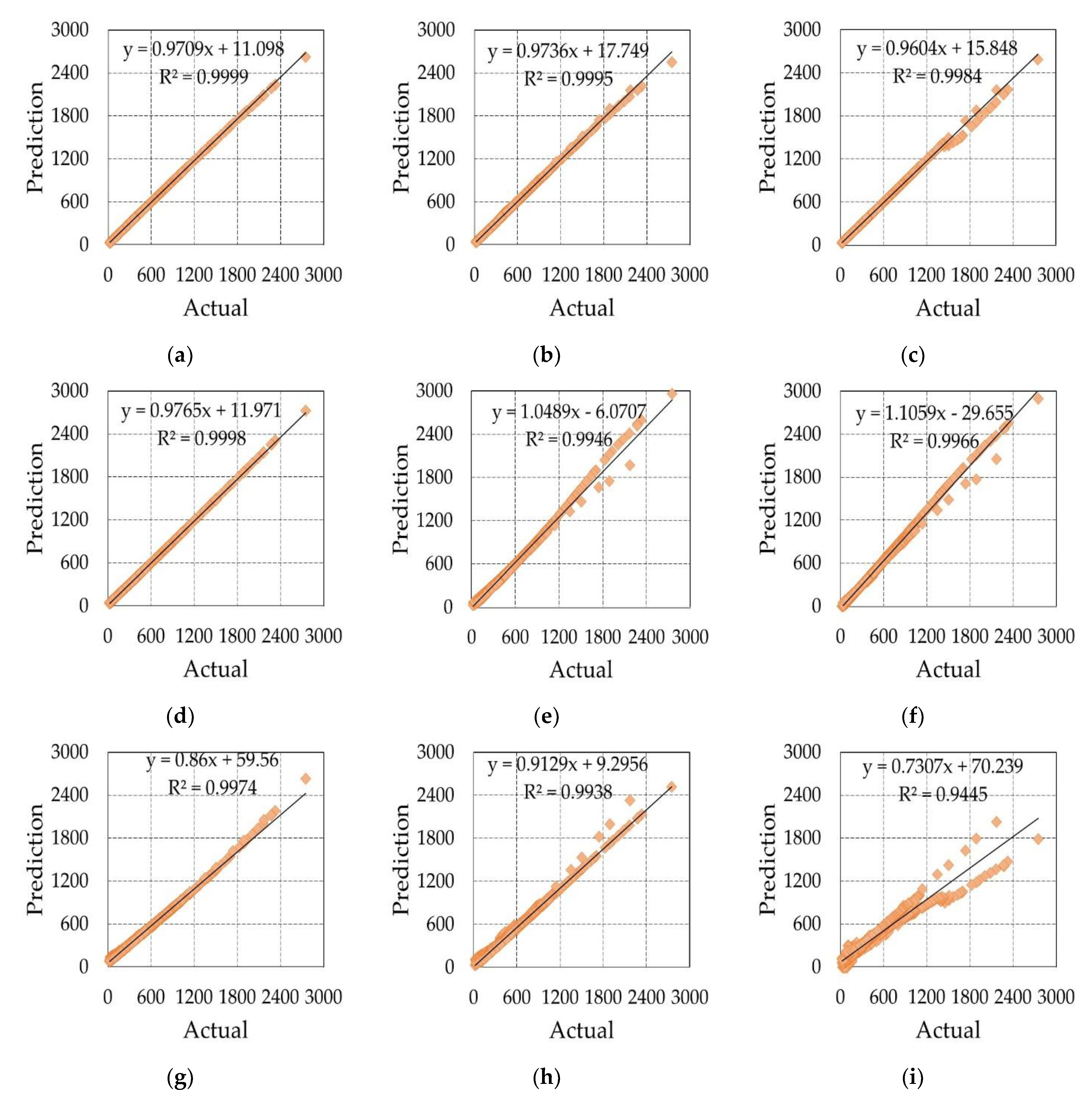
4.1. CO2
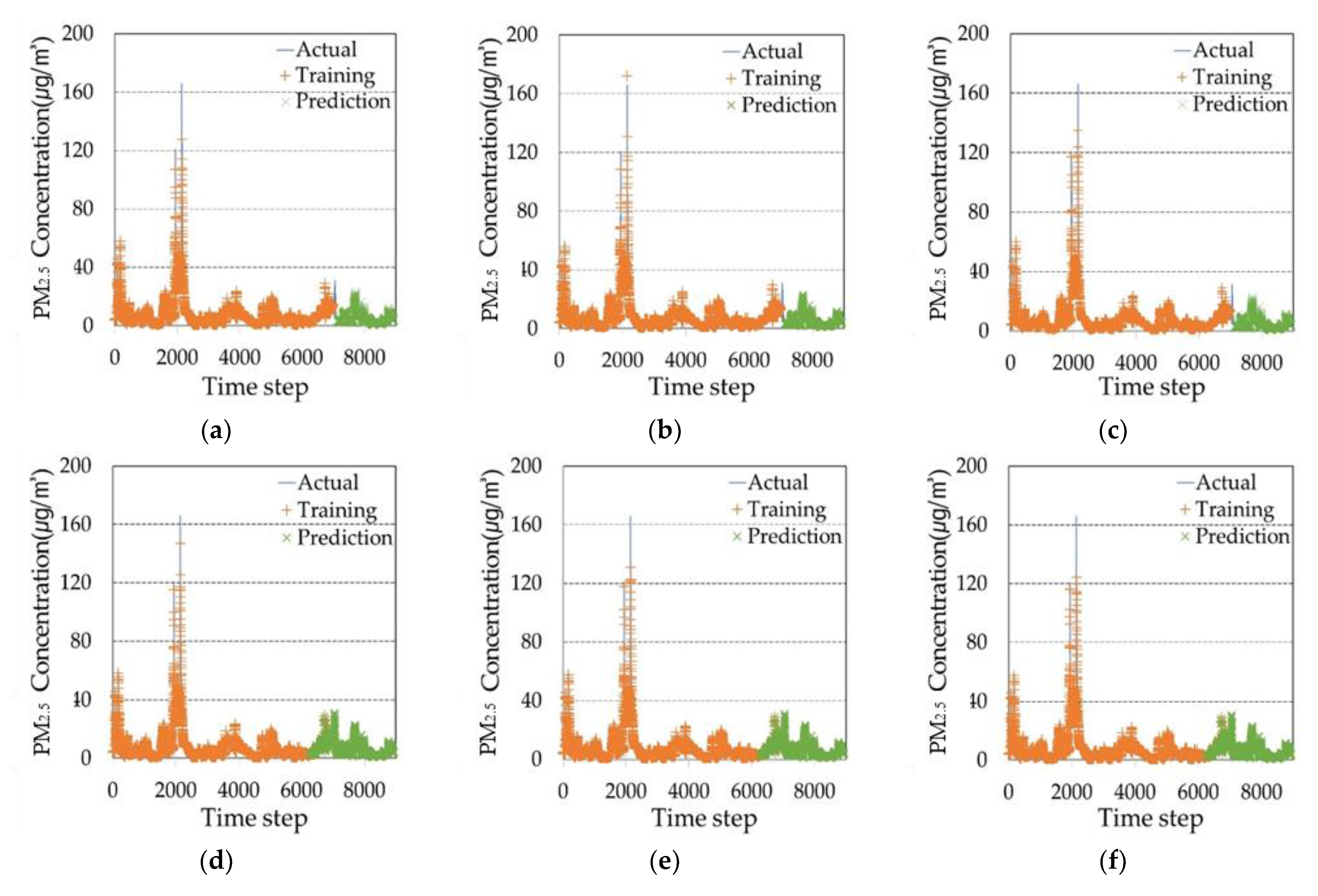
4.2. PM2.5
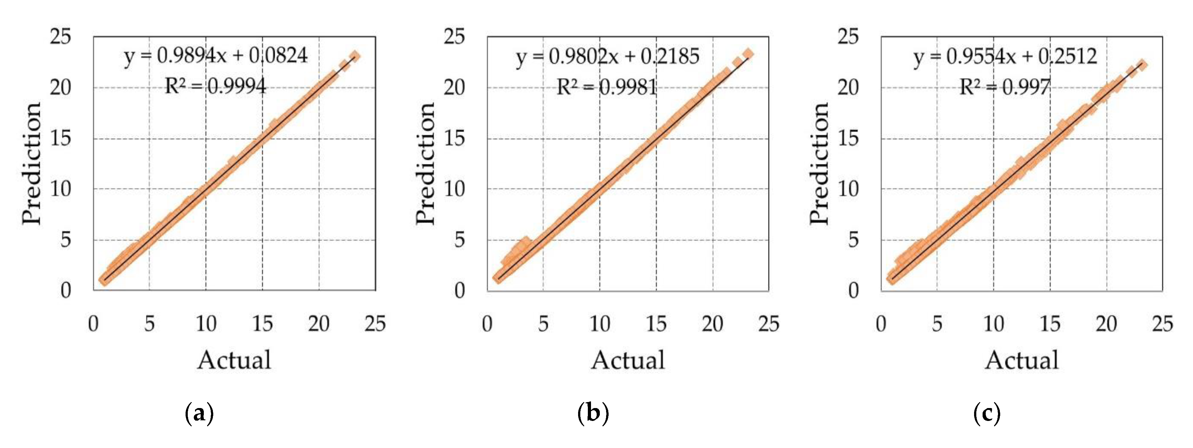
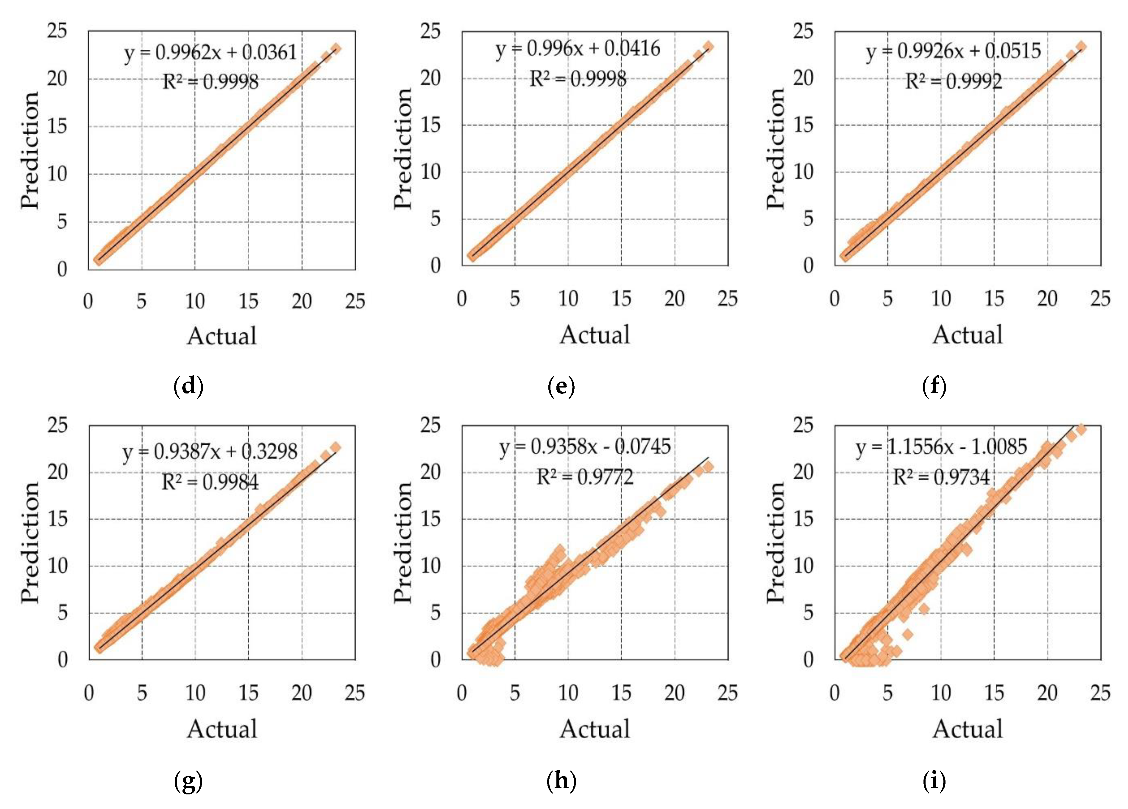
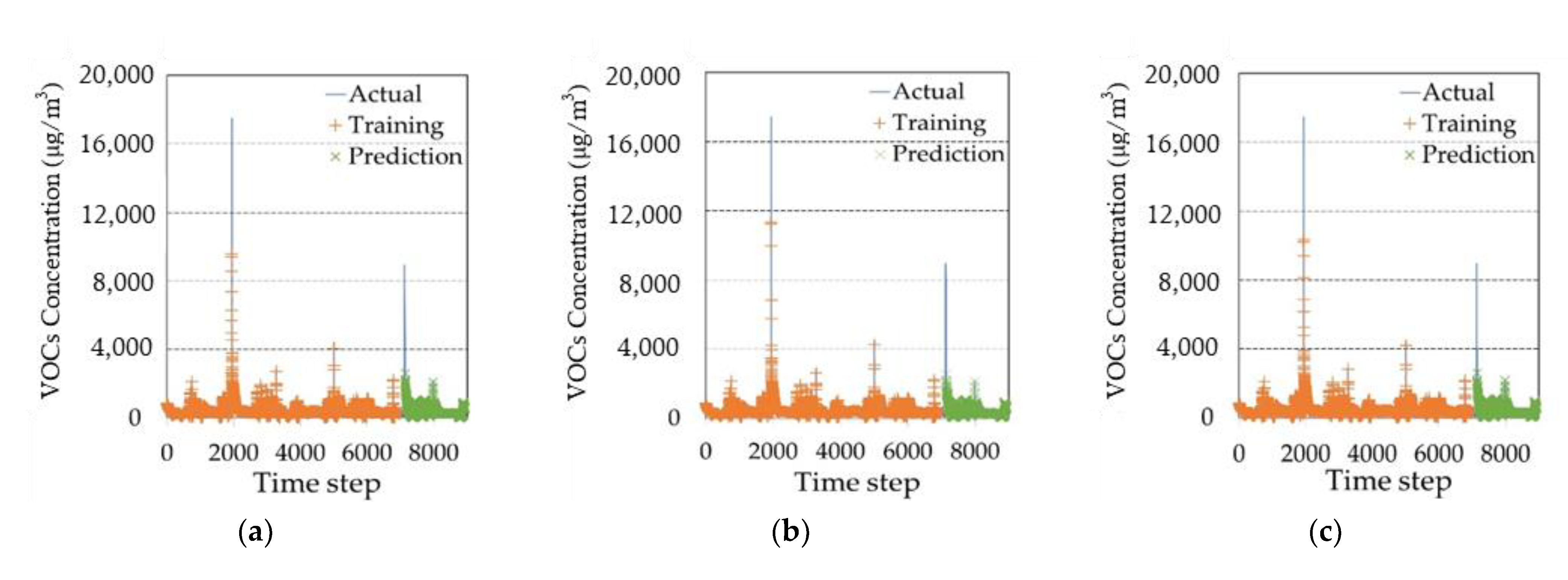
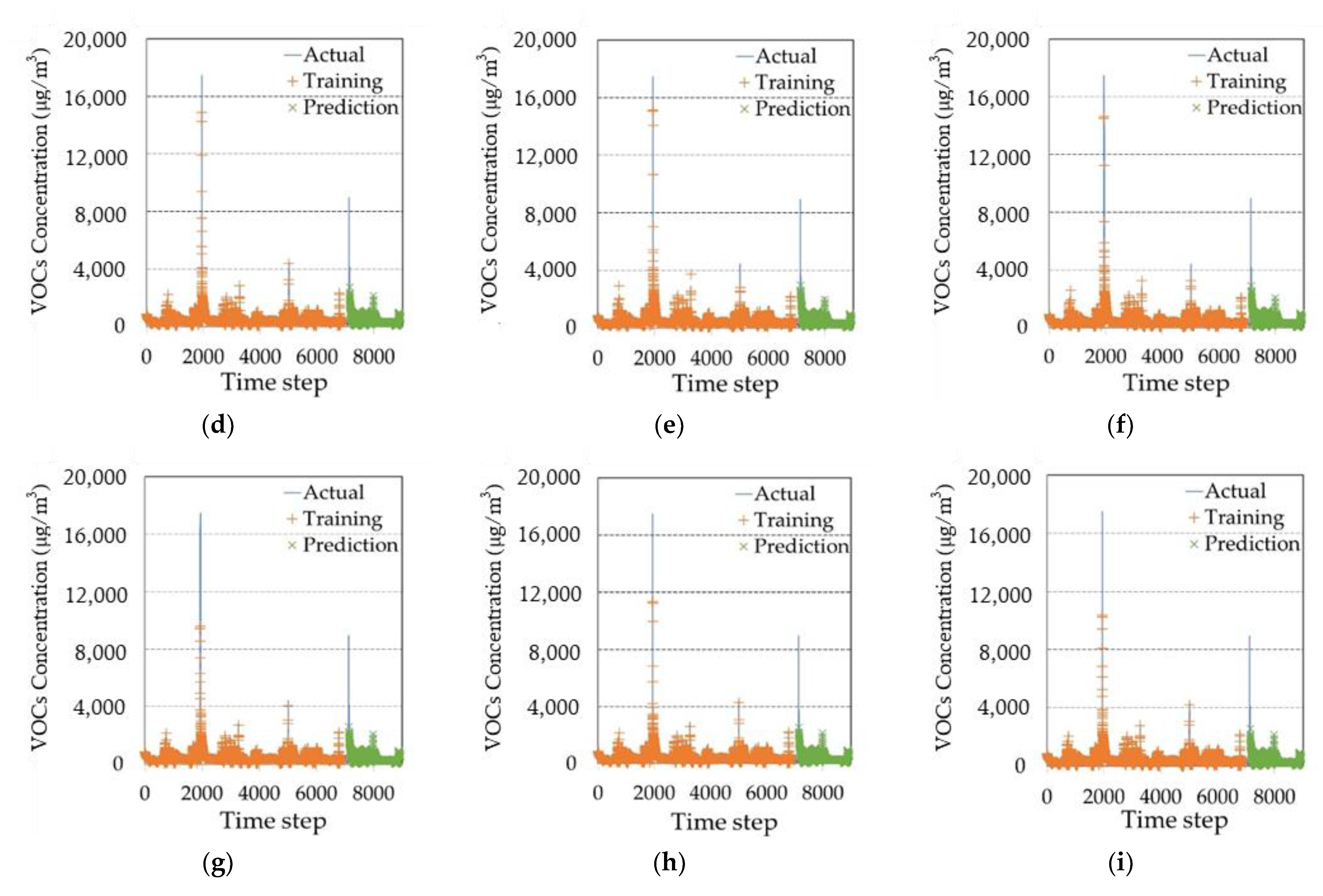
4.3. VOCs
5. Discussion
6. Conclusions
Author Contributions
Funding
Institutional Review Board Statement
Informed Consent Statement
Data Availability Statement
Conflicts of Interest
References
- Awada, M.; Becerik-Gerber, B.; Hoque, S.; O’Neill, Z.; Pedrielli, G.; Wen, J.; Wu, T. Ten questions concerning occupant health in buildings during normal operations and extreme events including the COVID-19 pandemic. Build. Environ. 2021, 188, 107480. [Google Scholar] [CrossRef]
- Adam, M.G.; Tran, P.T.M.; Balasubramanian, R. Air quality changes in cities during the COVID-19 lockdown: A critical review. Atmos. Res. 2021, 264, 105823. [Google Scholar] [CrossRef] [PubMed]
- Schibuola, L.; Tambani, C. High energy efficiency ventilation to limit COVID-19 contagion in school environments. Energy Build. 2021, 240, 110882. [Google Scholar] [CrossRef] [PubMed]
- Sha, H.; Zhang, X.; Qi, D. Optimal control of high-rise building mechanical ventilation system for achieving low risk of COVID-19 transmission and ventilative cooling. Sustain. Cities Soc. 2021, 74, 103256. [Google Scholar] [CrossRef]
- Gil-Baez, M.; Lizana, J.; Becerra Villanueva, J.A.; Molina-Huelva, M.; Serrano-Jimenez, A.; Chacartegui, R. Natural ventilation in classrooms for healthy schools in the COVID era in mediterranean climate. Build. Environ. 2021, 206, 108345. [Google Scholar] [CrossRef]
- Szczepanik-Ścisło, N.; Ścisło, Ł. Air leakage modelling and its influence on the air quality inside a garage. E3S Web Conf. 2018, 44, 00172. [Google Scholar] [CrossRef] [Green Version]
- Ye, W.; Won, D.; Zhang, X. A preliminary ventilation rate determination methods study for residential buildings and offices based on voc emission database. Build. Environ. 2014, 79, 168–180. [Google Scholar] [CrossRef]
- Földváry, V.; Bekö, G.; Langer, S.; Arrhenius, K.; Petráš, D. Effect of energy renovation on indoor air quality in multifamily residential buildings in slovakia. Build. Environ. 2017, 122, 363–372. [Google Scholar] [CrossRef] [Green Version]
- Kaunelienė, V.; Prasauskas, T.; Krugly, E.; Stasiulaitienė, I.; Čiužas, D.; Šeduikytė, L.; Martuzevičius, D. Indoor air quality in low energy residential buildings in lithuania. Build. Environ. 2016, 108, 63–72. [Google Scholar] [CrossRef]
- Yang, S.; Yuk, H.; Yun, B.Y.; Kim, Y.U.; Wi, S.; Kim, S. Passive pm2.5 control plan of educational buildings by using airtight improvement technologies in south korea. J. Hazard. Mater. 2022, 423, 126990. [Google Scholar] [CrossRef]
- Bralewska, K.; Rogula-Kozłowska, W.; Bralewski, A. Indoor air quality in sports center: Assessment of gaseous pollutants. Build. Environ. 2022, 208, 108589. [Google Scholar] [CrossRef]
- Connolly, R.E.; Yu, Q.; Wang, Z.; Chen, Y.-H.; Liu, J.Z.; Collier-Oxandale, A.; Papapostolou, V.; Polidori, A.; Zhu, Y. Long-term evaluation of a low-cost air sensor network for monitoring indoor and outdoor air quality at the community scale. Sci. Total Environ. 2022, 807, 150797. [Google Scholar] [CrossRef]
- Mikola, A.; Hamburg, A.; Kuusk, K.; Kalamees, T.; Voll, H.; Kurnitski, J. The impact of the technical requirements of the renovation grant on the ventilation and indoor air quality in apartment buildings. Build. Environ. 2022, 210, 108698. [Google Scholar] [CrossRef]
- Kang, I.; McCreery, A.; Azimi, P.; Gramigna, A.; Baca, G.; Abromitis, K.; Wang, M.; Zeng, Y.; Scheu, R.; Crowder, T.; et al. Indoor air quality impacts of residential mechanical ventilation system retrofits in existing homes in chicago, il. Sci. Total Environ. 2022, 804, 150129. [Google Scholar] [CrossRef]
- Al-Rawi, M.; Ikutegbe, C.A.; Auckaili, A.; Farid, M.M. Sustainable technologies to improve indoor air quality in a residential house—A case study in waikato, new zealand. Energy Build. 2021, 250, 111283. [Google Scholar] [CrossRef]
- Oh, H.-J.; Nam, I.-S.; Yun, H.; Kim, J.; Yang, J.; Sohn, J.-R. Characterization of indoor air quality and efficiency of air purifier in childcare centers, korea. Build. Environ. 2014, 82, 203–214. [Google Scholar] [CrossRef]
- Roda, C.; Barral, S.; Ravelomanantsoa, H.; Dusséaux, M.; Tribout, M.; Le Moullec, Y.; Momas, I. Assessment of indoor environment in paris child day care centers. Environ. Res. 2011, 111, 1010–1017. [Google Scholar] [CrossRef]
- Hwang, S.H.; Seo, S.; Yoo, Y.; Kim, K.Y.; Choung, J.T.; Park, W.M. Indoor air quality of daycare centers in seoul, korea. Build. Environ. 2017, 124, 186–193. [Google Scholar] [CrossRef]
- Madureira, J.; Paciência, I.; Rufo, J.C.; Pereira, C.; Teixeira, J.P.; de Oliveira Fernandes, E. Assessment and determinants of airborne bacterial and fungal concentrations in different indoor environments: Homes, child day-care centres, primary schools and elderly care centres. Atmos. Environ. 2015, 109, 139–146. [Google Scholar] [CrossRef] [Green Version]
- St-Jean, M.; St-Amand, A.; Gilbert, N.L.; Soto, J.C.; Guay, M.; Davis, K.; Gyorkos, T.W. Indoor air quality in montréal area day-care centres, canada. Environ. Res. 2012, 118, 1–7. [Google Scholar] [CrossRef]
- Harbizadeh, A.; Mirzaee, S.A.; Khosravi, A.D.; Shoushtari, F.S.; Goodarzi, H.; Alavi, N.; Ankali, K.A.; Rad, H.D.; Maleki, H.; Goudarzi, G. Indoor and outdoor airborne bacterial air quality in day-care centers (dccs) in greater ahvaz, iran. Atmos. Environ. 2019, 216, 116927. [Google Scholar] [CrossRef]
- Zuraimi, M.S.; Tham, K.W. Indoor air quality and its determinants in tropical child care centers. Atmos. Environ. 2008, 42, 2225–2239. [Google Scholar] [CrossRef]
- Araújo-Martins, J.; Carreiro Martins, P.; Viegas, J.; Aelenei, D.; Cano, M.M.; Teixeira, J.P.; Paixão, P.; Papoila, A.L.; Leiria-Pinto, P.; Pedro, C.; et al. Environment and health in children day care centres (envirh)—Study rationale and protocol. Rev. Port. De Pneumol. 2014, 20, 311–323. [Google Scholar] [CrossRef] [PubMed] [Green Version]
- Heibati, S.; Maref, W.; Saber, H.H. Assessing the energy, indoor air quality, and moisture performance for a three-story building using an integrated model, part two: Integrating the indoor air quality, moisture, and thermal comfort. Energies 2021, 14, 4915. [Google Scholar] [CrossRef]
- Olu-Ajayi, R.; Alaka, H.; Sulaimon, I.; Sunmola, F.; Ajayi, S. Machine learning for energy performance prediction at the design stage of buildings. Energy Sustain. Dev. 2022, 66, 12–25. [Google Scholar] [CrossRef]
- Elbeltagi, E.; Wefki, H. Predicting energy consumption for residential buildings using ann through parametric modeling. Energy Rep. 2021, 7, 2534–2545. [Google Scholar] [CrossRef]
- Olu-Ajayi, R.; Alaka, H.; Sulaimon, I.; Sunmola, F.; Ajayi, S. Building energy consumption prediction for residential buildings using deep learning and other machine learning techniques. J. Build. Eng. 2022, 45, 103406. [Google Scholar] [CrossRef]
- Zhu, Y.F.; Yao, Y.; Huang, Y.; Chen, C.H.; Zhang, H.Y.; Huang, Z. Machine learning applications for assessment of dynamic progressive collapse of steel moment frames. Structures 2022, 36, 927–934. [Google Scholar] [CrossRef]
- Chalapathy, R.; Khoa, N.L.D.; Sethuvenkatraman, S. Comparing multi-step ahead building cooling load prediction using shallow machine learning and deep learning models. Sustain. Energy Grids Netw. 2021, 28, 100543. [Google Scholar] [CrossRef]
- Ding, Y.; Fan, L.; Liu, X. Analysis of feature matrix in machine learning algorithms to predict energy consumption of public buildings. Energy Build. 2021, 249, 111208. [Google Scholar] [CrossRef]
- Zhang, H.; Srinivasan, R.; Yang, X. Simulation and analysis of indoor air quality in florida using time series regression (tsr) and artificial neural networks (ann) models. Symmetry 2021, 13, 952. [Google Scholar] [CrossRef]
- Amuthadevi, C.; Ds, V.; Ramachandran, V. Development of air quality monitoring (aqm) models using different machine learning approaches. J. Ambient Intell. Humaniz. Comput. 2021, 1–13. [Google Scholar] [CrossRef]
- Tagliabue, L.C.; Re Cecconi, F.; Rinaldi, S.; Ciribini, A.L.C. Data driven indoor air quality prediction in educational facilities based on iot network. Energy Build. 2021, 236, 110782. [Google Scholar] [CrossRef]
- Jang, H.-S.; Xing, S. A model to predict ammonia emission using a modified genetic artificial neural network: Analyzing cement mixed with fly ash from a coal-fired power plant. Constr. Build. Mater. 2020, 230, 117025. [Google Scholar] [CrossRef]
- Jeong, J.-H.; Jo, J.-H.; Kim, S.-H.; Bang, S.-H.; Lee, S.-S. A study on machine learning model for predicting uncollected parameters in indoor environment evaluation. J. Korea Inst. Inf. Electron. Commun. Technol. 2021, 14, 413–420. [Google Scholar]
- Scislo, L.; Szczepanik-Scislo, N. Air quality sensor data collection and analytics with iot for an apartment with mechanical ventilation. In Proceedings of the 2021 11th IEEE International Conference on Intelligent Data Acquisition and Advanced Computing Systems: Technology and Applications (IDAACS), Cracow, Poland, 22–25 September 2021; pp. 932–936. [Google Scholar]
- Li, Z.; Tong, X.; Ho, J.M.W.; Kwok, T.C.Y.; Dong, G.; Ho, K.-F.; Yim, S.H.L. A practical framework for predicting residential indoor pm2.5 concentration using land-use regression and machine learning methods. Chemosphere 2021, 265, 129140. [Google Scholar] [CrossRef] [PubMed]
- Kallio, J.; Tervonen, J.; Räsänen, P.; Mäkynen, R.; Koivusaari, J.; Peltola, J. Forecasting office indoor co2 concentration using machine learning with a one-year dataset. Build. Environ. 2021, 187, 107409. [Google Scholar] [CrossRef]
- Taheri, S.; Razban, A. Learning-based co2 concentration prediction: Application to indoor air quality control using demand-controlled ventilation. Build. Environ. 2021, 205, 108164. [Google Scholar] [CrossRef]
- Sassi, M.S.H.; Fourati, L.C. In Deep learning and augmented reality for iot-based air quality monitoring and prediction system. In Proceedings of the 2021 International Symposium on Networks, Computers and Communications (ISNCC), Dubai, United Arab Emirates, 31 October–2 November 2021; pp. 1–6. [Google Scholar]
- Saad, S.M.; Andrew, A.M.; Shakaff, A.Y.M.; Saad, A.R.M.; Kamarudin, A.M.Y.; Zakaria, A. Classifying sources influencing indoor air quality (iaq) using artificial neural network (ann). Sensors 2015, 15, 11665–11684. [Google Scholar] [CrossRef] [Green Version]
- Putra, J.C.P.; Safrilah; Ihsan, M. The prediction of indoor air quality in office room using artificial neural network. AIP Conf. Proc. 2018, 1977, 020040. [Google Scholar]
- Dai, X.; Liu, J.; Zhang, X.; Chen, W. An artificial neural network model using outdoor environmental parameters and residential building characteristics for predicting the nighttime natural ventilation effect. Build. Environ. 2019, 159, 106139. [Google Scholar] [CrossRef]
- Segala, G.; Doriguzzi Corin, R.; Peroni, C.; Gazzini, T.; Siracusa, D. A practical and adaptive approach to predicting indoor co2. Appl. Sci. 2021, 11, 10771. [Google Scholar] [CrossRef]
- Big Data Environment Platform. Available online: https://www.Bigdata-environment.Kr/user/main.Do (accessed on 1 November 2021).
- Matlab, The Mathworks, Inc. Available online: https://www.Mathworks.Com/?S_tid=gn_logo (accessed on 1 December 2021).
- Golafshani, E.M.; Behnood, A. Application of soft computing methods for predicting the elastic modulus of recycled aggregate concrete. J. Clean. Prod. 2018, 176, 1163–1176. [Google Scholar] [CrossRef]
- Koçer, M.; Öztürk, M.; Hakan Arslan, M. Determination of moment, shear and ductility capacities of spiral columns using an artificial neural network. J. Build. Eng. 2019, 26, 100878. [Google Scholar] [CrossRef]
- Wang, R.; Lu, S.; Li, Q. Multi-criteria comprehensive study on predictive algorithm of hourly heating energy consumption for residential buildings. Sustain. Cities Soc. 2019, 49, 101623. [Google Scholar] [CrossRef]
- American Society of Heating, Refrigerating and Air Conditioning Engineers. Ashrae Guideline 14-2002, Measurement of Energy and Demand Savings—Measurement of Energy, Demand and Water Savings. 2002. Available online: http://www.eeperformance.org/uploads/8/6/5/0/8650231/ashrae_guideline_14-2002_measurement_of_energy_and_demand_saving.pdf (accessed on 1 February 2021).
- Bui, D.-K.; Nguyen, T.N.; Ngo, T.D.; Nguyen-Xuan, H. An artificial neural network (ann) expert system enhanced with the electromagnetism-based firefly algorithm (efa) for predicting the energy consumption in buildings. Energy 2020, 190, 116370. [Google Scholar] [CrossRef]
- Lu, C.; Li, S.; Lu, Z. Building energy prediction using artificial neural networks: A literature survey. Energy Build. 2022, 262, 111718. [Google Scholar] [CrossRef]
- Yeon, S.; Yu, B.; Seo, B.; Yoon, Y.; Lee, K.H. Ann based automatic slat angle control of venetian blind for minimized total load in an office building. Sol. Energy 2019, 180, 133–145. [Google Scholar] [CrossRef]
- Cho, J.H.; Moon, J.W. Integrated artificial neural network prediction model of indoor environmental quality in a school building. J. Clean. Prod. 2022, 344, 131083. [Google Scholar] [CrossRef]


| Parameter | Value | |
|---|---|---|
| Number of hidden layers | 1, 3, 5 | |
| Number of neurons | 20 | |
| Epochs | 100 | |
| Data | Training | 7142 (80%) |
| Testing | 1785 (20%) | |
| Calibration Type | Index | ASHRAE Guideline 14 [50] |
|---|---|---|
| Monthly | MBE_monthly | ±5% |
| CvRMSE_monthly | 15% | |
| Hourly | MBE_hourly | ±10% |
| CvRMSE_hourly | 30% |
| Training Algorithm | Hidden Layers-1 | Hidden Layers-3 | Hidden Layers-5 | |||
|---|---|---|---|---|---|---|
| CV(RMSE) (%) | MBE (%) | CV(RMSE) (%) | MBE (%) | CV(RMSE) (%) | MBE (%) | |
| LM | 4.04 | 7.53 | 4.06 | 8.03 | 4.47 | 8.56 |
| BR | 4.06 | 7.53 | 4.15 | 7.98 | 4.21 | 8.06 |
| BFG | 5.26 | 9.86 | 7.65 | 10.16 | 12.54 | 10.86 |
| Training Algorithm | Hidden Layers-1 | Hidden Layers-3 | Hidden Layers-5 | |||
|---|---|---|---|---|---|---|
| CV(RMSE) (%) | MBE (%) | CV(RMSE) (%) | MBE (%) | CV(RMSE) (%) | MBE (%) | |
| LM | 13.24 | 4.44 | 13.76 | 5.17 | 13.73 | 5.49 |
| BR | 13.17 | 3.62 | 13.27 | 3.91 | 13.31 | 4.25 |
| BFG | 13.79 | 5.66 | 18.60 | 6.52 | 27.90 | 6.69 |
| Training Algorithm | Hidden Layers-1 | Hidden Layers-3 | Hidden Layers-5 | |||
|---|---|---|---|---|---|---|
| CV(RMSE) (%) | MBE (%) | CV(RMSE) (%) | MBE (%) | CV(RMSE) (%) | MBE (%) | |
| LM | 10.81 | 8.89 | 10.98 | 9.35 | 11.12 | 8.96 |
| BR | 11.06 | 9.10 | 14.11 | 10.19 | 15.65 | 10.37 |
| BFG | 14.57 | 10.68 | 14.58 | 10.79 | 26.52 | 11.25 |
Publisher’s Note: MDPI stays neutral with regard to jurisdictional claims in published maps and institutional affiliations. |
© 2022 by the authors. Licensee MDPI, Basel, Switzerland. This article is an open access article distributed under the terms and conditions of the Creative Commons Attribution (CC BY) license (https://creativecommons.org/licenses/by/4.0/).
Share and Cite
Kim, J.; Hong, Y.; Seong, N.; Kim, D.D. Assessment of ANN Algorithms for the Concentration Prediction of Indoor Air Pollutants in Child Daycare Centers. Energies 2022, 15, 2654. https://doi.org/10.3390/en15072654
Kim J, Hong Y, Seong N, Kim DD. Assessment of ANN Algorithms for the Concentration Prediction of Indoor Air Pollutants in Child Daycare Centers. Energies. 2022; 15(7):2654. https://doi.org/10.3390/en15072654
Chicago/Turabian StyleKim, Jeeheon, Yongsug Hong, Namchul Seong, and Daeung Danny Kim. 2022. "Assessment of ANN Algorithms for the Concentration Prediction of Indoor Air Pollutants in Child Daycare Centers" Energies 15, no. 7: 2654. https://doi.org/10.3390/en15072654
APA StyleKim, J., Hong, Y., Seong, N., & Kim, D. D. (2022). Assessment of ANN Algorithms for the Concentration Prediction of Indoor Air Pollutants in Child Daycare Centers. Energies, 15(7), 2654. https://doi.org/10.3390/en15072654