
White-Model Predictive Control for Balancing Energy Savings and Thermal Comfort


Abstract
:1. Introduction
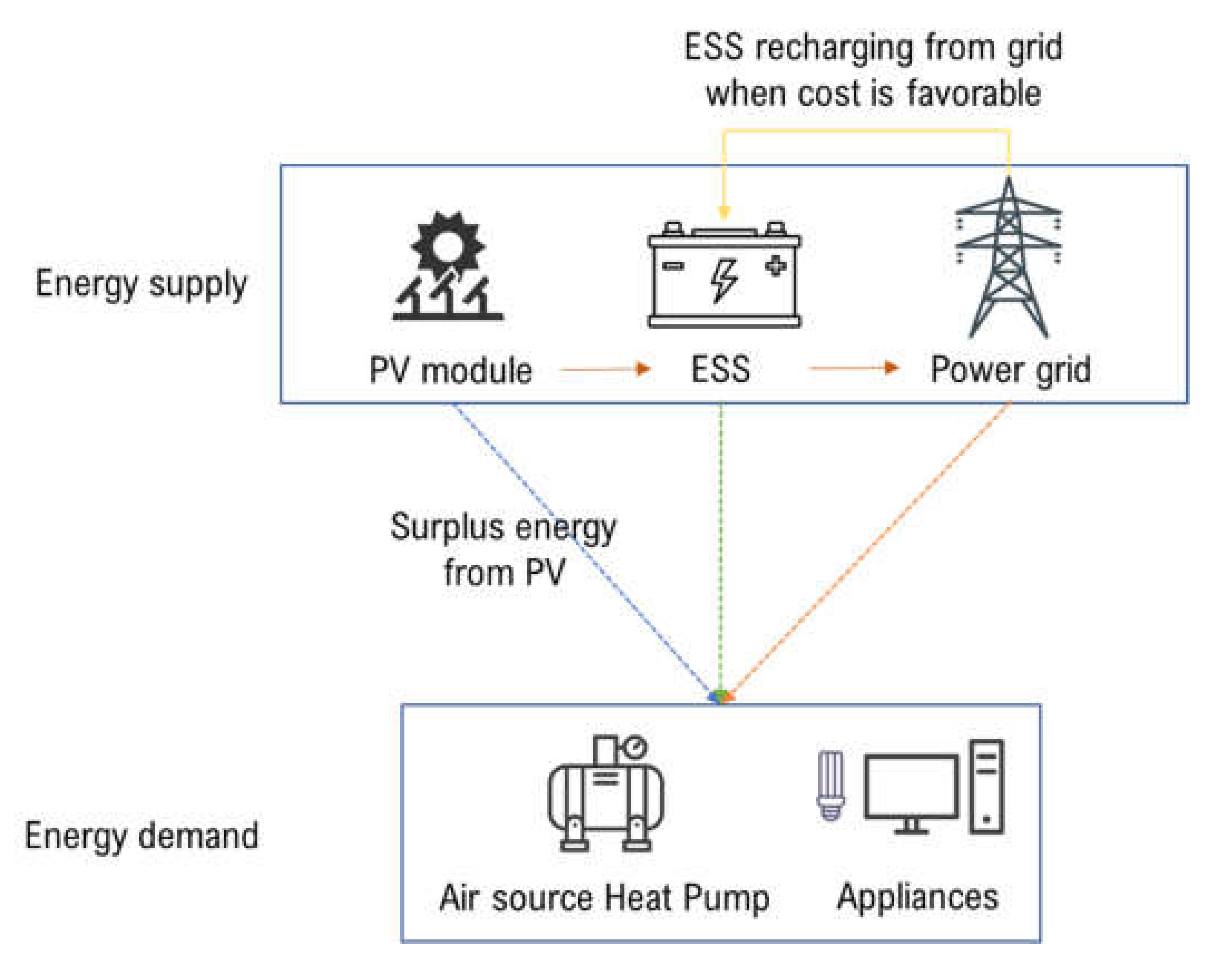
2. Target Simulation Models
3. Multi-Objective Optimal Control Strategy
3.1. Genetic Algorithm
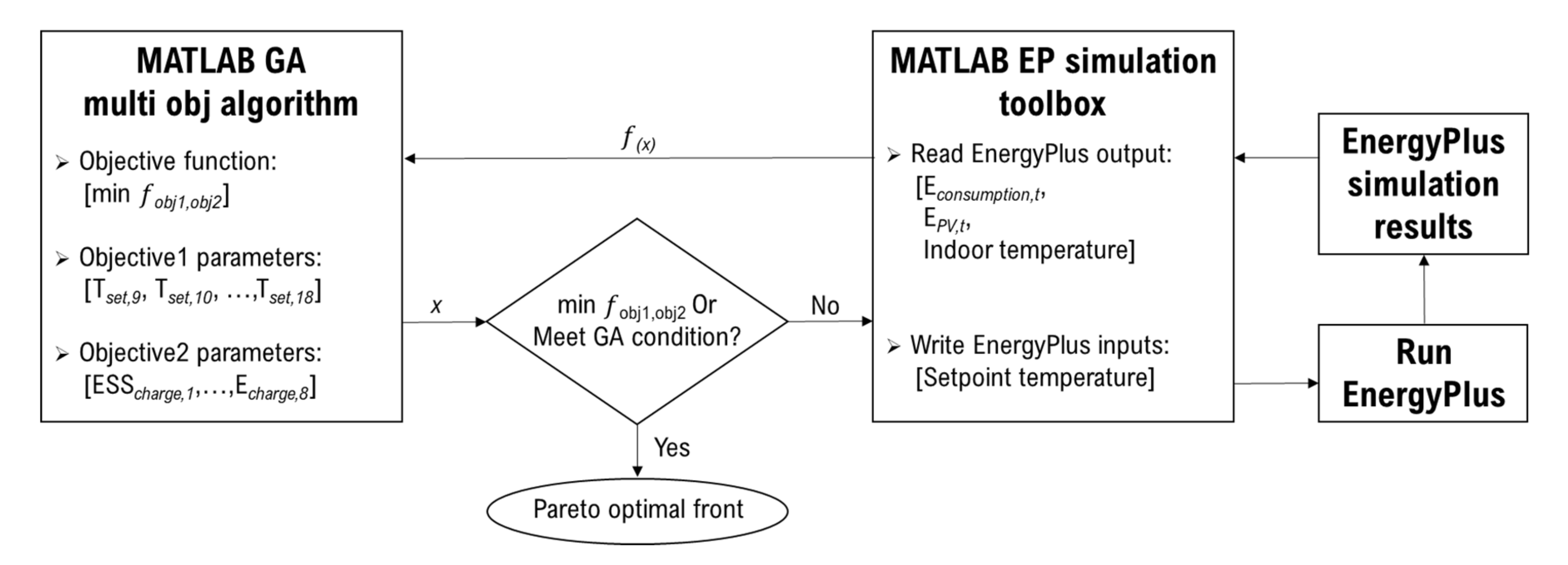
3.2. Coupling EnergyPlus and MATLAB
3.3. Objective Function
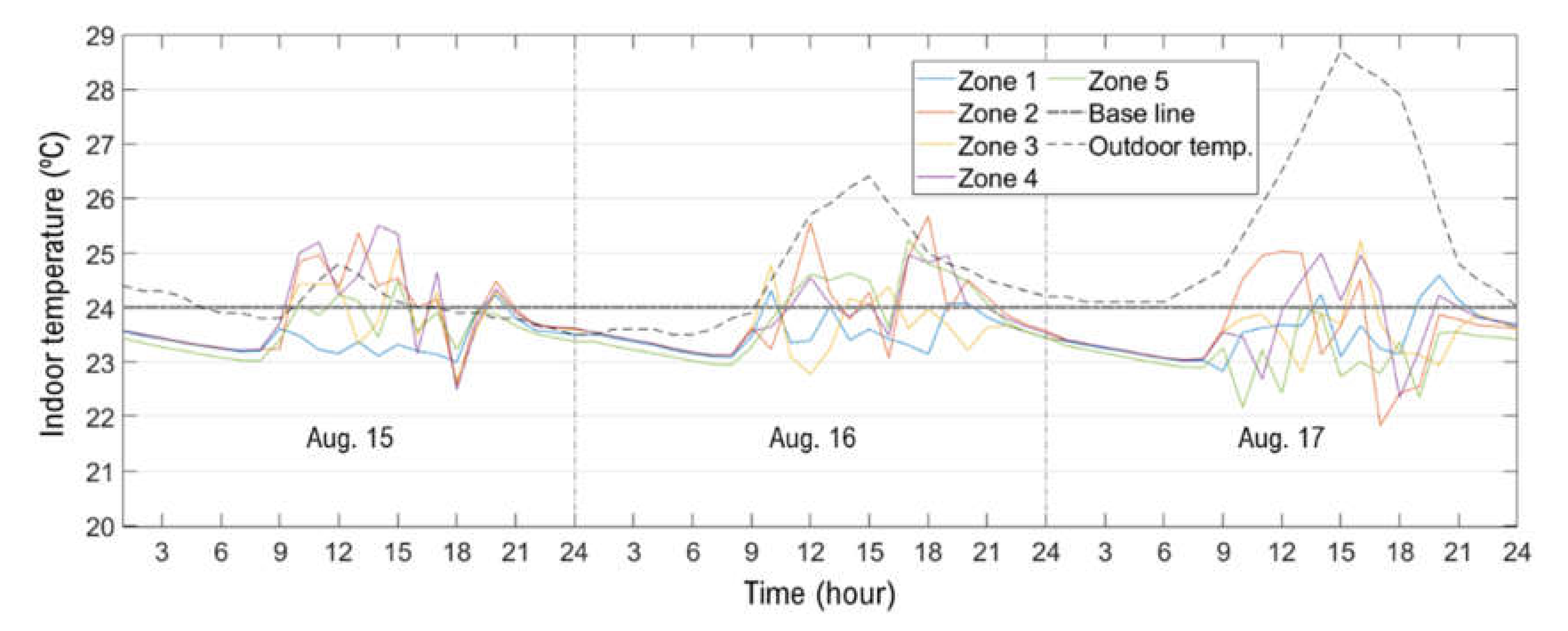
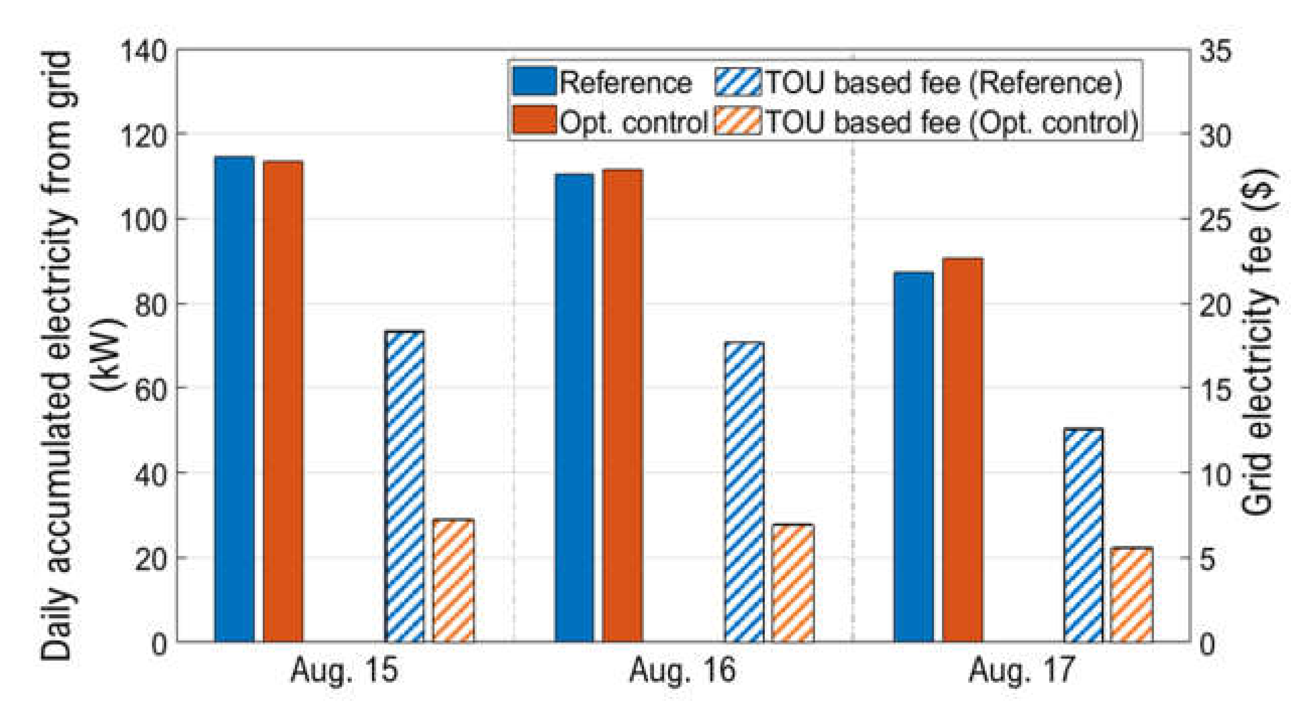
4. Optimization Results
5. Conclusions
Author Contributions
Funding
Institutional Review Board Statement
Informed Consent Statement
Data Availability Statement
Conflicts of Interest
References
- Doe, U. Buildings Energy Data Book; Energy Efficiency & Renewable Energy Department: Washington, DC, USA, 2011. [Google Scholar]
- Drgoňa, J.; Arroyo, J.; Cupeiro Figueroa, I.C.; Blum, D.; Arendt, K.; Kim, D.; Ollé, E.P.; Oravec, J.; Wetter, M.; Vrabie, D.L.; et al. All You Need to Know About Model Predictive Control for Buildings. Annu. Rev. Control. 2020, 50, 190–232. [Google Scholar] [CrossRef]
- Freire, R.Z.; Oliveira, G.H.C.; Mendes, N. Predictive Controllers for Thermal Comfort Optimization and Energy Savings. Energy Build. 2008, 40, 1353–1365. [Google Scholar] [CrossRef]
- Chen, X.; Wang, Q.; Srebric, J. Model Predictive Control for Indoor Thermal Comfort and Energy Optimization Using Occupant Feedback. Energy Build. 2015, 102, 357–369. [Google Scholar] [CrossRef] [Green Version]
- Mbungu, N.T.; Naidoo, R.M.; Bansal, R.C. Real-Time Electricity Pricing: TOU-MPC Based Energy Management for Commercial Buildings. Energy Procedia 2017, 105, 3419–3424. [Google Scholar] [CrossRef]
- Jeon, B.K.; Kim, E.J.; Shin, Y.; Lee, K.H. Learning-Based Predictive Building Energy Model Using Weather Forecasts for Optimal Control of Domestic Energy Systems. Sustainability 2019, 11, 147. [Google Scholar] [CrossRef] [Green Version]
- Jeon, B.K.; Kim, E.J. LSTM-Based Model Predictive Control for Optimal Temperature Set-Point Planning. Sustainability 2021, 13, 894. [Google Scholar] [CrossRef]
- Esrafilian-Najafabadi, M.; Haghighat, F. Occupancy-Based HVAC Control Using Deep Learning Algorithms for Estimating Online Preconditioning Time in Residential Buildings. Energy Build. 2021, 252, 111377. [Google Scholar] [CrossRef]
- Pinto, G.; Deltetto, D.; Capozzoli, A. Data-Driven District Energy Management with Surrogate Models and Deep Reinforcement Learning. Appl. Energy 2021, 304, 117642. [Google Scholar] [CrossRef]
- Wetter, M. Co-Simulation of Building Energy and Control Systems with the Building Controls Virtual Test Bed. J. Build. Perform. Simul. 2011, 4, 185–203. [Google Scholar] [CrossRef] [Green Version]
- Nouvel, R.; Alessi, F. A Novel Personalized Thermal Comfort Control, Responding to User Sensation Feedbacks. Build. Simul. 2012, 5, 191–202. [Google Scholar] [CrossRef]
- Rackes, A.; Waring, M.S. Using Multi-Objective Optimizations to Discover Dynamic Building Ventilation Strategies That Can Improve Indoor Air Quality and Reduce Energy Use. Energy Build. 2014, 75, 272–280. [Google Scholar] [CrossRef]
- Zhao, Y.; Lu, Y.; Yan, C.; Wang, S. MPC-Based Optimal Scheduling of Grid-Connected Low Energy Buildings with Thermal Energy Storages. Energy Build. 2015, 86, 415–426. [Google Scholar] [CrossRef]
- Li, X.; Malkawi, A. Multi-Objective Optimization for Thermal Mass Model Predictive Control in Small and Medium Size Commercial Buildings Under Summer Weather Conditions. Energy 2016, 112, 1194–1206. [Google Scholar] [CrossRef]
- Jorissen, F.; Helsen, L. Integrated Modelica Model and Model Predictive Control of a Terraced House Using IDEAS. In Org/Events/Modelica2019/Subpages/Modelica-Conference-2019-Proceedings; Linköping University Electronic Press: Linköping, Sweden, 2018. [Google Scholar]
- Reynolds, J.; Rezgui, Y.; Kwan, A.; Piriou, S. A Zone-Level, Building Energy Optimisation Combining an Artificial Neural Network, a Genetic Algorithm, and Model Predictive Control. Energy 2018, 151, 729–739. [Google Scholar] [CrossRef]
- Standard 90.1-2004. Energy Standard for Buildings Except Low-Rise Residential Buildings; Standard, American Society of Heating, Refrigerating and Air-Conditioning Engineers, Inc.: Atlanta, GA, USA, 2004; p. 176. [Google Scholar]
- Documentation, E. The Reference to EnergyPlus Calculation. Eng. Ref. Energyplus 2019, 9, 2. [Google Scholar]
- Jeon, B.K.; Kim, E.J. Next-Day Prediction of Hourly Solar Irradiance Using Local Weather Forecasts and LSTM Trained with Non-Local Data. Energies 2020, 13, 5258. [Google Scholar] [CrossRef]
- Yang, R.; Wang, L. Multi-Zone Building Energy Management Using Intelligent Control and Optimization. Sustain. Cities Soc. 2013, 6, 16–21. [Google Scholar] [CrossRef]
- Lee, K.P.; Cheng, T.A. A Simulation–Optimization Approach for Energy Efficiency of Chilled Water System. Energy Build. 2012, 54, 290–296. [Google Scholar] [CrossRef]
- Baños, R.; Manzano-Agugliaro, F.; Montoya, F.G.; Gil, C.; Alcayde, A.; Gómez, J. Optimization Methods Applied to Renewable and Sustainable Energy: A Review. Renew. Sustain. Energ. Rev. 2011, 15, 1753–1766. [Google Scholar] [CrossRef]
- Mirjalili, S. Genetic Algorithm. In Studies in Computational Intelligence; Springer: Cham, Switzerland, 2019; pp. 43–55. [Google Scholar]
- Reynolds, J.; Hippolyte, J.L.; Rezgui, Y. A Smart Heating Set Point Scheduler Using an Artificial Neural Network and Genetic Algorithm. In Proceedings of the International Conference on Engineering, Technology, and Innovation (ICE/ITMC), Madeira Island, Portugal, 27–29 June 2017; pp. 704–710. [Google Scholar]
- Mathew, T.V. Genetic Algorithm. Report Submitted at IIT Bombay; Indian Institute of Technology (IIT): Mumbai, India, 2012. [Google Scholar]
- MathWorks Inc. MATLAB Documentation, MathWorks; MathWorks Inc.: Natick, MA, USA, 2018. [Google Scholar]
- Guide, A. Guide for Using EnergyPlus with External Interface(s); United States Department of Energy: Washington, DC, USA, 2011. [Google Scholar]
- Korea Meteorological Administration. Available online: http://home.kepco.co.kr/ (accessed on 10 February 2022).


| Authors | Building Model | PV 1 | ESS 2 | Obj1 3 | Obj2 4 | Controlled Zones |
|---|---|---|---|---|---|---|
| Roberto et al. (2008) [3] | RC | ⅹ | ⅹ | energy saving | - | single zone |
| Chen et al. (2015) [4] | RC | ⅹ | ⅹ | energy saving | thermal comfort | single zone |
| Mbungu et al. (2016) [5] | RC | ⅹ | ⅹ | energy saving | - | unknown |
| Jeon and Kim (2020) [7] | deep learning | ○ | ⅹ | energy saving | - | single zone |
| Mohammad and Fariborz (2021) [8] | deep learning | ⅹ | ⅹ | energy saving | thermal comfort | 5 zones |
| Pinto et al. (2021) [9] | deep learning | ○ | ○ | energy saving | - | 4 buildings |
| Nouvel et al. (2012) [11] | EnergyPlus | ⅹ | ⅹ | thermal comfort | - | single zone |
| Rackes and Waring (2014) [12] | EnergyPlus | ⅹ | ⅹ | energy saving | indoor air quality | single zone |
| Zhao et al. (2015) [13] | TRNSYS | ○ | ○ | energy saving | - | one building |
| Li and Malkawi (2016) [14] | EnergyPlus | ⅹ | ⅹ | energy saving | thermal comfort | single zone |
| Jorissen et al. (2019) [15] | Dymola | ⅹ | ⅹ | energy saving | - | 9 zones |
| Parameter | Zone-1 | Zone-2 | Zone-3 | Zone-4 | Zone-5 |
|---|---|---|---|---|---|
| Floor area (m2) | 78.6 | 61.1 | 78.6 | 61.1 | 111.1 |
| Ceiling height (m) | 5 | 5 | 5 | 5 | 5 |
| Cooling set point (°C) | 24 | 24 | 24 | 24 | 24 |
| Light (W) | 1178.0 | 916.1 | 1178.0 | 916.1 | 1664.2 |
| Equipment (W) | 465.9 | 362.3 | 465.9 | 362.3 | 658.2 |
| Office hours (h) | 9 to 18 | 9 to 18 | 9 to 18 | 9 to 18 | 9 to 18 |
| Parameters | Parameters | ||
|---|---|---|---|
| Rated electric power output | 39 kW | Radiative fraction | 0.25 |
| Nominal voltage input | 368 V | Rated maximum continuous output power | 14 kW |
| Efficiency at 10% power and nominal voltage | 0.839 | Efficiency at 100% power and nominal voltage | 0.93 |
| Parameters | Parameters | ||
|---|---|---|---|
| Schedule | Always on | Maximum storage capacity | 100,000 MJ |
| Efficiency for charging | 0.85 | Maximum power for discharging | 50 kW |
| Discharging energetic efficiency | 0.7 | Maximum power for charging | 25 kW |
| Parameter | Settings Used |
|---|---|
| Population size | 20 |
| Maximum generation | 200 × number of variables |
| Maximum time | 1 h, 3 h, unlimited |
| Light Load | Middle Load | Heavy Load | |
|---|---|---|---|
| Time | 23:00–9:00 | 09:01–10:00 12:01–13:00 17:01–23:00 | 10:01–12:00 13:01–17:00 |
| Tariff ($/kW) | 0.05 | 0.13 | 0.21 |
| Variable | Time | Number of Variables | Lower Bound | Upper Bound |
|---|---|---|---|---|
| Set point (Five zones) | 07:00–18:00 | 50 (10 h × 5 zones) | 21 °C | 26 °C |
| ESS charge | 01:00–08:00 | 8 | 0 kW | 25 kW |
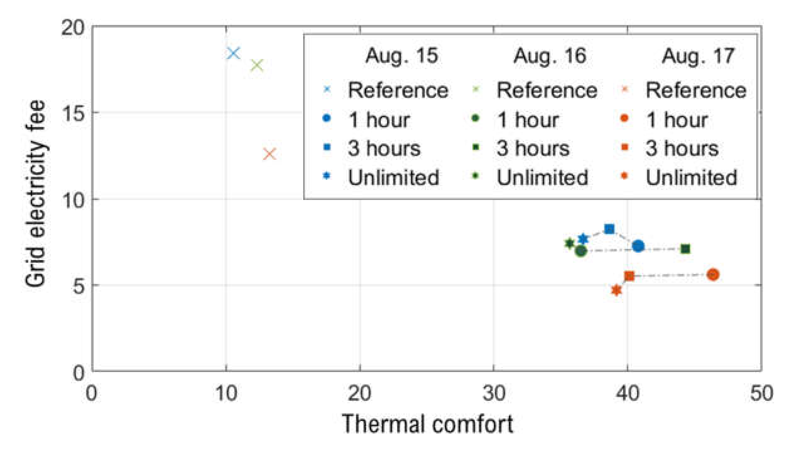
| Day | Cases | Grid Power Usage (kW) | Grid Electricity Price ($) | Saving Cost Rate (%) | CPU Time (min) | |
|---|---|---|---|---|---|---|
| 15 August | Reference | 114.6 | 18.4 | - | 10.5 | - |
| Opt. 1 h | 113.5 | 7.2 | 60.5 | 40.7 | 60 | |
| Opt. 3 h | 129.4 | 8.2 | 55.3 | 38.6 | 180 | |
| Opt. Inf | 114.9 | 7.6 | 58.3 | 36.6 | 485 | |
| 16 August | Reference | 110.3 | 17.7 | - | 12.3 | - |
| Opt. 1 h | 111.5 | 6.9 | 60.5 | 36.5 | 60 | |
| Opt. 3 h | 116.2 | 7.1 | 59.8 | 44.3 | 180 | |
| Opt. Inf | 14.3 | .4 | 58.1 | 35.6 | 556 | |
| 17 August | Reference | 7.3 | 2.6 | - | 13.2 | - |
| Opt. 1 h | 0.5 | 5.6 | 55.5 | 46.3 | 60 | |
| Opt. 3 h | 1.4 | 7.0 | 56.1 | 40.1 | 180 | |
| Opt. Inf | 91.2 | 4.7 | 62.6 | 39.1 | 501 |
Publisher’s Note: MDPI stays neutral with regard to jurisdictional claims in published maps and institutional affiliations. |
© 2022 by the authors. Licensee MDPI, Basel, Switzerland. This article is an open access article distributed under the terms and conditions of the Creative Commons Attribution (CC BY) license (https://creativecommons.org/licenses/by/4.0/).
Share and Cite
Jeon, B.-K.; Kim, E.-J. White-Model Predictive Control for Balancing Energy Savings and Thermal Comfort. Energies 2022, 15, 2345. https://doi.org/10.3390/en15072345
Jeon B-K, Kim E-J. White-Model Predictive Control for Balancing Energy Savings and Thermal Comfort. Energies. 2022; 15(7):2345. https://doi.org/10.3390/en15072345
Chicago/Turabian StyleJeon, Byung-Ki, and Eui-Jong Kim. 2022. "White-Model Predictive Control for Balancing Energy Savings and Thermal Comfort" Energies 15, no. 7: 2345. https://doi.org/10.3390/en15072345
APA StyleJeon, B.-K., & Kim, E.-J. (2022). White-Model Predictive Control for Balancing Energy Savings and Thermal Comfort. Energies, 15(7), 2345. https://doi.org/10.3390/en15072345