
Classification of Electronic Components Based on Convolutional Neural Network Architecture


Abstract
:1. Introduction
- -
- A new CNN model is proposed for classification studies.
- -
- The performance of the proposed model is not complicated by the pre-trained deep learning model.
- -
- The proposed model is fast and reliable and shows high performance.
- -
- There are less learner parameters of the proposed CNN model than those of other models, namely, AlexNet, ShuffleNet, SqueezeNet, and ResNet, which shortens the analysis time. Time saving is very significant, particularly when working with very large datasets.
2. Materials and Methods
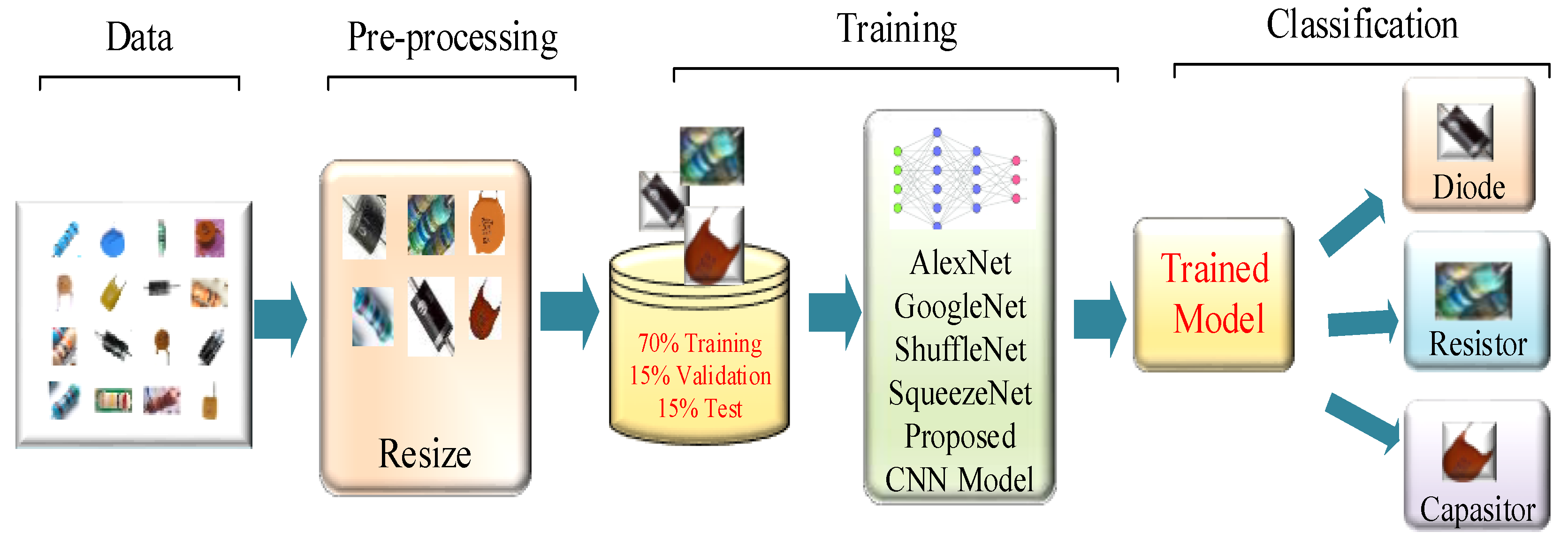
2.1. Proposed Deep Forecasting Method
2.2. Preprocessing and Data Augmentation
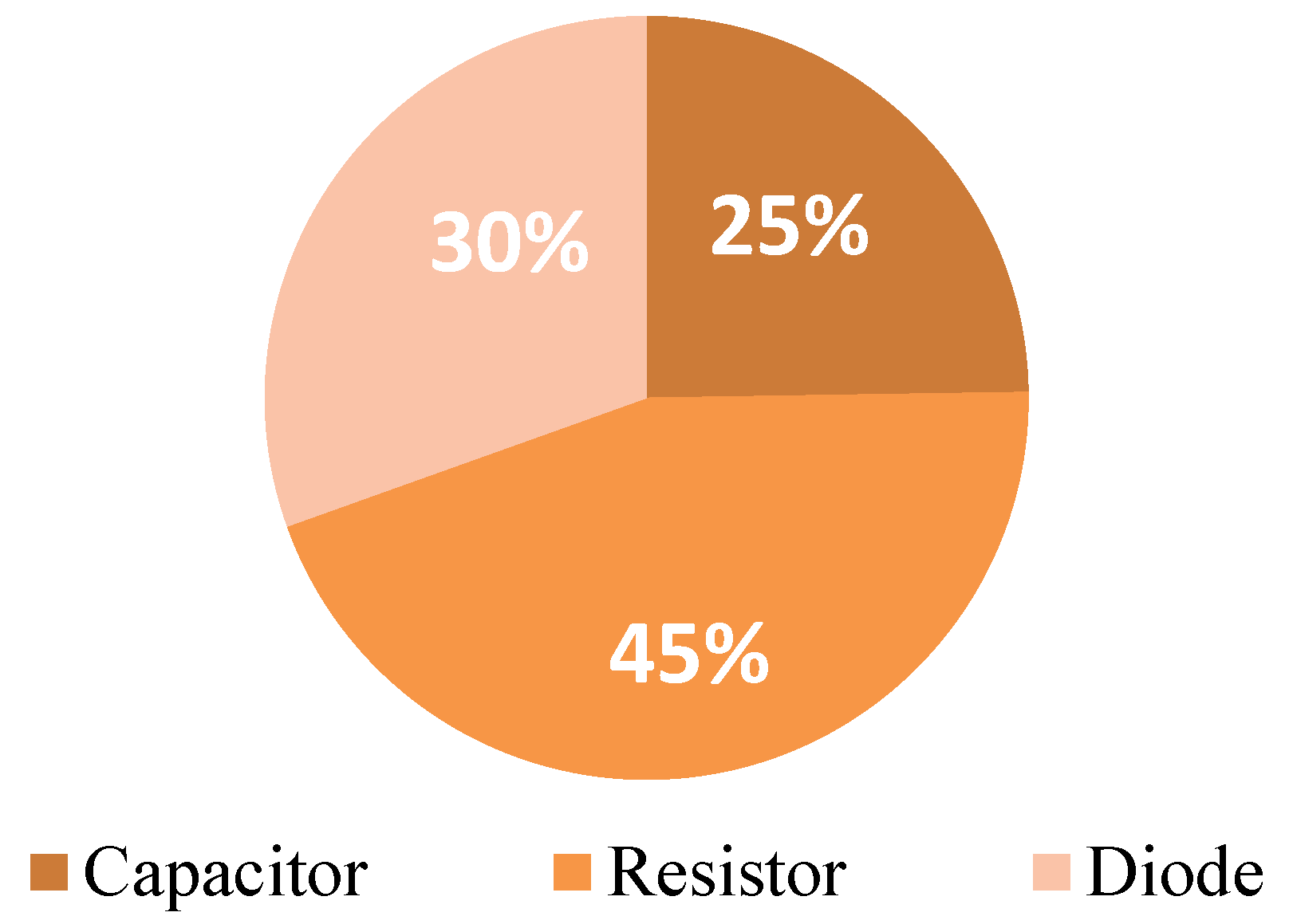
2.3. Dataset
2.4. Convolutional Neural Networks (CNNs)
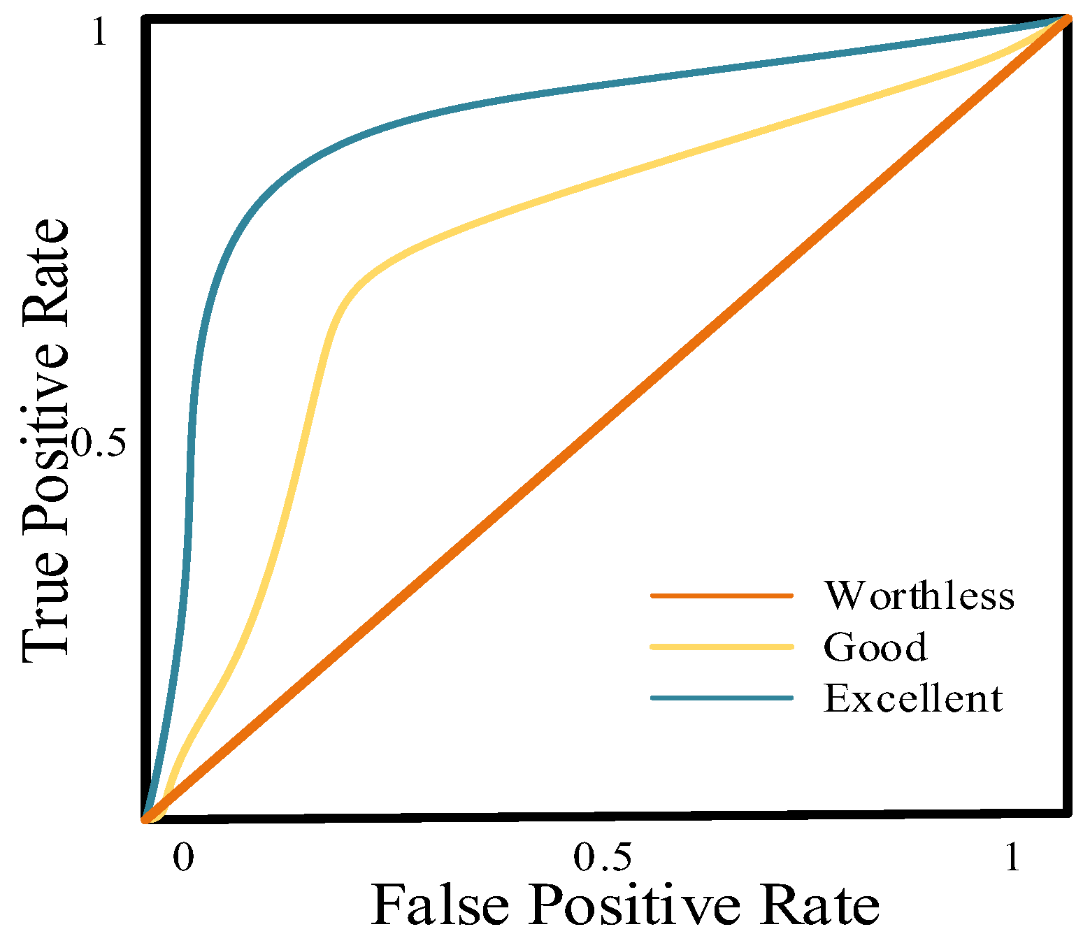
2.5. Performance Metrics
2.6. Pre-Trained CNN Models
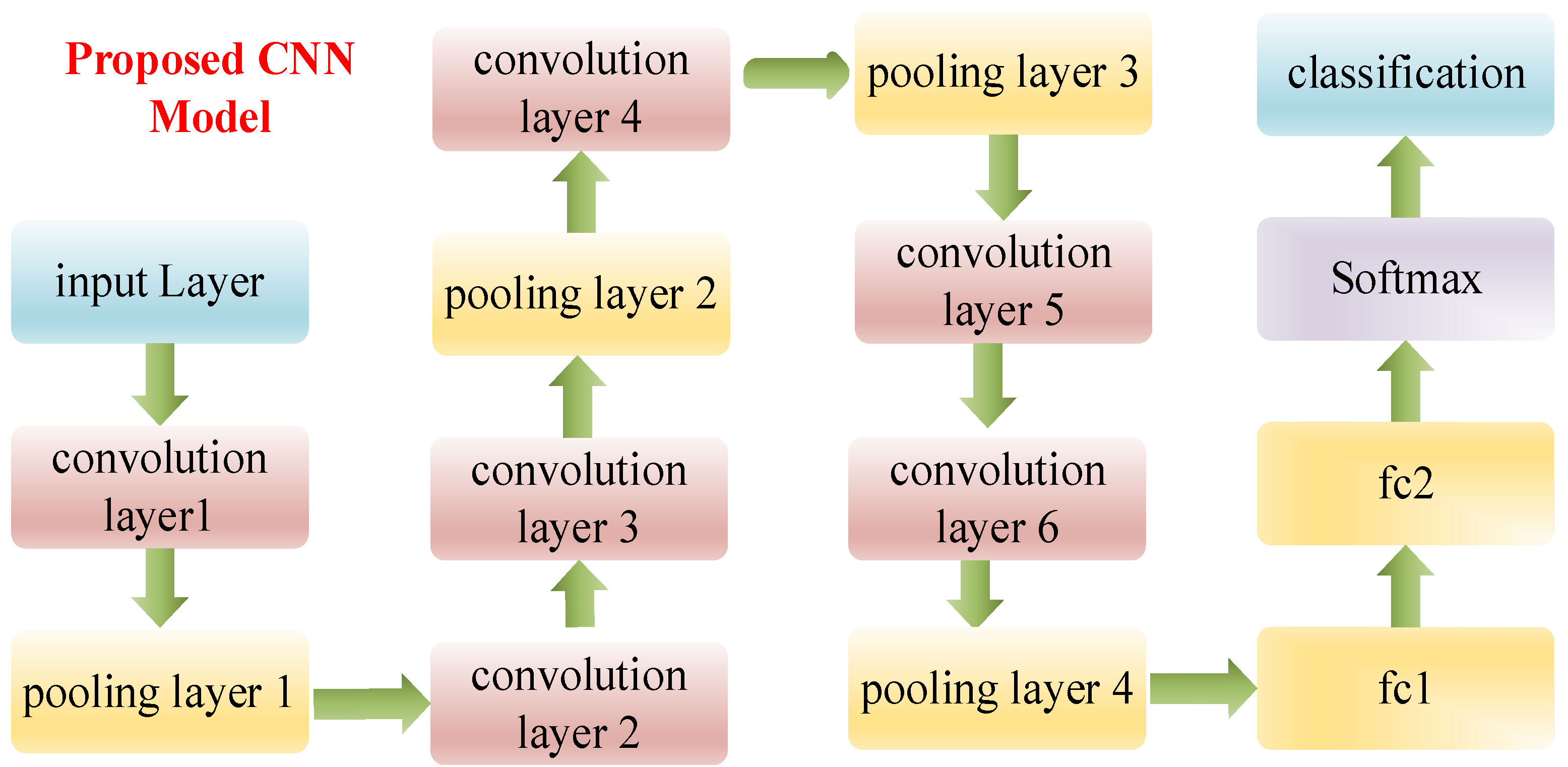
2.7. The Proposed CNN Model
3. Results
4. Discussion
5. Conclusions
Funding
Institutional Review Board Statement
Informed Consent Statement
Data Availability Statement
Conflicts of Interest
References
- Yuan, J.; Hou, X.; Xiao, Y.; Cao, D.; Guan, W.; Nie, L. Multi-criteria active deep learning for image classification. Knowl.-Based Syst. 2019, 172, 86–94. [Google Scholar] [CrossRef]
- Cetinic, E.; Lipic, T.; Grgic, S. Fine-tuning Convolutional Neural Networks for fine art classification. Expert Syst. Appl. 2018, 114, 107–118. [Google Scholar] [CrossRef]
- dos Santos, M.M.; da S. Filho, A.G.; dos Santos, W.P. Deep convolutional extreme learning machines: Filters combination and error model validation. Neurocomputing 2019, 329, 359–369. [Google Scholar] [CrossRef]
- Liang, Z. Automatic Image Recognition of Rapid Malaria Emergency Diagnosis: A Deep Neural Network Approach. Master’s Thesis, York University, Toronto, ON, Canada, 2017. Available online: https://yorkspace.library.yorku.ca/xmlui/handle/10315/34319 (accessed on 10 January 2022).
- Han, H.; Li, Y.; Zhu, X. Convolutional neural network learning for generic data classification. Inf. Sci. 2019, 477, 448–465. [Google Scholar] [CrossRef]
- Krizhevsky, A.; Hinton, G. Convolutional deep belief networks on cifar-10. Unpubl. Manuscr. 2010, 40, 1–9. Available online: https://www.cs.toronto.edu/~kriz/conv-cifar10-aug2010.pdf (accessed on 10 January 2022).
- Rasekh, M.; Karami, H.; Wilson, A.D.; Gancarz, M. Performance Analysis of MAU-9 Electronic-Nose MOS Sensor Array Components and ANN Classification Methods for Discrimination of Herb and Fruit Essential Oils. Chemosensors 2021, 9, 243. [Google Scholar] [CrossRef]
- Roy, S.S.; Rodrigues, N.; Taguchi, Y.-H. Incremental Dilations Using CNN for Brain Tumor Classification. Appl. Sci. 2020, 10, 4915. [Google Scholar] [CrossRef]
- Chapelle, O.; Haffner, P.; Vapnik, V.N. Support vector machines for histogram-based image classification. IEEE Trans. Neural Netw. 1999, 10, 1055–1064. [Google Scholar] [CrossRef]
- Marée, R.; Geurts, P.; Piater, J.; Wehenkel, L. A generic approach for image classification based on decision tree ensembles and local sub-windows. In Proceedings of the 6th Asian Conference on Computer Vision, Jeju, Korea, 27–30 January 2004; pp. 860–865. Available online: https://www.semanticscholar.org/paper/A-generic-approach-for-image-classification-based-Mar%C3%A9e-Geurts/134bb1cfe1cd0d37ef1cf091105a4e5a37241898 (accessed on 24 February 2022).
- Milgram, J.; Sabourin, R.; Cheriet, M. Combining model-based and discriminative approaches in a modular two-stage classification system: Application to isolated handwritten digit recognition. In Progress in Computer Vision and Image Analysis; World Scientific, 2010; pp. 181–205. Available online: https://dl.acm.org/doi/10.1145/2598394.2602287 (accessed on 5 December 2021).
- Zhong, Z.; Zheng, L.; Kang, G.; Li, S.; Yang, Y. Random Erasing Data Augmentation. In Proceedings of the AAAI Conference on Artificial Intelligence, New York, NY, USA, 7–12 February 2020; Volume 34, pp. 13001–13008. [Google Scholar]
- David, O.E.; Greental, I. Genetic algorithms for evolving deep neural networks. In Proceedings of the Companion Publication of the 2014 Annual Conference on Genetic and Evolutionary Computation, Vancouver, BC, Canada, 12–16 July 2014; pp. 1451–1452. [Google Scholar]
- Jia, Y.; Shelhamer, E.; Donahue, J.; Karayev, S.; Long, J.; Girshick, R.; Guadarrama, S.; Darrell, T. Caffe: Convolutional Architecture for Fast Feature Embedding. In Proceedings of the 22nd ACM International Conference on Multimedia, Orlando, FL, USA, 3–7 November 2014; pp. 675–678. [Google Scholar]
- Suganuma, M.; Shirakawa, S.; Nagao, T. A genetic programming approach to designing convolutional neural network architectures. In Proceedings of the Genetic and Evolutionary Computation Conference, Berlin, Germany, 15–19 July 2017; pp. 497–504. [Google Scholar]
- Bosch, A.; Zisserman, A.; Munoz, X. Image Classification using Random Forests and Ferns. In Proceedings of the 2007 IEEE 11th International Conference on Computer Vision, Rio de Janeiro, Brazil, 14–21 October 2007; pp. 1–8. [Google Scholar]
- Krizhevsky, A.; Sutskever, I.; Hinton, G.E. Imagenet classification with deep convolutional neural networks. Adv. Neural Inf. Process. Syst. 2012, 60, 84–90. [Google Scholar] [CrossRef]
- Ciresan, D.C.; Meier, U.; Masci, J.; Gambardella, L.M.; Schmidhuber, J. Flexible, high performance convolutional neural networks for image classification. In Proceedings of the Twenty-Second International Joint Conference on Artificial Intelligence, Barcelona, Spain, 16–22 July 2011. [Google Scholar]
- McDonnell, M.D.; Vladusich, T. Enhanced image classification with a fast-learning shallow convolutional neural network. In Proceedings of the 2015 International Joint Conference on Neural Networks (IJCNN), Killarney, Ireland, 12–17 July 2015; pp. 1–7. [Google Scholar]
- Springenberg, J.T.; Dosovitskiy, A.; Brox, T.; Riedmiller, M. Striving for simplicity: The all convolutional net. arXiv 2014, arXiv:1412.6806. [Google Scholar]
- Ronao, C.A.; Cho, S.-B. Human activity recognition with smartphone sensors using deep learning neural networks. Expert Syst. Appl. 2016, 59, 235–244. [Google Scholar] [CrossRef]
- Xiao, H.; Rasul, K.; Vollgraf, R. Fashion-mnist: A novel image dataset for benchmarking machine learning algorithms. arXiv 2017, arXiv:1708.07747. [Google Scholar]
- Kaggle. “Kaggle”. Kaggle Data Set. 6 December 2021. Available online: https://www.kaggle.com/datasets (accessed on 10 December 2021).
- Van Dyk, D.A.; Meng, X.-L. The Art of Data Augmentation. J. Comput. Graph. Stat. 2001, 10, 1–50. [Google Scholar] [CrossRef]
- Acikgoz, H. A novel approach based on integration of convolutional neural networks and deep feature selection for short-term solar radiation forecasting. Appl. Energy 2022, 305, 117912. [Google Scholar] [CrossRef]
- Atik, I. A New CNN-Based Method for Short-Term Forecasting of Electrical Energy Consumption in the Covid-19 Period: The Case of Turkey. IEEE Access 2022, 10, 22586–22598. [Google Scholar] [CrossRef]
- Park, Y.; Yang, H.S. Convolutional neural network based on an extreme learning machine for image classification. Neurocomputing 2019, 339, 66–76. [Google Scholar] [CrossRef]
- Hiary, H.; Saadeh, H.; Saadeh, M.; Yaqub, M. Flower classification using deep convolutional neural networks. IET Comput. Vis. 2018, 12, 855–862. [Google Scholar] [CrossRef]
- Samui, P.; Roy, S.S.; Balas, V.E. Handbook of Neural Computation; Academic Press: London, UK, 2017. [Google Scholar]
- Hoo, Z.H.; Candlish, J.; Teare, D. What is an ROC curve? Emerg. Med. J. 2017, 34, 357–359. [Google Scholar] [CrossRef]
- Ucar, F.; Korkmaz, D. COVIDiagnosis-Net: Deep Bayes-SqueezeNet based diagnosis of the coronavirus disease 2019 (COVID-19) from X-ray images. Med. Hypotheses 2020, 140, 109761. [Google Scholar] [CrossRef]
- Narayanan, B.N.; Ali, R.A.; Hardie, R.C. Performance analysis of machine learning and deep learning architectures for malaria detection on cell images. In Proceedings of the Applications of Machine Learning, San Diego, CA, USA, 11–15 August 2019; Volume 11139, p. 111390W. [Google Scholar]
- Agarap, A.F. Deep Learning using Rectified Linear Units (ReLU). arXiv 2018, arXiv:1803.08375. [Google Scholar]
- Sun, W.; Tseng, T.-L.; Zhang, J.; Qian, W. Enhancing deep convolutional neural network scheme for breast cancer diagnosis with unlabeled data. Comput. Med. Imaging Graph. 2017, 57, 4–9. [Google Scholar] [CrossRef] [Green Version]
- Pan, W.D.; Dong, Y.; Wu, D. Classification of Malaria-Infected Cells Using Deep Convolutional Neural Networks. Mach. Learn. Adv. Tech. Emerg. Appl. 2018, 159. [Google Scholar] [CrossRef] [Green Version]


| Author | Method | Dataset | Accuracy | Error Rate |
|---|---|---|---|---|
| Chapelle et al. [9] | - SVM | Corel7 Corel14 | 16.3% 11.0% | |
| Marée et al. [10] | - Decision tree community - Local sub-windows | MNIST ORL COIL-100 OUTEX | 3.26% 2.63% | |
| Milgram et al. [11] | - Hyperplanes-SVM | MNIST | 1.50% | |
| Zhong et al. [12] | - CNN - Random delete | Fashion-MNIST CIFAR-10 CIFAR-100 | 4.05% 3.08% 17.73% | |
| David and Greental [13] | - Genetic algorithm | MNIST | 1.44% | |
| Jia et al. [14] | - CNN | Caffe lib. CIFAR-10 | ||
| Suganuma et al. [15] | - CNN - Residual network | CIFAR-10 | 6.75% 5.98% | |
| Bosch et al. [16] | - Random forest algorithm - Fern algorithm | Caltech-101 | 80.0% 79.0% | |
| Krizhevsky [17] | - Deep Belief Network | CIFAR-10 CIFAR-100 | 79.0% | |
| Cireşan et al. [18] | - CNN | MNIST CIFAR-10 | 0.23% 11.21% | |
| McDonnell and Vladusich [19] | - Residual network | MNIST | 0.37% | |
| Springenberg et al. [20] | - CNN | CIFAR-10 CIFAR-100 | 4.41% 33.71% | |
| Ronao and Cho [21] | - CNN | Data obtained with the help of smartphone sensors | 96.7% | |
| Xiao et al. [22] | - SVC | Fashion-MNIST | 89.7% |
| Metric | Equation | Description |
|---|---|---|
| Accuracy | The accuracy rate is the ratio of the number of correctly classified samples to the total number of samples. | |
| Sensitivity | The number of correctly classified positive samples is the ratio of the total number of positive samples. | |
| Precision | Precision is the ratio of the number of true positive samples predicted as class 1 to the total number of samples predicted as class 1. | |
| F-Score | The harmonic mean of precision and sensitivity. |
| CNN | Image Input Size | Description |
|---|---|---|
| AlexNet | 227 × 227 | AlexNet has different levels of visual perception and is a high-performance CNN structure in image recognition. This architecture consists of 5 convolution layers, 3 pooling layers, and 3 full connection layers. |
| GoogleNet | 224 × 224 | GoogleNet architecture includes modules that come to the fore by reducing the cost of hCNN by making connections called Inception in its internal network. It consists of 144 layers. |
| SqueezeNet | 224 × 224 | The most basic feature of this architecture is that it can successfully analyze by reducing the size capacity and the number of parameters. |
| ShuffleNet | 224 × 224. | ShuffleNet has lower complexity and fewer parameters compared to other CNN architectures. |
| Layer | Input Size | Filter | Stride | Filter |
|---|---|---|---|---|
| convolution-1 | 227 × 227 | 3 × 3 | 1 | 8 |
| pooling-1 | 112 × 112 | 2 × 2 | 2 | 8 |
| convolution-2 | 56 × 56 | 5 × 5 | 1 | 8 |
| convolution-3 | 50 × 50 | 5 × 5 | 2 | 16 |
| pooling-2 | 44 × 44 | 2 × 2 | 1 | 16 |
| convolution-4 | 22 × 22 | 9 × 9 | 1 | 16 |
| pooling-3 | 6 × 6 | 2 × 2 | 2 | 32 |
| convolution-5 | 11 × 11 | 9 × 9 | 1 | 32 |
| convolution-6 | 11 × 11 | 9 × 9 | 1 | 64 |
| pooling-4 | 6 × 6 | 2 × 2 | 2 | 64 |
| Parameters | Value |
|---|---|
| Mini ensemble size | 16 |
| Maximum period | 100 |
| Initial learning rate | 1 × 10⁻³ |
| Optimize method | sgdm |
| Model | Accuracy (%) | Specificity | Sensibility | Precision | F-Score |
|---|---|---|---|---|---|
| AlexNet | 95.42 | 0.960 | 0.947 | 0.949 | 0.947 |
| GoogleNet | 96.67 | 0.964 | 0.970 | 0.964 | 0.966 |
| ShuffleNet | 92.95 | 0.919 | 0.938 | 0.924 | 0.930 |
| SqueezeNet | 93.86 | 0.926 | 0.949 | 0.930 | 0.939 |
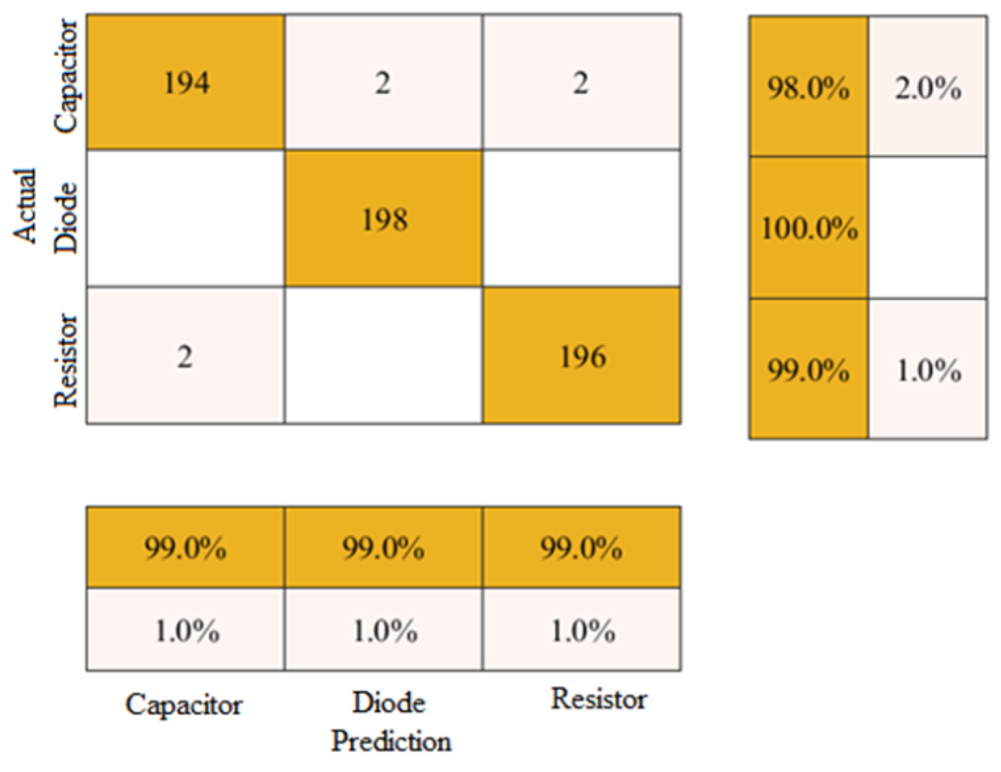
| Proposed CNN model | 98.99 | 0.976 | 0.986 | 0.988 | 0.987 |
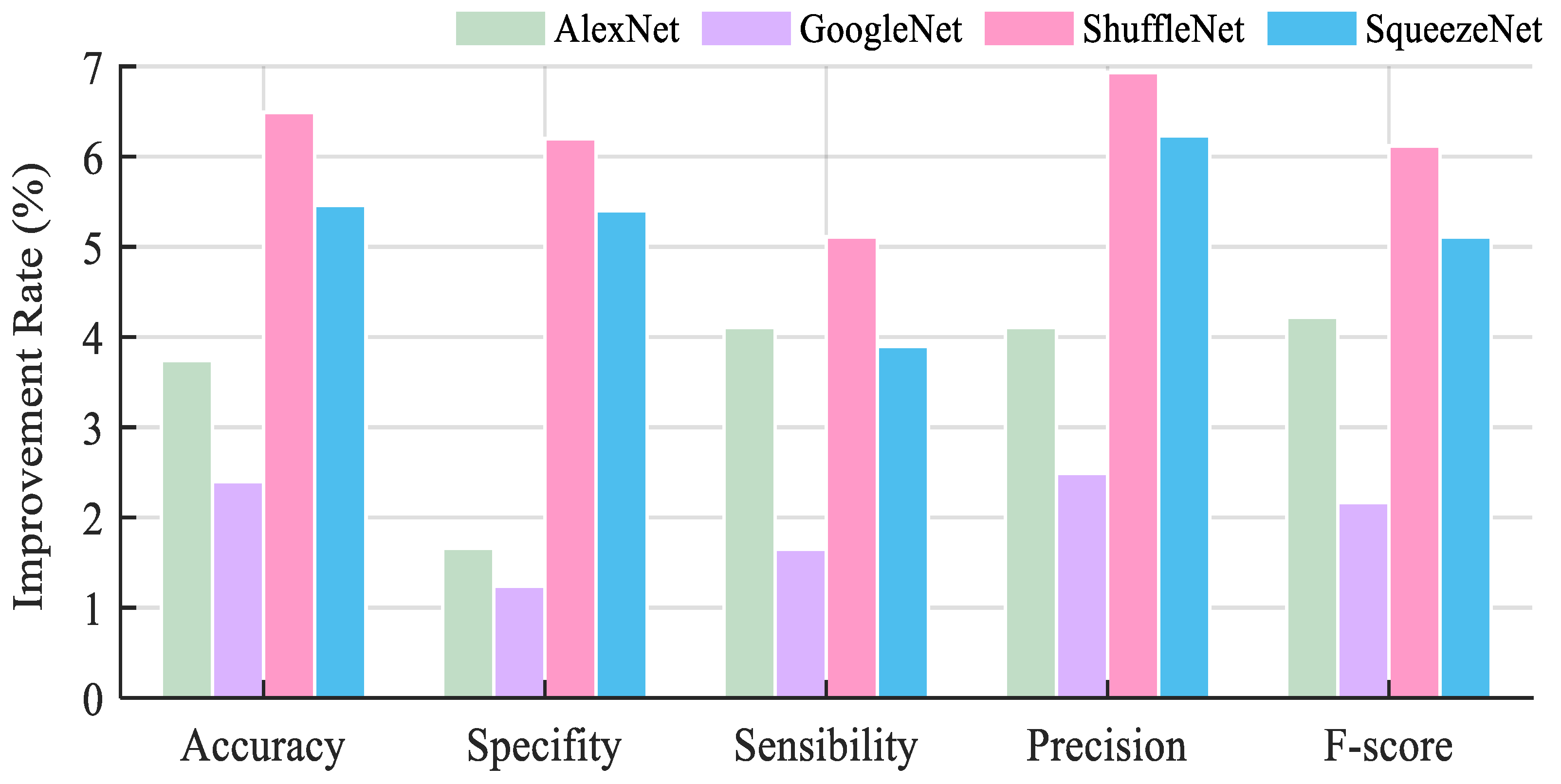
| Model | Accuracy (%) | Specificity | Sensibility | Precision | F-Score |
|---|---|---|---|---|---|
| AlexNet | 3.74% | 1.66% | 4.11% | 4.11% | 4.22% |
| GoogleNet | 2.40% | 1.24% | 1.65% | 2.49% | 2.17% |
| ShuffleNet | 6.49% | 6.2% | 5.11% | 6.93% | 6.12% |
| SqueezeNet | 5.46% | 5.4% | 3.9% | 6.23% | 5.11% |
| Reference | Method | Dataset | Accuracy Rate (%) |
|---|---|---|---|
| Agarap (2019) [33] | Feed forwad + CNN | MNIST | 97.98% |
| Fashion MNIST | 89.35% | ||
| Sun et. Al. (2017) [34] | Graph-based semi-supervised CNN | 1874 çift göğüs resmi | 82.43% |
| Ronao and cho (2016) [21] | CNN | Smartphone sensor data human activity recognation | 95.75% |
| LeNet-5 [35] | LeNET-5 | Malaria-infected cells dataset | %95 |
| Proposed CNN Model | CNN | Electronic components | 98.99% |
Publisher’s Note: MDPI stays neutral with regard to jurisdictional claims in published maps and institutional affiliations. |
© 2022 by the author. Licensee MDPI, Basel, Switzerland. This article is an open access article distributed under the terms and conditions of the Creative Commons Attribution (CC BY) license (https://creativecommons.org/licenses/by/4.0/).
Share and Cite
Atik, I. Classification of Electronic Components Based on Convolutional Neural Network Architecture. Energies 2022, 15, 2347. https://doi.org/10.3390/en15072347
Atik I. Classification of Electronic Components Based on Convolutional Neural Network Architecture. Energies. 2022; 15(7):2347. https://doi.org/10.3390/en15072347
Chicago/Turabian StyleAtik, Ipek. 2022. "Classification of Electronic Components Based on Convolutional Neural Network Architecture" Energies 15, no. 7: 2347. https://doi.org/10.3390/en15072347
APA StyleAtik, I. (2022). Classification of Electronic Components Based on Convolutional Neural Network Architecture. Energies, 15(7), 2347. https://doi.org/10.3390/en15072347