
IoT-Based PV Array Fault Detection and Classification Using Embedded Supervised Learning Methods


Abstract
:1. Introduction
- Investigation, discussion, emulation, simulation, classification, and implementation of a combination of important physical and environmental faults that affect PV modules;
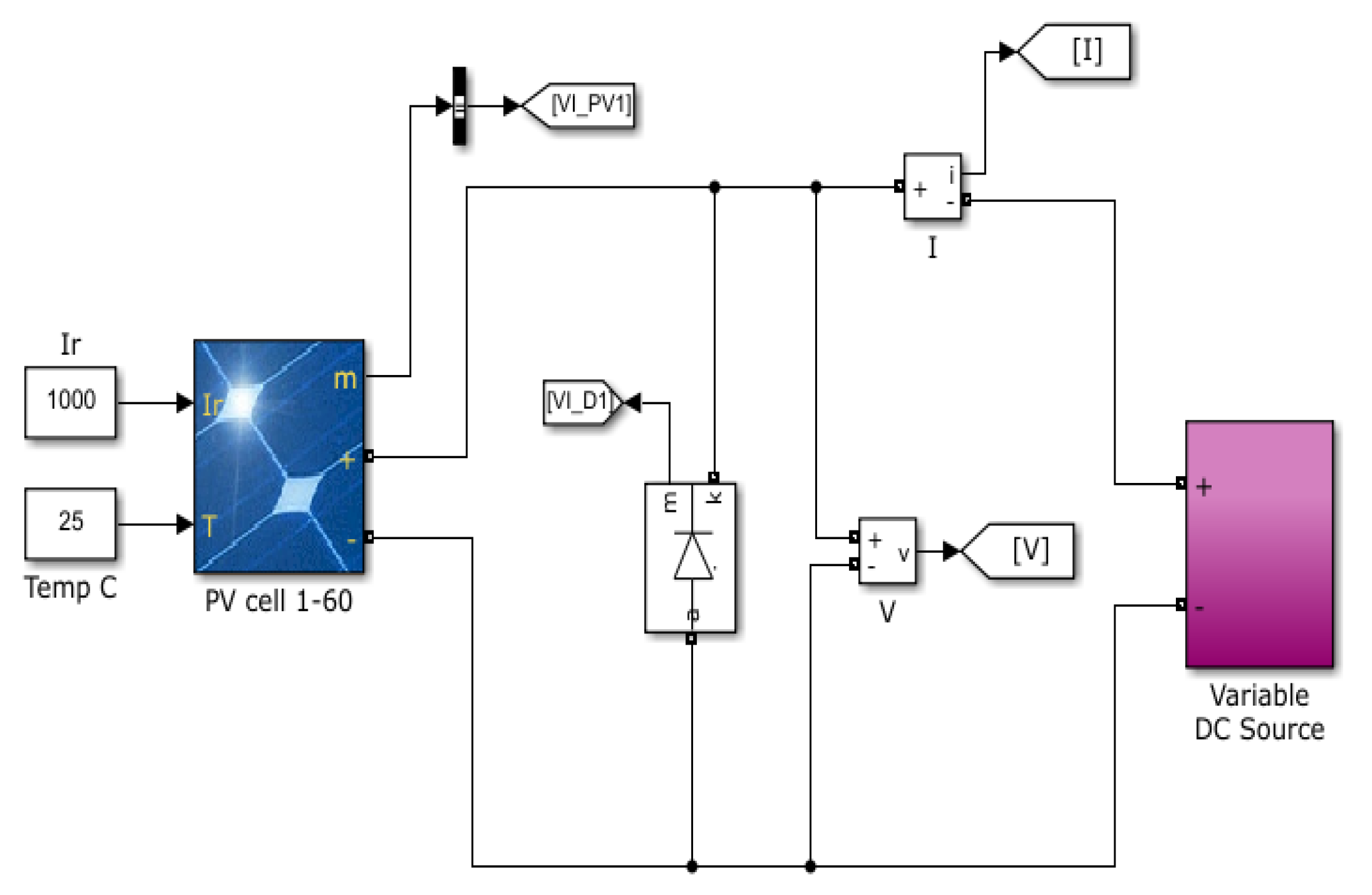
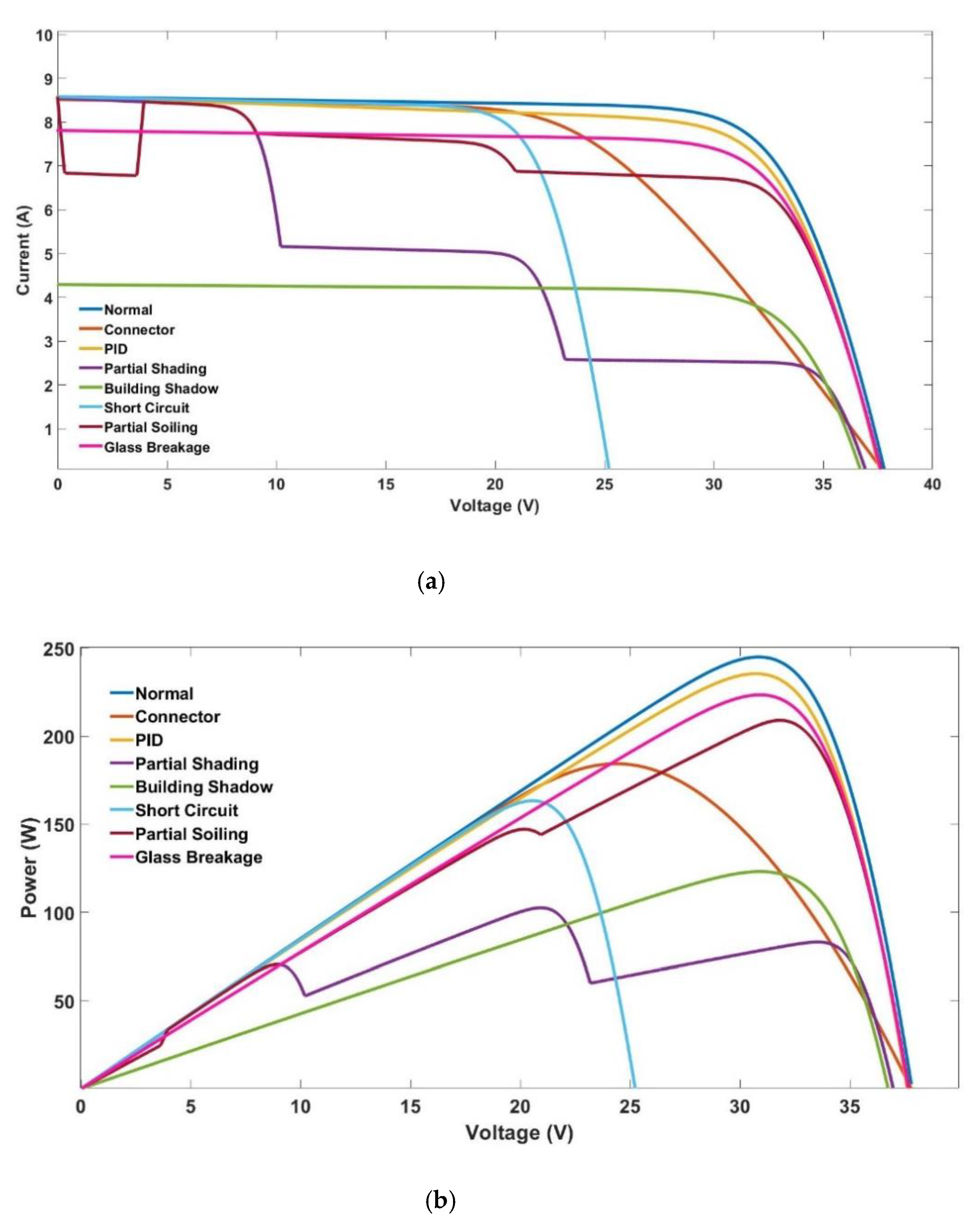
- Identification of the main features for module-level classification by analyzing the variations of the I-V and P-V characteristics of PV modules under normal and fault events using a Simulink-based model and literature review;
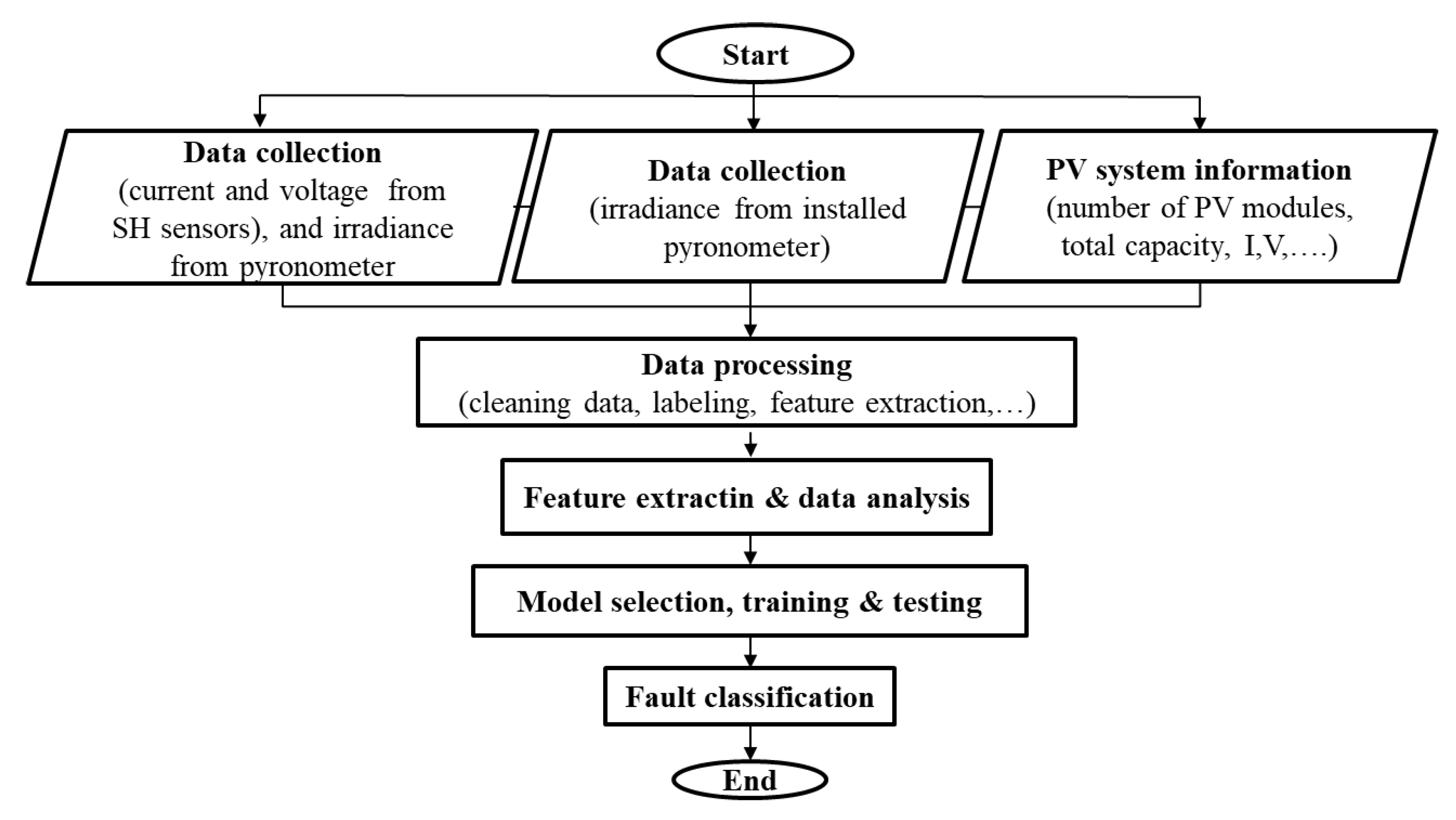
- Development of a PV fault detection process at the level of the PV module at the edge using ML techniques, based on measured data;
- Training, evaluation, and comparison of several supervised learning algorithms to define the best one to use for the edge computation of PV fault detection;
- Completion of a comparative study to further demonstrate the superiority of the proposed method for the detection and classification of faults;
- Selection of the best-performing algorithm to test on the real PV system.
2. PV Module Fault Definition and Simulation Approach
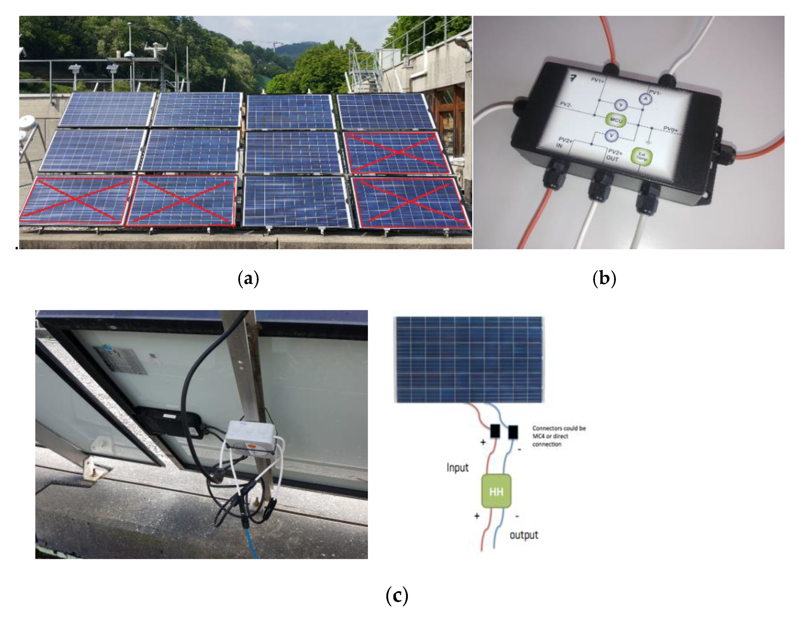
3. Experimental Setup
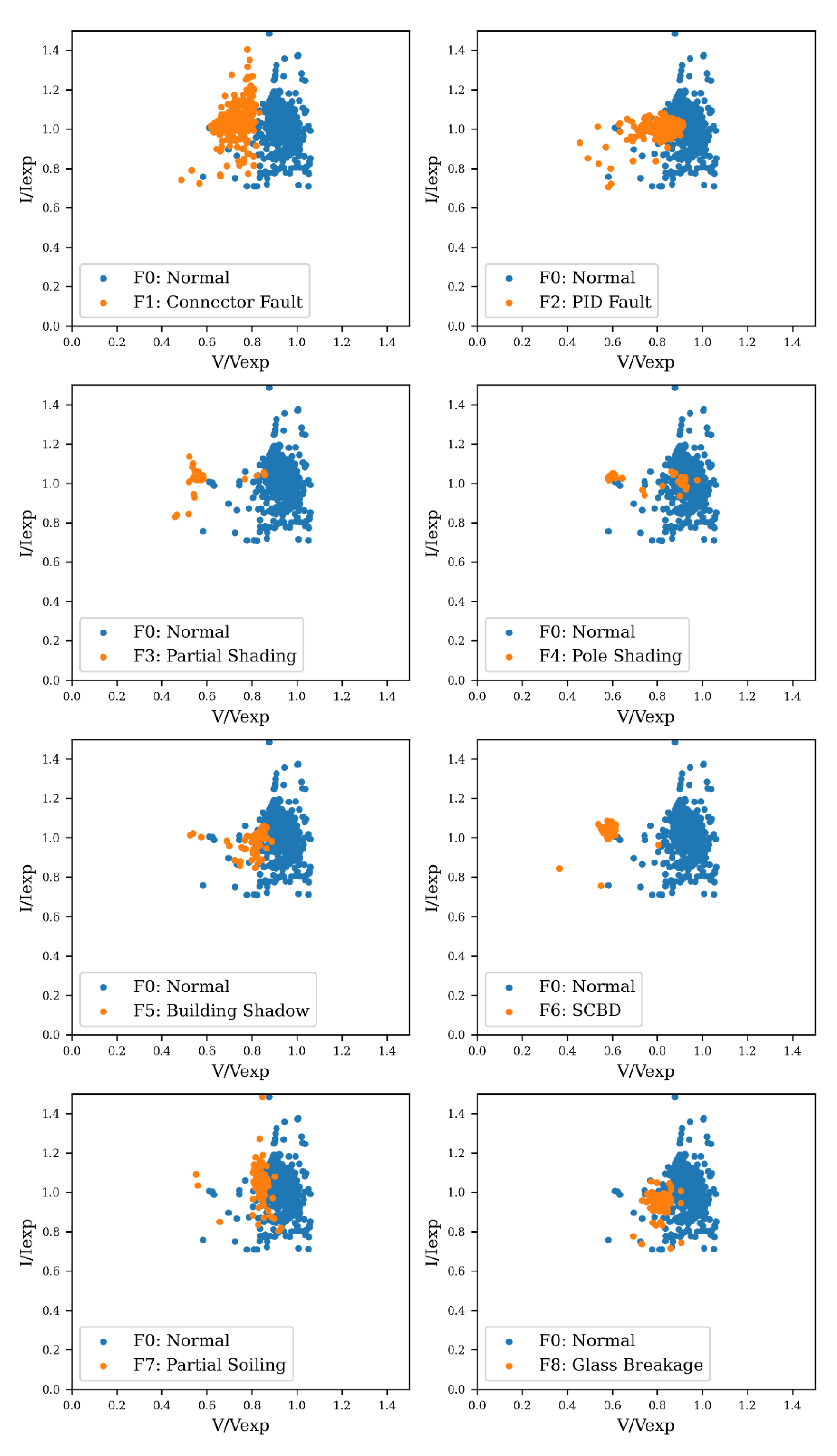
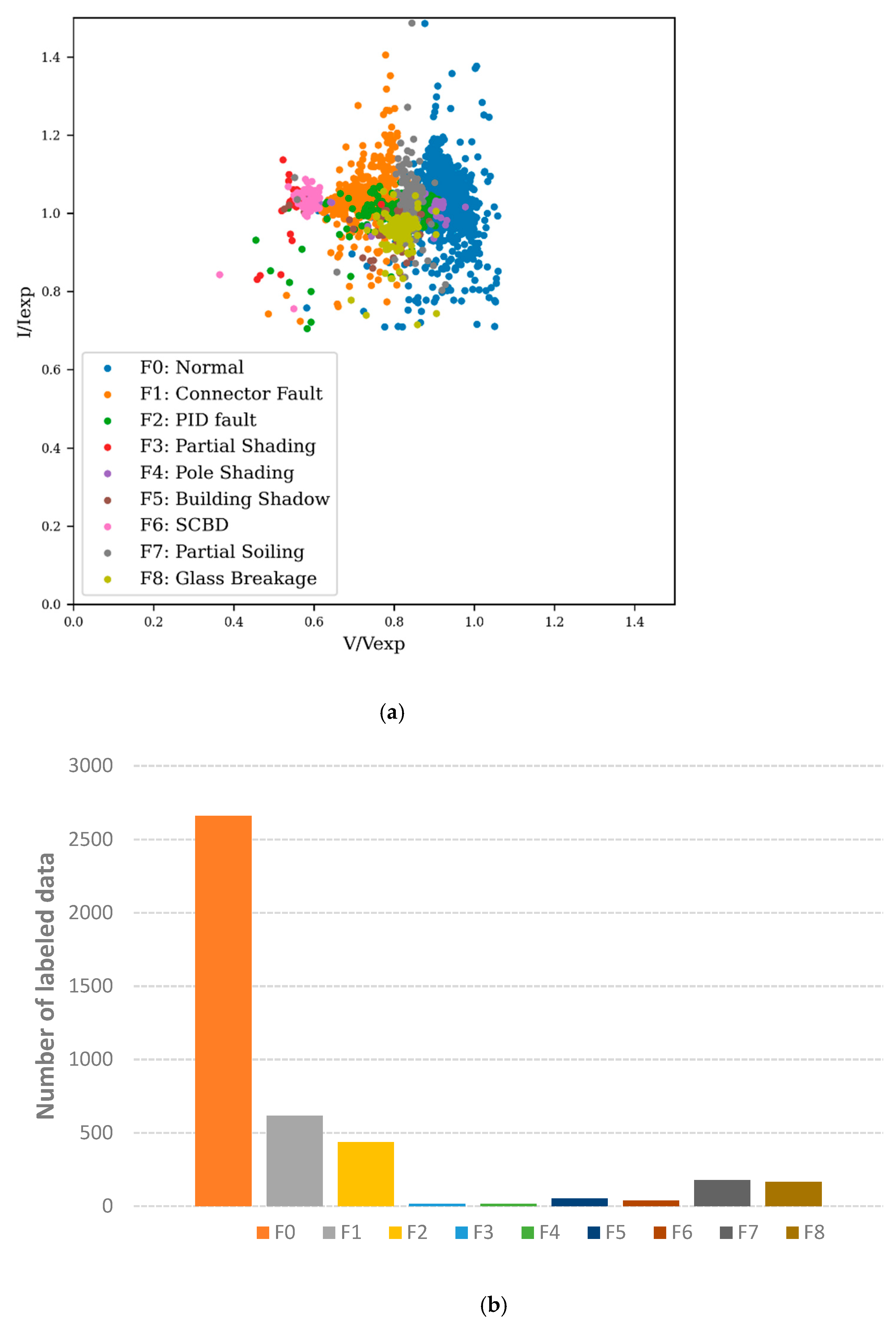
4. Feature Extraction and Data Analysis
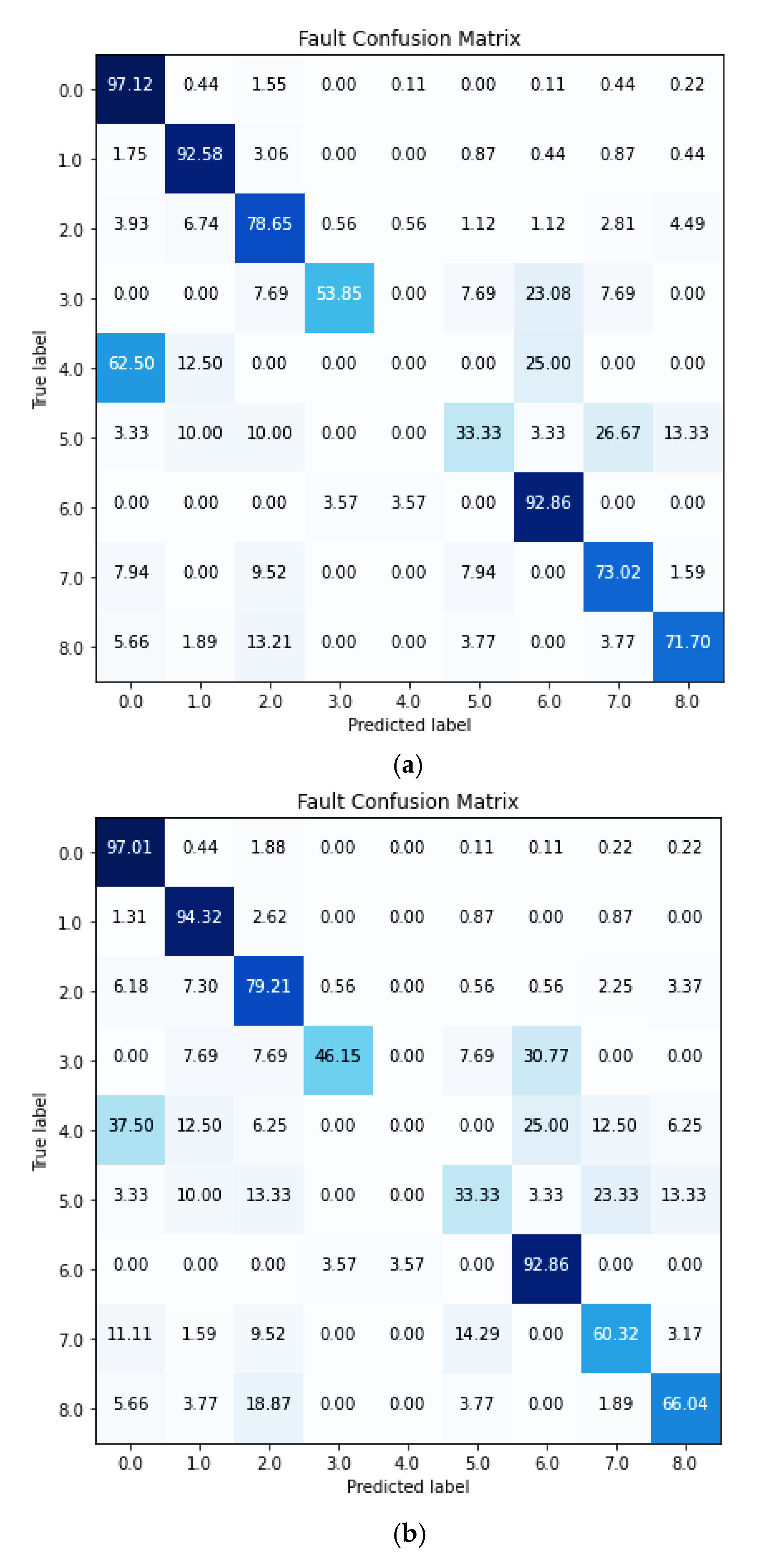
5. Fault Detection and Classification
6. Conclusions
Author Contributions
Funding
Acknowledgments
Conflicts of Interest
References
- Samkria, R. Automatic PV grid fault detection system with IoT and LabVIEW as data logger. Comput. Mater. Contin. 2021, 69, 1709–1723. [Google Scholar] [CrossRef]
- Fonseca Alves, R.H.; Deus Júnior, G.A.; Marra, E.G.; Lemos, R.P. Automatic fault classification in photovoltaic modules using convolutional neural networks. Renew. Energy 2021, 179, 502–516. [Google Scholar] [CrossRef]
- Djalab, A.; Rezaoui, M.M.; Mazouz, L.; Teta, A.; Sabri, N. Robust method for diagnosis and detection of faults in photovoltaic systems using artificial neural networks. Period. Polytech. Electr. Eng. Comput. Sci. 2020, 64, 291–302. [Google Scholar] [CrossRef]
- Sun, Y.; Wang, J.; Yang, Q.; Li, X.; Yan, W. Fault Diagnosis of Photovoltaic Module Based on Extreme Learning Machine Technique. In Proceedings of the IMCIC 2018—9th International Multi-Conference on Complexity, Informatics and Cybernetics, Proceedings, Orlando, FL, USA, 13–16 March 2018; Volume 1, pp. 34–39. [Google Scholar]
- Eskandari, A.; Milimonfared, J.; Aghaei, M. Fault detection and classification for photovoltaic systems based on hierarchical classification and machine learning technique. IEEE Trans. Ind. Electron. 2021, 68, 12750–12759. [Google Scholar] [CrossRef]
- Nieto, A.E.; Ruiz, F.; Patino, D.; Ramirez, O. Classification of electric faults in photovoltaic systems based on voltage-power curves. IEEE Lat. Am. Trans. 2021, 19, 2071–2078. [Google Scholar] [CrossRef]
- Zhao, Y.; Lehman, B.; Ball, R.; Mosesian, J.; De Palma, J.F. Outlier Detection Rules for Fault Detection in Solar Photovoltaic Arrays. In Proceedings of the Conference Proceedings—IEEE Applied Power Electronics Conference and Exposition—APEC, Long Beach, CA, USA, 17–21 March 2013. [Google Scholar] [CrossRef]
- Zaki, S.A.; Zhu, H.; Yao, J. Fault Detection and Diagnosis of Photovoltaic System Using Fuzzy Logic Control. E3S Web Conf. 2019, 107, 02001. [Google Scholar] [CrossRef]
- Mehmood, A.; Sher, H.A.; Murtaza, A.F.; Al-Haddad, K. A diode-based fault detection, classification, and localization method for photovoltaic array. IEEE Trans. Instrum. Meas. 2021, 70, 20987470. [Google Scholar] [CrossRef]
- Mehmood, A.; Sher, H.A.; Murtaza, A.F.; Al-Haddad, K. Fault detection, classification and localization algorithm for photovoltaic array. IEEE Trans. Energy Convers. 2021, 36, 2945–2955. [Google Scholar] [CrossRef]
- Chine, W.; Mellit, A.; Lughi, V.; Malek, A.; Sulligoi, G.; Massi Pavan, A. A novel fault diagnosis technique for photovoltaic systems based on artificial neural networks. Renew. Energy 2016, 90, 501–512. [Google Scholar] [CrossRef]
- Quiroz, J.E.; Stein, J.S.; Carmignani, C.K.; Gillispie, K. In-Situ Module-Level I-V Tracers for Novel PV Monitoring. In Proceedings of the 2015 IEEE 42nd Photovoltaic Specialist Conference, PVSC 2015, New Orleans, LA, USA, 15–19 June 2015. [Google Scholar] [CrossRef]
- Khelil, C.K.; Kara, K.; Chouder, A. Fault detection of the photovoltaic System by artificial neural networks. In Proceedings of the 4th International Conference on Green Energy and Environmental Engineering (GEEE-2017), Sousse, Tunisia, 22–24 April 2017. [Google Scholar]
- Dhimish, M.; Holmes, V.; Mehrdadi, B.; Dales, M.; Mather, P. Photovoltaic fault detection algorithm based on theoretical curves modelling and fuzzy classification system. Energy 2017, 140, 276–290. [Google Scholar] [CrossRef]
- Natarajan, K.; Kumar, B.P.; Kumar, V.S. Fault detection of solar PV system using SVM and thermal image processing. Int. J. Renew. Energy Res. 2020, 10, 967–977. [Google Scholar]
- Segovia Ramírez, I.; Das, B.; García Márquez, F.P. Fault detection and diagnosis in photovoltaic panels by radiometric sensors embedded in unmanned aerial vehicles. Prog. Photovolt. Res. Appl. 2022, 30, 240–256. [Google Scholar] [CrossRef]
- Jaskie, K.; Martin, J.; Spanias, A. PV fault detection using positive unlabeled learning. Appl. Sci. 2021, 11, 5599. [Google Scholar] [CrossRef]
- Bommes, L.; Pickel, T.; Buerhop-Lutz, C.; Hauch, J.; Brabec, C.; Peters, I.M. Computer vision tool for detection, mapping, and fault classification of photovoltaics modules in aerial IR videos. Prog. Photovolt. Res. Appl. 2021, 29, 1236–1251. [Google Scholar] [CrossRef]
- Dhimish, M.; Holmes, V.; Mehrdadi, B.; Dales, M. Comparing mamdani sugeno fuzzy logic and RBF ANN network for PV fault detection. Renew. Energy 2018, 117, 257–274. [Google Scholar] [CrossRef] [Green Version]
- Bharath Kurukuru, V.S.; Haque, A.; Khan, M.A. Fault Classification for Photovoltaic Modules Using Thermography and Image. In Proceedings of the 2019 IEEE Industry Applications Society Annual Meeting, IAS 2019, Baltimore, MD, USA, 29 September–3 October 2019. [Google Scholar] [CrossRef]
- Chen, L.C. Fault Diagnosis and Classification for Photovoltaic Arrays Based on Principal Component Analysis and Support Vector Machine. IOP Conf. Ser. Earth Environ. Sci. 2018, 188, 012089. [Google Scholar] [CrossRef]
- Aghaei, M.; Fairbrother, A.; Gok, A.; Ahmad, S.; Kazim, S.; Lobato, K.; Oreski, G.; Reinders, A.; Schmitz, J.; Theelen, M.; et al. Review of degradation and failure phenomena in photovoltaic modules. Renew. Sustain. Energy Rev. 2022, 159, 112160. [Google Scholar] [CrossRef]
- SUPSI. SMARTHELIO Innosuisse Check Project; Final Report; Innosuisse: Bern, Switzerland, 2020. [Google Scholar]
- Sapountzoglou, N.; Raison, B.A. Grid Connected PV System Fault Diagnosis Method. In Proceedings of the 20th IEEE International Conference on Industrial Technology, Melbourne, Australia, 13–15 February 2019; Available online: https://hal.archives-ouvertes.fr/hal-02072272 (accessed on 30 January 2022).
- Machine Learning in Python. Available online: https://scikit-learn.org/stable/ (accessed on 30 January 2022).
- TensorFlow. Available online: https://www.tensorflow.org/resources/learn-ml?gclid=Cj0KCQiA09eQBhCxARIsAAYRiymFz-0aitHhd4ubbmbJjW_Ot-YMhiVmzudEVggGw6CR7r9kbWKG2rcaAsSYEALw_wcB (accessed on 30 January 2022).
- Morales, J.L.; Nocedal, J. Remark on Algorithm 778: L-BFGS-B: Fortran subroutines for large-scale bound constrained optimization. ACM Trans. Math. Softw. 2011, 38, 2–5. [Google Scholar] [CrossRef]
- Sridharan, N.V.; Sugumaran, V. Convolutional neural network based automatic detection of visible faults in a photovoltaic module. Energy Sources Part A Recovery Util. Environ. Eff. 2021, 1–16. [Google Scholar] [CrossRef]


| Ref. | Method | Technology | Faults | Classification Accuracy |
|---|---|---|---|---|
| [15] | SVM | Thermal image | Cell crack, soiling, and hot spot caused by shading conditions | 97 |
| [14] | Curve modeling & FUZZY | Thermal image | Different partial shading conditions | 98.8 |
| [3] | ANN | Electrical measurement (V, I, and P) in DC side | Connector fault, SC, bypass diode, and partial shading conditions | 94 |
| [2] | CNN | Thermal image | Bypass diode, hot spot, soiling, cell crack, and shading conditions | 92.5 |
| [13] | ANN | and from measurement & simulation | SC | NA |
| [8] | Fuzzy logic control (FLC) | Electrical measurement (V, I, and P) in DC side | SC, OC, and snow cover | NA |
| [18] | ResNet | Thermal IR video | SC, OC, hot spot, PID | 90 |
| [6] | V-P | Measuring and analyzing V-P in AC side | LL, LG, OC | 94.4 |
| [19] | Fuzzy logic and RBF ANN | Electrical measurement in DC side | Different partial shading conditions | 92.1 |
| [11] | ANN | Comparing simulation and electrical measurement in DC side | Partial shading conditions, connector fault | 90.3 |
| [20] | ANN, SVM, KNN | Thermal image | Faulty and normal conditions | 92.8 |
| [5] | Hierarchical classification | I-V characteristics of PV array | LL & LG | 96.66 |
| [7] | Outlier detection rules | String current | LL, OC, degradation, and partial shading condition | NA |
| [21] | SVM | Electrical measurement in DC side | SC, OC, partial shading condition | NA |
| [4] | RBF-kernel ELM | I-V curve tracing | SC, OC, degradation, and partial shading condition | NA |
| [17] | Feedback enhanced MLR (MLRf) | Electrical measurement in DC side | SC, soiling, partial shading condition | NA |
| [12] | Loss factors model (LFM) | I-V curve tracing | Partial shading condition, degradation | NA |
| [9,10] | Diode-based fault detection | Voltage measurement (array voltage, voltage at the positive node of the top and bottom module of a string) | LG, LL within a string, LL between two strings and partial shading condition | NA |
| PV Module Faults | ||
|---|---|---|
| Physical | Internal | EVA |
| External | connector | |
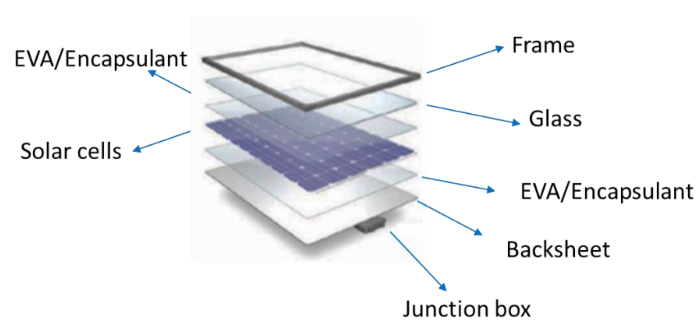
| glass breakage | ||
| cell crack | ||
| degradation/PID | ||
| Environmental | Temporary | dust accumulation |
| soiling | ||
| Permanent | hot spot | |
| Electrical | Internal | bypass diode faults |
| open circuit (OC) | ||
| External | line-line fault (LLF) | |
| arc fault | ||
| ground fault | ||
| Parameter | Value |
|---|---|
| 245 | |
| 8.58 | |
| 37.80 | |
| 7.94 | |
| 30.85 | |
| cells per module | 60 |
| temperature coefficient of | −0.34 |
| temperature coefficient of | 0.05 |
| Type of Fault | Label | Effects | ||||||||
|---|---|---|---|---|---|---|---|---|---|---|
| Isc | Voc | Imp | Vmp | Rs | Rsh | Np 3 | FF | Pmax | ||
| Connector fault (corrosion of cell connection) | F1 | ↓ 1 | ↓↓ | ↑ 2 | ↓↓ | ↑ | − | 1 | ↓↓ | ↓↓ |
| PID | F2 | ↓ | ↓ | ↓ | ↓ | − | ↓ | 1 | ↓ | ↓ |
| Partial shading condition | F3 | ↓ | − | ↓ | ↓ | − | − | >1 | ↓↓↓ | ↓↓↓ |
| Building shading condition | F5 | ↓↓↓ | ↓↓ | ↓↓↓ | ↓↓ | − | − | 1 | ↓↓↓ | ↓↓↓ |
| Failing bypass diode/ short circuit (SC) | F6 | − | ↓↓↓ | − | ↓↓↓ | − | − | 1 | ↓↓ | ↓↓ |
| Partial soiling | F7 | ↓ | − | ↓ | ↓↓↓ | − | − | >1 | ↓ | ↓ |
| Glass breakage | F8 | ↓↓ | − | ↓↓ | − | − | − | 1 | ↓ | ↓ |
| Symbol | Type of Fault | Fault Simulation | Fault Emulation |
|---|---|---|---|
| F1 | Connector | Connect 1 resistor in series with the module | Connect 1 resistor in series with the module |
| F2 | PID | Add 100 resistor in parallel with the PV module | Add 100 resistor in parallel with the PV module |
| F3 | Partial shading condition/bypass diode activation | Use 60% irradiance filter on 1/3 of the PV module and 30% irradiance filter on 1/3 of the PV module | Use foil to activate the bypass diode on the west string |
| F4 | Pole shading condition | − | Shading with pole on the east string |
| F5 | Building shadow condition | Add a 50% irradiance filter on two PV modules in one string | Shadow on two sub-strings in two PV modules |
| F6 | Short circuit bypass diode | Short circuit one bypass diode | Short circuit one bypass diode |
| F7 | Soiling | Use 90% irradiance filter on 1/3 of the module and 80% irradiance filter on 1/3 of the PV module |
|
| F8 | Glass breakage | Apply 91% irradiance filter | Place a foil with 91% transparency on the whole PV module |
| Classifier | Accuracy | Precision | Recall | F1 | Matthews Correlation Coefficient |
|---|---|---|---|---|---|
| Random Forest | 0.893 | 0.885 | 0.893 | 0.886 | 0.819 |
| Nearest Neighbors | 0.889 | 0.877 | 0.889 | 0.879 | 0.812 |
| Neural Net | 0.886 | 0.875 | 0.886 | 0.878 | 0.809 |
| Support Vector Machine | 0.883 | 0.866 | 0.883 | 0.871 | 0.799 |
| Decision Tree | 0.864 | 0.863 | 0.864 | 0.863 | 0.772 |
| Linear SVM | 0.858 | 0.851 | 0.858 | 0.832 | 0.758 |
| Logistic Regression | 0.744 | 0.586 | 0.744 | 0.649 | 0.527 |
| Classifier | Accuracy | Precision | Recall | F1 | Matthews Correlation Coefficient |
|---|---|---|---|---|---|
| Neural Net | 0.930 | 0.930 | 0.930 | 0.929 | 0.880 |
| Random Forest | 0.925 | 0.924 | 0.925 | 0.924 | 0.873 |
| Nearest Neighbors | 0.923 | 0.921 | 0.923 | 0.921 | 0.869 |
| Support Vector Machine | 0.917 | 0.918 | 0.917 | 0.915 | 0.860 |
| Decision Tree | 0.898 | 0.899 | 0.898 | 0.896 | 0.826 |
| Linear SVM | 0.892 | 0.895 | 0.892 | 0.878 | 0.816 |
| Logistic Regression | 0.767 | 0.644 | 0.767 | 0.691 | 0.573 |
Publisher’s Note: MDPI stays neutral with regard to jurisdictional claims in published maps and institutional affiliations. |
© 2022 by the authors. Licensee MDPI, Basel, Switzerland. This article is an open access article distributed under the terms and conditions of the Creative Commons Attribution (CC BY) license (https://creativecommons.org/licenses/by/4.0/).
Share and Cite
Hojabri, M.; Kellerhals, S.; Upadhyay, G.; Bowler, B. IoT-Based PV Array Fault Detection and Classification Using Embedded Supervised Learning Methods. Energies 2022, 15, 2097. https://doi.org/10.3390/en15062097
Hojabri M, Kellerhals S, Upadhyay G, Bowler B. IoT-Based PV Array Fault Detection and Classification Using Embedded Supervised Learning Methods. Energies. 2022; 15(6):2097. https://doi.org/10.3390/en15062097
Chicago/Turabian StyleHojabri, Mojgan, Samuel Kellerhals, Govinda Upadhyay, and Benjamin Bowler. 2022. "IoT-Based PV Array Fault Detection and Classification Using Embedded Supervised Learning Methods" Energies 15, no. 6: 2097. https://doi.org/10.3390/en15062097
APA StyleHojabri, M., Kellerhals, S., Upadhyay, G., & Bowler, B. (2022). IoT-Based PV Array Fault Detection and Classification Using Embedded Supervised Learning Methods. Energies, 15(6), 2097. https://doi.org/10.3390/en15062097