Article

Noise Reduction Study of Pressure Pulsation in Pumped Storage Units Based on Sparrow Optimization VMD Combined with SVD

1
School of Electric Power, North China University of Water Resources and Electric Power, Zhengzhou 450045, China
2
Energy and Power Engineering Institute, Zhengzhou Electric Power College, Zhengzhou 450000, China
3
China Nuclear Power Engineering Co., Ltd., Shenzhen 518124, China
4
State Grid Hunan Electric Power Co., Ltd., Changsha 410004, China
5
Hunan Heimifeng Pumped Storage Power Co., Ltd., State Grid Xin Yuan Company, Changsha 410213, China
*
Author to whom correspondence should be addressed.
Energies 2022, 15(6), 2073; https://doi.org/10.3390/en15062073
Submission received: 3 February 2022 / Revised: 2 March 2022 / Accepted: 10 March 2022 / Published: 11 March 2022

Abstract

:
The unbalanced forces generated by pumped storage units operating under non-ideal operating conditions can cause pressure pulsations. Due to the noise interference, the feature information reflecting the operating state of the unit in the pressure pulsation is difficult to extract. Therefore, this paper proposes a noise reduction method based on sparrow search algorithm (SSA) optimized variational mode decomposition (VMD) combined with singular value decomposition (SVD). Firstly, SSA is used to realize the adaptive optimization of VMD parameters for ideal decomposition of the signal. Then, the noise reduction of the decomposed signal is performed by using the sensitivity of the Permutation Entropy (PE) for small mutations. The noise reduction and reconstruction of the decomposed signal are carried out again by using SVD. The experimental and comparison results show that the mean square error of the signal after VMD-SVD feature extraction is reduced from 1.0068 to 0.0732 and the correlation coefficient is increased from 0.2428 to 0.9614. It is proved that the method achieves better results in the pressure pulsation signal of pumped storage units and has some application significance for the fault diagnosis of pumped storage units.

1. Introduction

Vibration in pumped storage units poses a significant threat to the safe and stable operation of the units [1,2]. Pumped storage units have the characteristics of rapid start-up and shutdown, peak cutting and valley filling, etc., which play an important supporting role in the construction of a new power system with new energy as the main body [3,4]. In order to smooth the new energy output, pumped storage units often deviate from the optimal operating conditions into the vibration zone when operating in new power systems. Pumped storage units operating in the vibration zone can cause strong draft tube pressure pulsations resulting in fatigue damage to the unit and affecting its performance [5]. The draft tube pressure pulsation signal is disturbed by ambient noise, the effective features are often masked by a large amount of noise, and the non-linearity and non-smoothness of the vibration signal is increasing. Noise reduction and feature extraction of draft tube pressure pulsations can increase unit operating efficiency and reduce economic losses [6].
A lot of research has been done on noise reduction and feature extraction of vibration signals [7,8,9]. Among them, short-time Fourier transform (STFT) [10,11], wavelet transform (WT) [12,13,14], empirical mode decomposition (EMD) [15,16], ensemble empirical mode decomposition (EEMD) [17,18], and other signal decomposition methods are more common. However, all of the above methods have certain limitations. STFT enables time-frequency analysis, but the fixed window function makes time-frequency analysis lack in adaptability. The WT makes use of the scalable nature of the wavelet basis functions to give good resolution, but some of the wavelet basis and threshold functions can cause unsatisfactory noise reduction results. EMD is achieved by time-scale transformation of the signal, which often results in mode mixing due to the uncertainty of the frequency and bandwidth of each mode during decomposition. The EEMD solves the mode mixing problem posed by EMD by adding random white noise to the original signal. However, the signal decomposition of EEMD is often accompanied by end effects that may cause signal deficiencies and affect the processing effect [19]. Based on the above analysis, it is important to propose a time-frequency signal processing method that is applicable to non-smooth non-linear signals. Singular value decomposition (SVD) is a noise reduction method based on phase space reconstruction, which achieves noise reduction by removing the reconstructed signal components corresponding to smaller singular values [20]. Reference [21] proposes an optimal wavelet demodulation method based on singular value decomposition (SVD), which can accurately detect the shock component in vibration signals. In [22], a combined adaptive local iterative filtering (ALIF) and SVD method was used for dual noise reduction and feature extraction of draft tube pressure pulsation, which was verified in simulation experiments and measured draft tube pressure pulsation data. Dragomiretskiy [23,24,25,26] proposed a variational mode decomposition (VMD) method based on non-recursive signals to achieve better results in the decomposition of vibration signals. Reference [27] used VMD to decompose the vibration signal, avoiding the mode mixing problem caused by EMD, and extracted a wealth of information on fault characteristics. Furthermore, [28] proposed a noise reduction method based on VMD and quantum particle swarm optimization adaptive stochastic resonance to achieve good noise reduction in early faint fault features. However, the effect of VMD decomposition is influenced by the iteration K and the penalty factor a. Too large a value of K or a can easily lead to over-decomposition of mode mixing; too small a value of K or a can easily lead to under-decomposition. Some of the literature is based on experience or observation to determine parameter combinations, which is subjective and random [29]. In recent years, some scholars have proposed to seek the optimal parameters of VMD by optimization algorithms. Traditional optimization algorithms [30,31,32] are well established but often fall into local optima when solving, making it difficult to achieve satisfactory results for the complexity of vibration signals. It is important to implement an adaptive decomposition of the VMD parameters using an algorithm with a strong global search capability.
Based on the above analysis, the SSA [33] has a flexible and efficient global search capability, with stronger convergence and better optimization accuracy and stability. Adaptive optimization of VMD parameters can be achieved using SSA. VMD and SVD have been applied to non-stationary vibration signals and have effectively avoided the problem of mode mixing in the decomposed signal, considering that the draft tube pressure pulsation contains a wealth of characteristic information about the unit’s operating conditions for the pressure pulsation characteristics of the draft tube of pumped storage units [34,35]. In this paper, we propose a study on pressure pulsation reduction of pumped storage units based on sparrow optimization VMD combined with SVD.
This paper takes pumped storage units as the research object, and the main contributions are as follows: (1) By comparing the computational cost of envelope entropy (EE), sample entropy (SE), and permutation entropy (PE), it is determined that the EE is used as the fitness function of the SSA to achieve adaptive optimization of the VMD parameters. (2) Using the EE as the fitness function, the SSA, the particle swarm optimization (PSO), and the genetic algorithm (GA) were compared in terms of their ability to find the optimal VMD parameters, and the SSA was determined as the optimization algorithm for the VMD parameters. (3) By comparing the noise reduction ability of different entropies, it was determined that PE would be used as the feature extraction method. (4) Calculate the PE after VMD decomposition and select the optimal PE parameter by comparing the entropy values under different embedding dimensions and delay time conditions. The signal components whose PE values are less than the set threshold are retained for reconstruction to achieve preliminary noise reduction of the noisy signal. (5) The signal after the initial noise reduction is noise reduced again by using SVD, and the effectiveness of various feature extraction methods is evaluated by using the correlation coefficient and mean square error as evaluation indexes.
The rest of the paper is as follows: Section 2 introduces the basic principles of the noise-carrying signal noise reduction method based on SSA optimization VMD combined with SVD and establishes the framework flow chart of the research method. Section 3 constructs a simulation signal based on the pressure pulsation characteristics of the draft tube of pumped storage units and determines the optimal parameters of the proposed method in this paper. Section 4 compares the proposed method with reported noise reduction methods using simulated signals and evaluation metrics to demonstrate the effectiveness of the method.

2. Methods

2.1. VMD

VMD is a new method for non-recursive signal decomposition proposed by Dragomiretskiy [36]. Constraints are used as the theoretical basis for constructing the overall framework and searching for variational modes by iteration. The decomposition of a signal consisting of multiple components into K intrinsic mode functions with fixed central frequencies ω k . The mode mixing problems are avoided and local features are highlighted for subsequent signal analysis.
(1)
Mode components u k   of the analytic signal
After Hilbert’s method calculation, each intrinsic mode function is considered as an FM-AM mode function.
  u k ( t ) = A k ( t ) cos ( k ( t ) )
where A k ( t ) is the instantaneous amplitude of u k ( t ) , k ( t ) is the instantaneous phase of   u k ( t ) . The derivative of the instantaneous phase with respect to time is the instantaneous frequency ω k ( t ) = d k ( t ) /dt.
(2)
Estimation of the frequency bandwidth of each intrinsic mode function
Using Hilbert’s transformation of the mode component u k ( t ) , one can obtain the one-sided spectral equation. Gaussian smoothing is used to obtain the bandwidth of the analytic signal after frequency shift, that is, the square root of the norm gradient L 2 . The variational problem is constructed as follows:
{ min { k = 1 k t ( δ ( t ) + j π t ) u k   ( t )   e j w k   ( t )   }   2 2     s .   t .   k = 1 k u k = f ( t )
where t is the partial derivative of the function with respect to time t,   δ ( t ) is the unit time impulse function,   e j w k   ( t ) is the correction exponent, and f ( t )   is the signal input function.
(3)
Introduction of the Lagrange quadratic constraint and solution using alternating operators
The unconstrained variational solution is established by augmenting Lagrange method as in Equation (3). After that, the alternating direction multiplier algorithm is used to continuously iteratively update the solution to obtain the generalized function as in Equation (4):
L ( { u k } , { ω k } , λ ) = a k   t [ ( δ ( t ) + j π t ) u k   ( t ) ] e j w k   ( t )   2 2 +   f ( t ) k u k ( t )   2 2   + < λ ( t ) , f ( t ) k   u k   ( t ) >  
where a is the penalty factor, and λ ( t ) is the Lagrangian multiplier.
u ^ k n + 1 = f ^ ( w ) i k   u ^ i n + 1 ( ω ) + λ ^     ( t ) 2   1 + 2 a ( ω ω k 2 ) ω k n + 1   = 0 ω | u ^ k ( ω )   |     2   d ω 0 | u ^ k ( ω )   |       2 d ω
(4)
Termination conditions
k = 1 k ( u ^ k n + 1 u ^ k n   2 2 / u ^ k n   2 2   ) < ε
The iteration ends when the constraint satisfies the above equation, otherwise a circular iteration is performed and a series of intrinsic mode functions are obtained at the end of the iteration.

2.2. Adaptive Optimization of VMD Parameters

2.2.1. SSA Principles

The SSA is a group intelligence optimization algorithm that simulates the foraging and anti-predatory act of sparrows. The algorithm is built by simulating the following acts: finders search for food while avoiding the danger of predation; joiners compete for food resources by monitoring the finders. Assume that the sparrow population size is N, the number of iterations is t, the dimensionality of the optimization variables is   d m i n , and the fitness is f .   The sparrow’s ability to search for food is strongest when the fitness is best.
Assuming that the finder searches for the widest range of food, the iterative process updates the finder’s location search as follows:
  X i , j t + 1 = { X i , j t   · exp ( i a · i t e r max ) i f   R 2 < S T   X i , j t + Q · L   i f   R 2 S T
where t is the number of iterations, i t e r max is the current maximum number of iterations, X i , j   is the position information of i-th sparrow in the j-th dimension, R 2 is the warning value, S T is the safety value, a is the random number of (0, 1], Q is a random number obeying normal distribution, and L denotes a 1 × d matrix. When R 2  < ST, it means there is no predator in the foraging environment, and the finder can continue searching. When R 2  ≥ ST, the predator appears and the sparrow needs to change the area to search.
Joiners compete for food resources with discoverers by monitoring their tracks, and a joiner’s location search is updated as follows:
  X i , j t + 1 = { Q · exp ( X worst X i , j t i 2   ) i f   i > n / 2 X p t + 1 + | X i , j t X p t + 1 | · A + · L     otherwise
where X p   is the optimal position of the current discoverer, X worst is the worst position currently searched, and A denotes a 1 × d matrix. When i > n / 2 , it means that the joiner cannot obtain food resources due to low adaptation.
The locations of some of the individual sparrows in the sparrow population that realized the approaching danger and made a zone change were updated as follows:
X i , j t + 1 = { X best t + β · | X i , j t X b e s t t | i f   f   i > f   g X i , j t + K · ( |   X i , j t X worst t   | ( f   i f w ) + ε ) i f     f   i = f   g
where X best   is the current global optimal position, f   i   is the i-th individual sparrow fitness, f   g   is the current global best fitness, f w is the current global worst fitness value, β is a random number obeying normal distribution, K is a random number of [−1, 1], and ε   is a constant.

2.2.2. VMD Parameter Optimization Based on SSA

The EE can measure the extent to which a signal contains fault information based on the sparsity of the signal. If the signal contains more noise, the signal is less sparse and has a higher EE. The signal X i has the following expression for the EE.
{ E p = i = 1 N p i lg   p i p i = a ( i ) / i = 1 N a ( i )  
where   E p is the signal X i of the EE, a ( i ) is the signal X i the envelope signal after Hilbert calculation, and p i is the normalized form of the   a ( i )   .    
Reference [37] used EE as a fitness function to optimize the VMD parameters in order to make the SSA process of optimizing the VMD parameters more accurate. Firstly, the VMD parameters are initialized, using the parameters [a, K] as particle positions. The EE is used as the fitness function to calculate the EE value of each particle under the VMD decomposition. The positions of sparrow discoverers, joiners, and other individuals are calculated according to Equations (6)–(8) for individual and global search. The particle positions are continuously updated and the combination of parameters with the smallest EE is recorded. When the number of iterations is satisfied, the loop is jumped out at the end of the iteration and the optimal parameter combination [a, K] is output.

2.3. PE

PE is an effective calculation method proposed by Christophet et al. to detect signal dynamic mutation and time series randomness [38]. PE can be used to filter the mode information and distinguish the noise dominant component from the effective signal component with rich feature information. The noise interference components with relatively high entropy values are removed by preset threshold for the purpose of denoising. The principle of the algorithm is as follows:
(1)
Suppose a time series X i and reconstruct its phase space; the matrix is obtained as follows:
  {   X 1 = { X 1 , X 1 + τ , , X 1 + ( m 1 ) τ , } X 2 = { X 2 , X 2 + τ , , X 2 + ( m 1 ) τ , } X r = { X r , X r + τ , X r + ( m 1 ) τ }
where m   is the embedding dimension and τ is the delay time. r is the number of row vectors to reconstruct.
(2)
Each row of the matrix is considered as a reconstructed component, and the elements are rearranged in ascending order to obtain:
  X i = { X ( i + ( ε 1 1 ) × τ ) } X ( i + ( ε 2 1 ) × τ ) X ( i + ( ε m 1 ) × τ )   }
where ε 1 , ε 2 , , ε m   is the column index of each element in the reconstructed component.
(3)
Calculate the probability of indexing P 1     , P 2 , P 3   at different positions. Define the normalized PE of the indexed series at different positions of the time series according to the form of entropy.
H = ( i = 1 r P i · lg p ) l g ( m ! )

2.4. SVD

SVD is a noise reduction method based on phase space reconstruction. As the noise signal has a different correlation to the original signal, by observing the singular value SVD spectrum, the singular value components representing the noise after decomposition are zeroed out and the singular values of the valid signal are retained [39]. Noise reduction of the characteristic matrix is achieved by the inverse of the SVD. For the signal   X i , the Hankel matrix is constructed as follows:
H = [ X ( 1 ) X ( q ) X ( d ) X ( N ) ]
The SVD decomposition of the H matrix is as follows:
  Q = U [   K 0 0 0 ] V T
where U, V are orthogonal matrices.   K = diag ( σ 1 , σ 2 , σ 3 ) forms the fault feature vector.
The PE value of the components after VMD decomposition is calculated, and the effective components smaller than the PE threshold are retained for reconstruction. The VMD-PE denoised signal is constructed as a Hankel matrix for SVD decomposition to achieve noise reduction again.

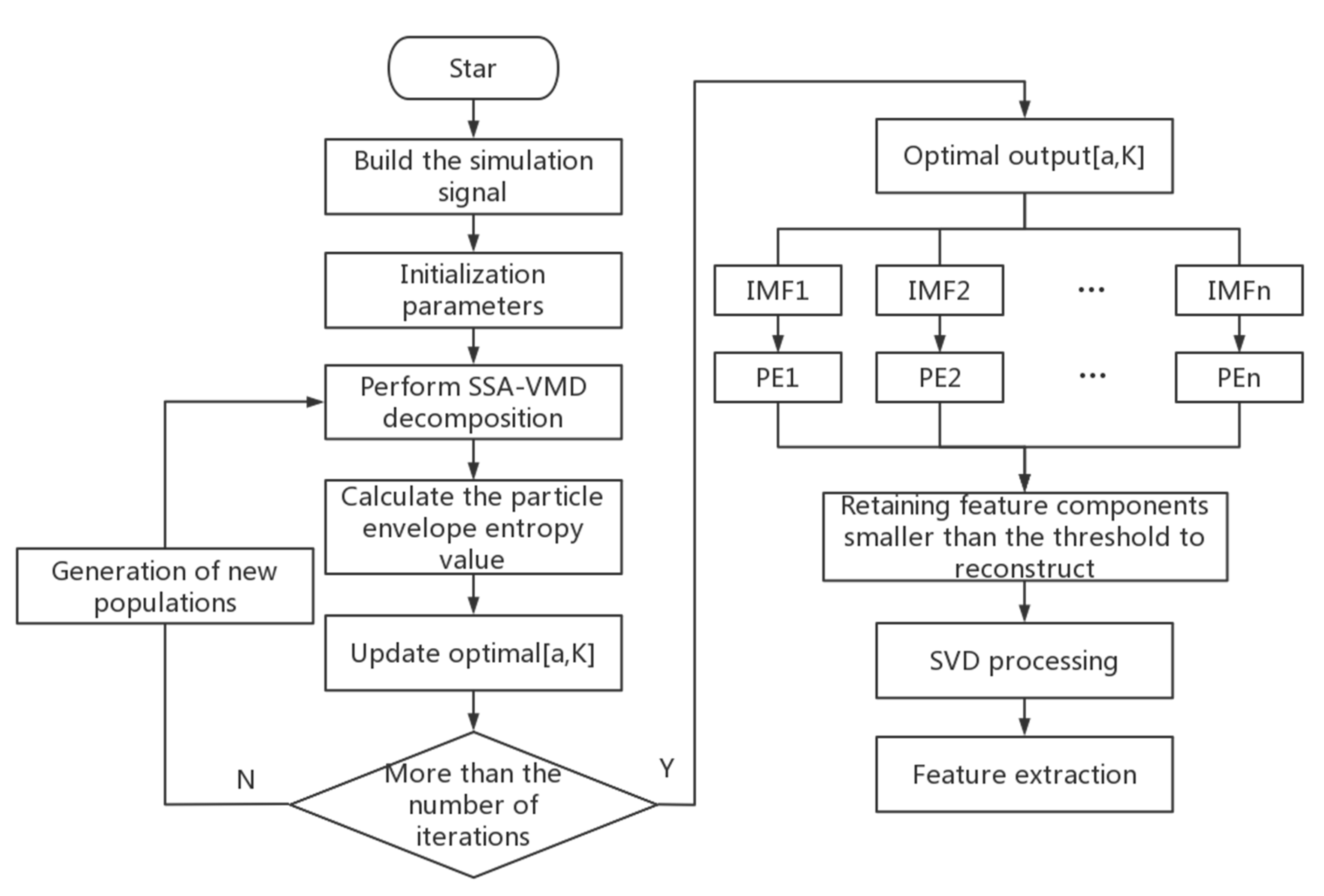
2.5. Noise Reduction Steps

Figure 1 shows the flow chart of the SSA–VMD–SVD framework, and the specific steps are shown below:
Step 1: Acquisition of vibration signals, setting the number of sampling points and sampling frequency.
Step 2: Determine the fitness function and establish an adaptive decomposition method for VMD parameters based on SSA, setting the population size to 10 and the maximum number of iterations to 20.
Step 3: Initialize the VMD parameters, using the parameters [a, K] as particle positions. The range of a is [1000, 3000] and the range of K is [2, 10]. The optimal combination of parameters with the smallest fitness function is obtained by SSA global search.
Step 4: Perform a VMD decomposition according to the optimal combination of parameters [a, K] to obtain K IMF components.
Step 5: Calculate the PE value of each component according to Equations (10)–(12) and set the PE threshold based on multiple simulations to achieve the initial noise reduction of the noisy signal.
Step 6: The initial noise reduction signal is decomposed by SVD according to Equation (14) to achieve the noise reduction of the reconstructed signal again.
Step 7: Extract the fault feature vector and perform a spectrum analysis to identify the cause of the fault.

3. Results

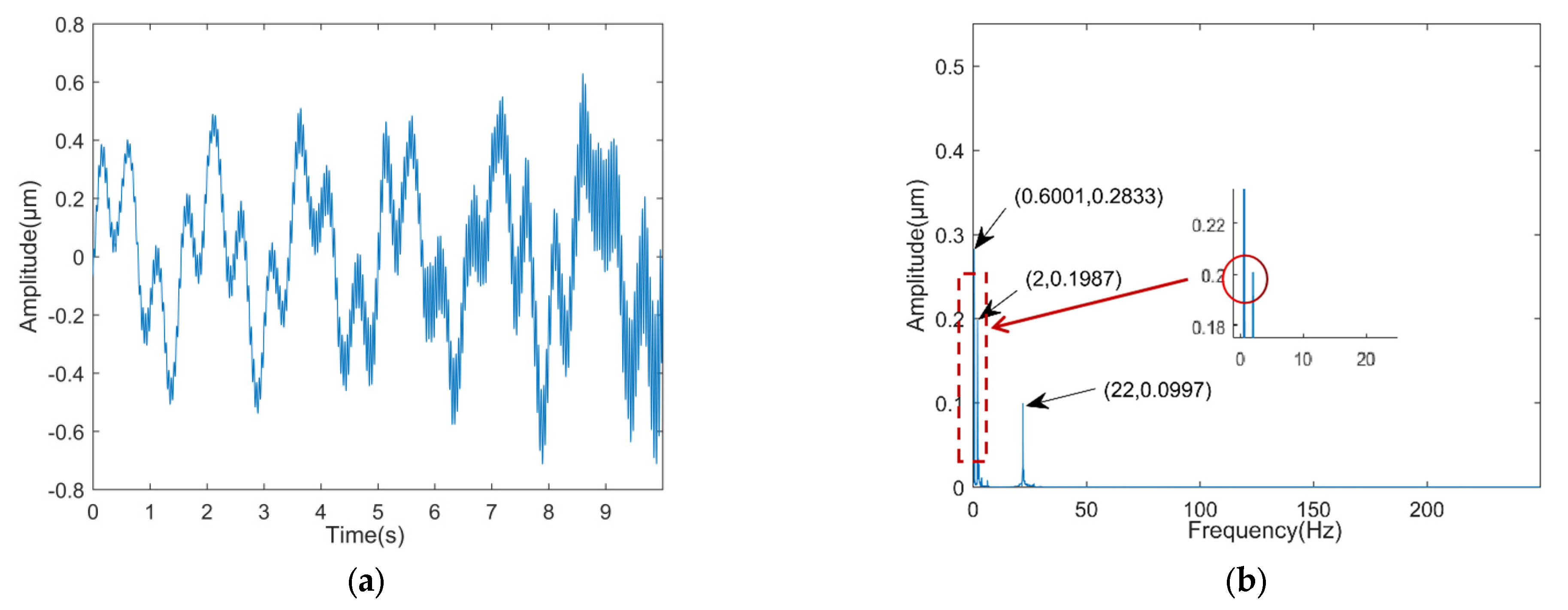
3.1. Simulation Signal

The main cause of the draft tube pressure pulsation is the low frequency vortex band, but there is also a certain amount of medium and high frequency pressure pulsation. The low-frequency pulsation frequency is about 0.15–0.30 times, and the medium-high frequency pressure pulsation frequency is close to the unit rotation frequency. In order to verify the effectiveness of the algorithm in extracting the pressure pulsation signal in the draft tube in this paper, the simulation signal A expression is established as follows:
    X 1 =     0.3 · sin ( 2 π t   f 1 ) + 0.2 · sin ( 2 π t   f 2 ) + 0.1 sin · ( 2 π t   f 3 ) X 2 = rand   ( 1 ,   5000 ) X t = X 1 + X 2
where f 1 is 0.6 Hz, f 2 is 2 Hz, and f 3 is 22 Hz; set the sampling frequency to 500 and the number of sampling points N to 5000.

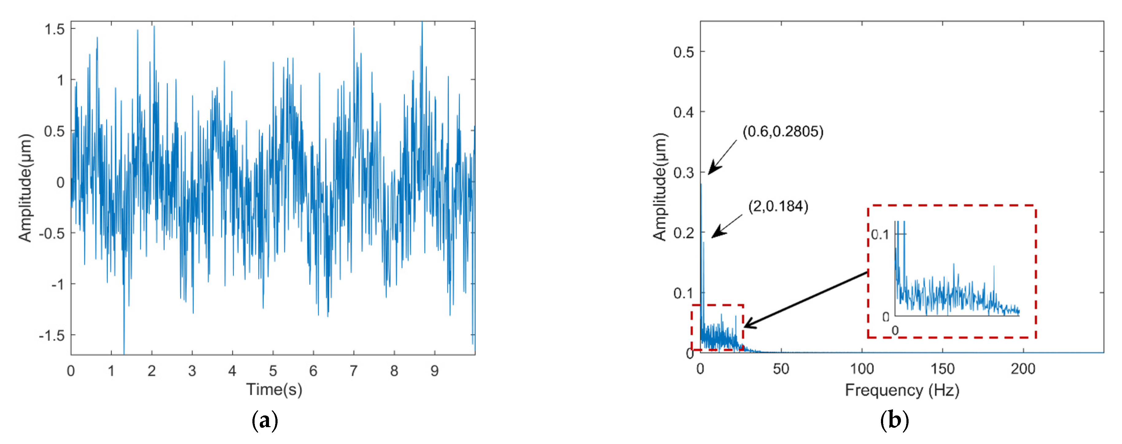
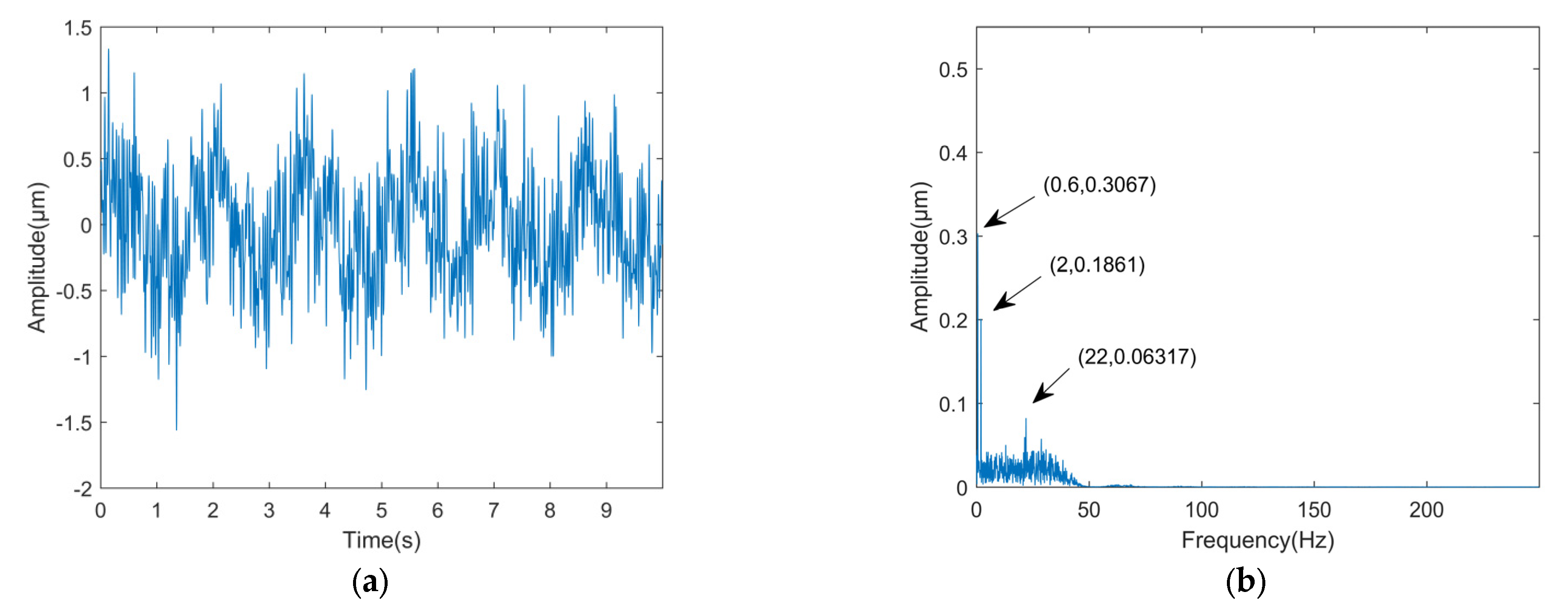
3.2. Vibration Signal Analysis

The simulation graph is shown in Figure 2. Figure 2a,b show the original signal waveform and spectrum, while Figure 2c,d show the waveform and spectrum under strong noise interference. Under strong noise interference, the periodic pulses reflecting the fault characteristics are obliterated. In Figure 2d, it is also not possible to identify the obvious shock components, making it difficult to determine the type of fault.

3.3. Noise Reduction Based on SSA–VMD–SVD

3.3.1. Fitness Function

Entropy, as a measure of signal disorder, can be used as a fitness function for SSA–VMD. EE, SE, and PE can all be used as a fitness function. The lowest entropy value is used as the basis for preferring the parameters. Therefore, in order to reduce the computational cost of the algorithm, only the running times of the different types of entropies are compared. The results are shown in Table 1. It can be seen that the running time and iteration times of EE are the smallest among the three kinds of entropies, while their corresponding optimal parameters are similar, so the EE is used as the final fitness function.

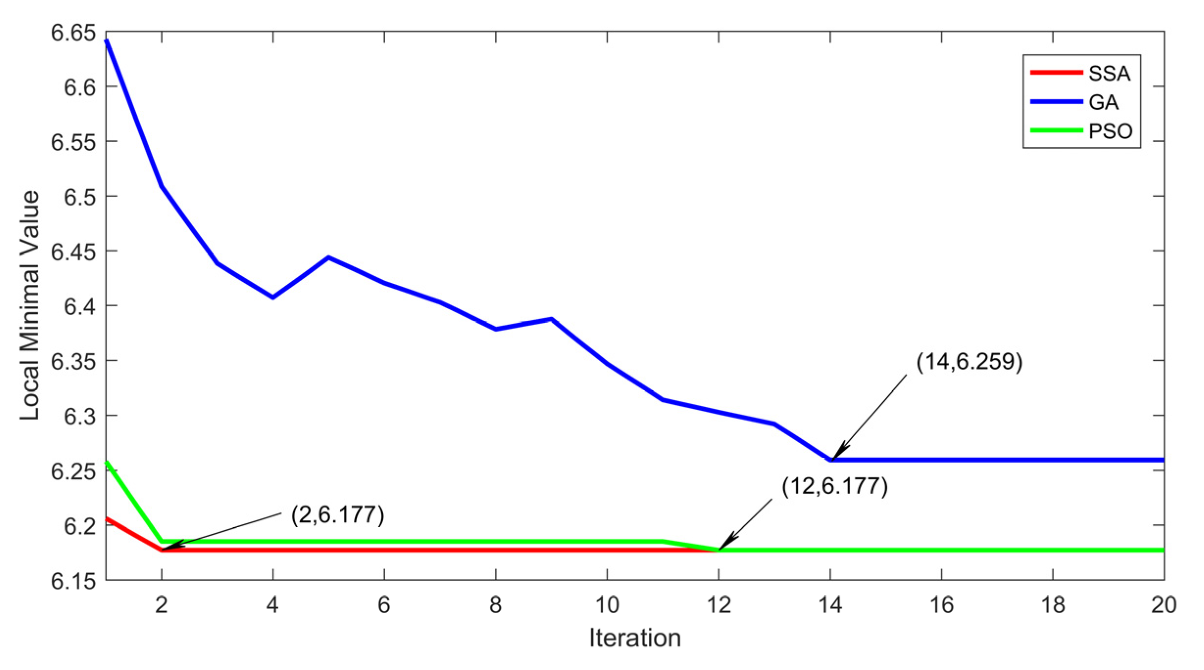
3.3.2. Optimization Algorithms
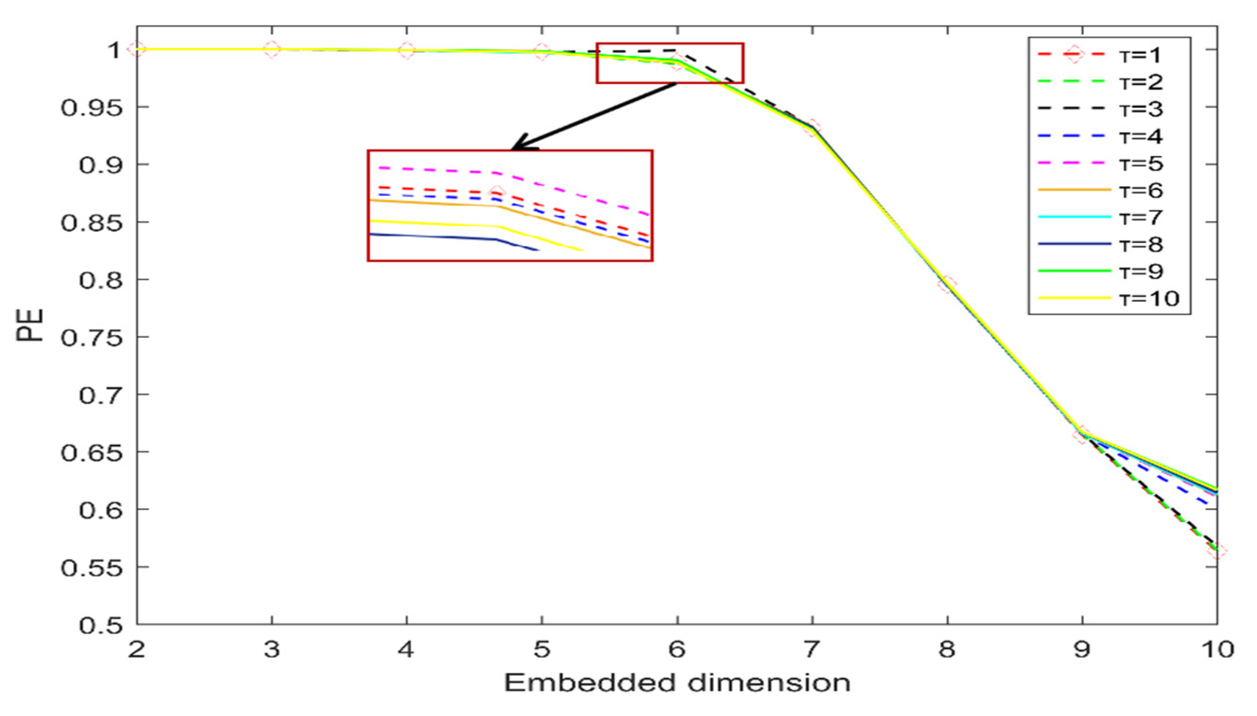
To highlight the global search capability of SSA algorithm, SSA is compared with GA and PSO. Using the EE as the fitness function and setting the same population size, number of iterations, and range of optimization parameters, the optimization results are shown in Figure 3.
As can be seen from Figure 3, in the process of SSA optimization, the local minimum 6.177 appears in the second iteration, and the output parameter is [2853, 10]. In the process of PSO optimization, the local minimum 6.177 appears in the 12th iteration, and the output parameter is [2854, 10]. The local minimum value 6.259 in GA optimization appears in the 14th iteration, and the output parameter is [2902, 10]. When the output parameter value is close to the decomposition effect, the number of iterations of SSA is small and the fitness function is small, which proves that the convergence speed and global search ability of SSA are superior to GA and PSO.
Considering the randomness of the algorithm, the SSA-VMD algorithm with the envelope entropy as the fitness function was optimized for 10 times and the average value was taken as the output result, and the parameter combination was [2853, 10].

3.3.3. PE Parameter

The embedding dimension of the PE affects the construction accuracy, the embedding dimension m usually ranges from 3 to 7, and the delay time τ is usually set to 1 [40]. In order to select the PE parameters suitable for the pressure pulsation signal of the pumped storage unit, the PE values of the simulated signal with m [2, 10] and τ [1, 10] are compared and analyzed. The results are shown in Figure 4.
As can be seen from the Figure 4, when the embedding dimension is a fixed value, the curves in the figure mostly overlap.
Proof. 
The delay time has little effect on the PE value, and sufficient information can be obtained with a delay time of 1. □
Therefore, the delay time τ of 1 is chosen in this paper. When the embedding dimension m is [2,6], the entropy value remains within a stable and small difference. When the m is greater than or equal to 7, the PE value appears to be more volatile, which will cause some interference to the evaluation of the random degree of the signal. Considering the length of the data, the m should be as large as possible without distortion, so the m is chosen to be 6 and the τ is 1.

3.3.4. The Comparison of Entropy

Entropy can distinguish between the noise component and the effective component to achieve primary noise reduction of the simulated signal [41]. The PE, SE, and EE are combined with VMD for a single noise reduction comparison respectively. The correlation coefficient and mean square error were also introduced to reflect the relationship between the noise-reduced signal and the original signal to evaluate the noise reduction effect of the PE. The calculation results are shown in Table 2.
As seen in Table 2, the correlation coefficient of the VMD–PE processed signal is the largest and the mean square error is the smallest, and the noise reduction preserves the original signal more completely. It proves that PE has the best noise reduction effect among the three entropies.

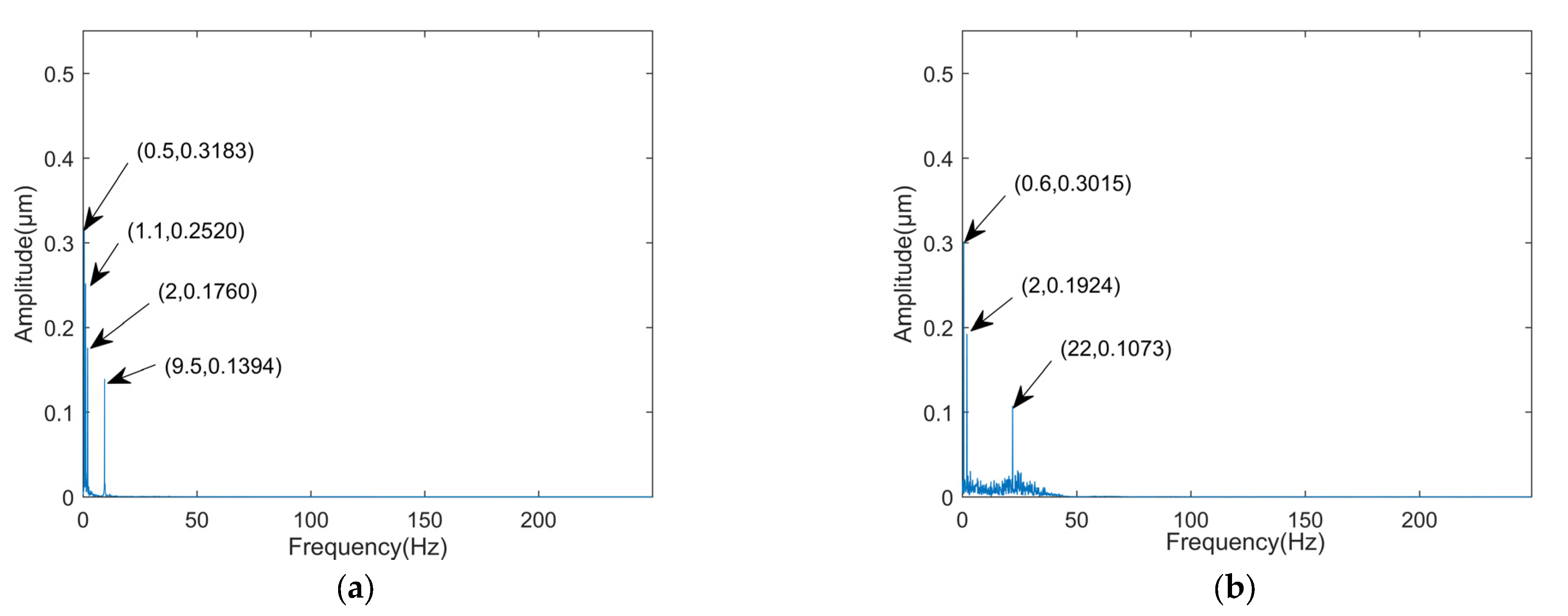
3.3.5. Simulation Results

With the above parameter discussion, the SSA–VMD–SVD processed waveform and spectrum are obtained. As seen in Figure 5a, the processed signal waveform becomes smooth and regular, with a large amount of noise removed without distortion. From Figure 5b, it can be seen that the amplitude of the spectral lines representing the shock component is strong. The f1, f2, and f3 frequencies reflecting the fault characteristics were basically extracted effectively. This demonstrates that the SSA–VMD–SVD decomposition works well and that there is no mode mixing problem.

4. Discussion

4.1. Comparison of Methods

4.1.1. Comparative Analysis

In order to highlight the effectiveness and reliability of the proposed method, other methods are used for noise reduction and feature extraction comparison. The signal processing method considering time domain or frequency domain cannot adapt to the non-stationarity and non-linearity of pressure pulsation signal. The representative time-frequency signal decomposition method (CEEMD ALIF VMD) combined with PE was selected to carry out the primary noise reduction of the simulation signal. However, the effect of primary denoising on complex signal denoising and feature extraction is not ideal, so on the basis of primary denoising, SVD secondary denoising process is added. Figure 6, Figure 7, Figure 8 and Figure 9 show the simulated signal plots after CEEMD–PE, VMD–PE, ALIF–PE, and ALIF–SVD processing respectively.
The white noise added to the CEEMD decomposition is set at 0.2 times the standard deviation and 100 times the number of sets [42]. Due to the reconstruction bias caused by the addition of white noise resulting in some noise remaining in the signal after CEEMD processing, only two feature components are effectively extracted in Figure 6b. As seen in Figure 7 and Figure 8, the burr is reduced in the waveform plots Figure 7a and Figure 8a after VMD–PE and ALIF–PE processing, but the similarity to the original signal Figure 5a is not high. In Figure 7b and 8b, the three feature components are all extracted but the feature components are not accurate enough, there is bottom noise in the 0–50 Hz band, and the noise reduction effect is not satisfactory. The ALIF–SVD processed Figure 9a has a large amount of noise removed but appears distorted. In Figure 9b, only two low-frequency components are effectively extracted, and the full information reflecting the fault characteristics is not completely extracted.

4.1.2. Effectiveness Evaluation

To make the above conclusions more convincing, the correlation coefficient and mean square error were introduced to reflect the relationship between the processed signal and the original signal, and the results were calculated as shown in Table 3.
As can be seen from Table 3, the correlation coefficient after VMD–SVD processing is the highest and the mean square error is the lowest among the methods, which proves that this method has the highest similarity to the original signal after denoising and reconstruction, retains the highest integrity of valid information, and is more effective for the extraction of early weak faults in the draft tube.

4.2. Analysis of Variable Working Conditions
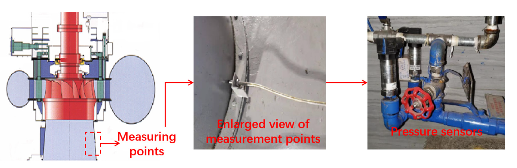
In order to prove that VMD–SVD is not only suitable for noise reduction of vibration signal under single working conditions and fixed noise, change the characteristic frequency under the condition of invariable noise and change the noise size under the condition of invariable characteristic frequency, respectively, to demonstrate the applicability of the method under the condition of variable working conditions and random noise interference.
Construction of simulated signal B with the same noise but different frequencies:
      X 1 =     0.35 · sin ( 2 π t   f 1 ) + 0.3 · sin ( 2 π t   f 2 ) + 0.2 sin · ( 2 π t   f 3 ) + 0.2 sin · ( 2 π t   f 3 ) X 2 = rand   ( 1 ,   5000 ) X t = X 1 + X 2
where f 1 is 0.5 Hz, f 2 is 1.1 Hz, and f 3 is 2 Hz; f 4 is 9.5 Hz.
Construction of simulated signal C with the same frequency but different noise:
    X 1 =     0.3 · sin ( 2 π t   f 1 ) + 0.2 · sin ( 2 π t   f 2 ) + 0.1 sin · ( 2 π t   f 3 ) X 2 = 0.5   rand   ( 1 ,   5000 )   X t = X 1 + X 2
where f 1 is 0.6 Hz, f 2 is 2 Hz, and f 3 is 22 Hz.
The constructed signals were subjected to VMD–SVD processing and the corresponding spectrums were obtained as shown in Figure 10. The correlation coefficients and mean square errors of the three signals after VMD–SVD processing were compared and the results are shown in Table 4.
As can be seen from Figure 10 and Table 4, the characteristic frequencies of signals B and C are basically extracted effectively, and the reconstructed signals maintain a good correlation with the original signals. This demonstrates that VMD–SVD is not only applicable to the noise reduction of vibration signals under single working conditions and fixed noise.

4.3. Examples

In order to verify the effectiveness of the algorithm in this paper, a pumped storage power plant draft tube pressure pulsation signal is used as an example for the unit test. The signal is collected using an AK–4D pressure sensor number N2186, as shown in Figure 11. The unit model is HLNTP–LJ–512, the rated output is 306.1 MW, the rated speed is 300 r/min, the sampling frequency is 500 Hz, and the number of intercepted data points is 5000. Figure 12 shows the measured pressure pulsation signal of a pumped storage power station, and the signal waveform plot is homogenized.
As can be seen in Figure 12a, there is obviously non-periodic noise interference in the signal waveform, and the periodic pulse reflecting the characteristics of the fault is completely masked. As can be seen in Figure 12b, there are some spectral peaks in the middle and high frequency bands but there is no regularity, and there are many interference spectral lines around, making it difficult to accurately determine the cause of the unit fault.
The actual data were processed according to the simulation experiment of VMD–SVD. Figure 13a,b show the waveforms and spectrums after VMD–SVD processing, respectively. From Figure 13a, it can be seen that the processed signal waveform is smoother, the shock regularity is enhanced, and the interference noise is suppressed to a certain extent. As can be seen in Figure 13b, low frequency amplitudes that could not be identified before denoising appear, and the surrounding interference spectral lines are effectively removed. The shock component of X = 0.61 is consistent with the low frequency of the draft tube vortex band, and the shock component of X = 4.5 is close to the rotation frequency of the unit (as shown in the red dashed box), which meets the characteristics of the pressure pulsation of the draft tube vortex band. This proves that the fault characteristics masked by noise are effectively stripped out. The above analysis fully proves that the method in this paper can achieve effective extraction of early faint faults in pressure pulsation of pumped storage units.

5. Conclusions

Against the background of strong noise interference and variable operating conditions of pumped storage units, and in view of the difficulty in extracting the early weak fault characteristics of pressure pulsations of pumped storage units, this paper proposes a sparrow-based optimization VMD combined with SVD for pressure pulsation noise reduction of pumped storage units, with the following conclusions.
(1)
Applying the SSA algorithm with envelope entropy as the fitness function to the parameter decomposition of VMD overcomes the shortcomings of manual parameter selection of VMD and realizes the adaptive decomposition of VMD.
(2)
The choice of the combined VMD–SVD noise reduction method effectively avoids the problem of post-reconstruction noise interference and can achieve good results in non-stationary signal decomposition.
(3)
Through simulation comparison with CEEMD–PE, VMD–PE, ALIF–PE, and ALIF–SVD, it is proved that the noise reduction method of VMD–SVD can effectively remove noise, achieve the extraction of low frequency fault characteristics of pressure pulsation of pumped storage units under strong noise disturbance, and enhance fault-related characteristics.

Author Contributions

Supervision, writing—original draft preparation, Conceptualization, Y.R.; methodology, writing—original draft preparation, L.Z.; visualization, J.C.; formal analysis, J.L.; writing—review and editing, P.L.; data curation, R.Q., X.Y. and S.H.; software, X.L.; validation, investigation, C.C.; resources, H.C. All authors have read and agreed to the published version of the manuscript.

Funding

This research was funded by “Henan Province Key R & D and Promotion Project (Science and Technology Research), grant number No. 212102311054” and the Training Program for Young Key Teachers in Colleges and Universities of Henan Province, grant number No. 2019GGJS097, as well as the Hunan Key Laboratory of Renewable Energy Power Technology (Changsha University of Technology) Open Fund Project, grant number No. 2016ZNDL001.

Institutional Review Board Statement

Not applicable.

Informed Consent Statement

Not applicable.

Data Availability Statement

The data that support the findings of this study are available from the corresponding author upon reasonable request.

Conflicts of Interest

The authors declare no conflict of interest.

References

  1. Han, T.; Li, Y.F.; Qian, M. A Hybrid Generalization Network for Intelligent Fault Diagnosis of Rotating Machinery Under Unseen Working Conditions. IEEE Trans. Instrum. Meas. 2021, 70, 1–11. [Google Scholar] [CrossRef]
  2. Cai, B.; Hao, K.; Wang, Z.; Yang, C.; Kong, X.; Liu, Z.; Ji, R.; Liu, Y. Data-driven early fault diagnostic methodology of permanent magnet synchronous motor. Expert Syst. Appl. 2021, 177, 115000. [Google Scholar] [CrossRef]
  3. Liu, T.; Wang, C.; Chen, Z.; Chen, F.; Bi, H.; Luo, Y.; Wang, Z. Analysis of flow characteristics in pumped storage unit during start-up in turbine mode. J. Phys. Conf. Ser. 2021, 1985, 012051. [Google Scholar] [CrossRef]
  4. Jowsey, E. A new basis for assessing the sustainability of natural resources. Energy 2007, 32, 906–911. [Google Scholar] [CrossRef]
  5. Feng, Z.; Chu, F. Nonstationary Vibration Signal Analysis of a Hydroturbine Based on Adaptive Chirplet Decomposition. Struct. Health Monit. Int. J. 2007, 6, 265–279. [Google Scholar] [CrossRef]
  6. Cai, B.; Liu, Y.; Xie, M. A Dynamic-Bayesian-Network-Based Fault Diagnosis Methodology Considering Transient and Intermittent Faults. IEEE Trans. Autom. Sci. Eng. 2017, 6, 11289–11300. [Google Scholar] [CrossRef]
  7. Ren, Y.; Huang, J.; Hu, L.-M.; Chen, H.-P.; Li, X.-K. Research on Fault Feature Extraction of Hydropower Units Based on Adaptive Stochastic Resonance and Fourier Decomposition Method. Shock Vib. 2021, 2021, 6640040. [Google Scholar] [CrossRef]
  8. Delina, M.; Nurhusni, P.A. Feature extraction of noise signal in motorcycle by Fast Fourier Transform. J. Phys. Conf. Ser. 2021, 1869, 12198. [Google Scholar] [CrossRef]
  9. Guan, S.; Wang, X.; Hua, L.; Li, L. Quantitative ultrasonic testing for near-surface defects of large ring forgings using feature extraction and GA-SVM. Appl. Acoust. 2021, 173, 107714. [Google Scholar] [CrossRef]
  10. Rybak, G.; Strzecha, K. Short-Time Fourier Transform Based on Metaprogramming and the Stockham Optimization Method. Sensors 2021, 21, 4123. [Google Scholar] [CrossRef]
  11. Chui, C.K.; Jiang, Q.; Li, L.; Lu, J. Analysis of an adaptive short-time Fourier transform-based multicomponent signal separation method derived from linear chirp local approximation. J. Comput. Appl. Math. 2021, 396, 113607. [Google Scholar] [CrossRef]
  12. Li, Y.; Wang, Z.; Li, Z.; Li, H. Research on Gear Signal Fault Diagnosis Based on Wavelet Transform Denoising. J. Phys. Conf. Ser. 2021, 1971, 012074. [Google Scholar] [CrossRef]
  13. Zhang, K.; Ma, C.; Xu, Y.; Chen, P.; Du, J. Feature extraction method based on adaptive and concise empirical wavelet transform and its applications in bearing fault diagnosis. Measurement 2021, 172, 108976. [Google Scholar] [CrossRef]
  14. Zhang, K.; Tian, W.; Chen, P.; Ma, C.; Xu, Y. Sparsity-guided multi-scale empirical wavelet transform and its application in fault diagnosis of rolling bearings. J. Braz. Soc. Mech. Sci. Eng. 2021, 43, 1–17. [Google Scholar] [CrossRef]
  15. Pal, S.; Mitra, M. Empirical mode decomposition based ECG enhancement and QRS detection. Comput. Biol. Med. 2012, 42, 83–92. [Google Scholar] [CrossRef]
  16. Jiang, Z.; Wu, Y.; Li, J.; Liu, Y.; Xu, X. Application of EMD and 1.5-dimensional spectrum in fault feature extraction of rolling bearing. J. Eng. 2019, 2019, 8843–8847. [Google Scholar] [CrossRef]
  17. Chen, Y.; Sun, J. Fault Diagnosis of Rolling Bearing Based on EEMD and PSO-SVM. Electr. Power Sci. Eng. 2016, 32, 47. [Google Scholar]
  18. Liu, X.; Zhang, X.; Luan, Z.; Xu, X. Rolling bearing fault diagnosis based on EEMD sample entropy and PNN. J. Eng. 2019, 2019, 8696–8700. [Google Scholar] [CrossRef]
  19. Wang, W.; Chen, Q.; Yan, D.; Geng, D. A novel comprehensive evaluation method of the draft tube pressure pulsation of Francis turbine based on EEMD and information entropy. Mech. Syst. Signal Process. 2019, 116, 772–786. [Google Scholar] [CrossRef]
  20. An, X.; Zeng, H.; Li, C. Demodulation analysis based on adaptive local iterative filtering for bearing fault diagnosis. Measurement. 2016, 94, 554–560. [Google Scholar] [CrossRef]
  21. Zhao, L.; Liu, X.; Lou, L. The feature extraction method of non-stationary vibration signal based on SVD-complex analytical wavelet demodulation. Zhendong Ceshi Yu Zhenduan/J. Vib. Meas. Diagn. 2015, 35, 672–676. [Google Scholar]
  22. Ren, Y.; Liu, P.; Hu, L.; Huang, J.; Huang, S. Research on Noise Reduction Method of Pressure Pulsation Signal of Draft Tube of Hydropower Unit Based on ALIF-SVD. Shock Vib. 2021, 2021, 5580319. [Google Scholar] [CrossRef]
  23. Bai, Y.; Liu, M.D.; Ding, L.; Ma, Y.J. Double-layer staged training echo-state networks for wind speed prediction using variational mode decomposition. Appl. Energy 2021, 301, 117461. [Google Scholar] [CrossRef]
  24. Gfa, B.; Hwa, B.; Tqa, B.; Xpa, B.; Hong, W.C. A Transient Electromagnetic Signal Denoising Method Based on An Improved Variational Mode Decomposition Algorithm—ScienceDirect. Measurement 2021, 184, 109815. [Google Scholar]
  25. Zhu, X.; Huang, Z.; Chen, J.; Lu, J. Rolling bearing fault diagnosis method based on VMD and LSSVM. J. Phys. Conf. Ser. 2021, 1792, 12035. [Google Scholar] [CrossRef]
  26. Zhang, Y.; Lian, Z.; Fu, W.; Chen, X. An ESR Quasi-Online Identification Method for the Fractional-Order Capacitor of Forward Converters Based on Variational Mode Decomposition. J. IEEE Trans. Power Electron. 2022, 37, 3685–3690. [Google Scholar] [CrossRef]
  27. Song, X.; Wang, H.; Chen, P. Weighted kurtosis-based VMD and improved frequency-weighted energy operator low-speed bearing-fault diagnosis. Meas. Sci. Technol. 2021, 32, 035016. [Google Scholar] [CrossRef]
  28. Gu, X.; Chen, C. Rolling Bearing Fault Signal Extraction Based on Stochastic Resonance-Based Denoising and VMD. Int. J. Rotating Mach. 2017, 2017, 3595871. [Google Scholar] [CrossRef] [Green Version]
  29. Li, Y.; Cheng, G.; Liu, C.; Chen, X. Study on planetary gear fault diagnosis based on variational mode decomposition and deep neural networks. Measurement 2018, 130, 94–104. [Google Scholar] [CrossRef]
  30. Wen, Y.; Luk, K.; Gazeau, M.; Zhang, G.; Chan, H.; Ba, J. An Empirical Study of Large-Batch Stochastic Gradient Descent with Structured Covariance Noise. arXiv 2019, arXiv:1902.08234. [Google Scholar]
  31. Li, K.; Su, L.; Wu, J.; Wang, H.; Peng, C. A Rolling Bearing Fault Diagnosis Method Based on Variational Mode Decomposition and an Improved Kernel Extreme Learning Machine. Appl. Sci. 2017, 7, 1004. [Google Scholar] [CrossRef] [Green Version]
  32. Lee, Z.J.; Su, S.F.; Chuang, C.C.; Liu, K.H. Genetic algorithm with ant colony optimization (GA-ACO) for multiple sequence alignment. Appl. Soft Comput. 2008, 8, 55–78. [Google Scholar] [CrossRef]
  33. Zhou, S.; Xie, H.; Zhang, C.; Hua, Y.; Sui, X. Wavefront-Shaping Focusing Based on a Modified Sparrow Search Algorithm. Opt.-Int. J. Light Electron Opt. 2021, 244, 167516. [Google Scholar] [CrossRef]
  34. Litvinov, I.; Shtork, S.; Gorelikov, E.; Mitryakov, A.; Hanjalic, K. Unsteady regimes and pressure pulsations in draft tube of a model hydro turbine in a range of off-design conditions. Exp. Therm. Fluid Sci. Int. J. Exp. Heat Transf. Thermodyn. Fluid Mech. 2018, 91, 410–422. [Google Scholar] [CrossRef]
  35. Su, W.T.; Binama, M.; Li, Y.; Zhao, Y. Study on the method of reducing the pressure fluctuation of hydraulic turbine by optimizing the draft tube pressure distribution. Renew. Energy 2020, 162, 550–560. [Google Scholar] [CrossRef]
  36. Dragomiretskiy, K.; Zosso, D. Variational Mode Decomposition. IEEE Trans. Signal Process. 2014, 62, 531–544. [Google Scholar] [CrossRef]
  37. Hua, L.; Tao, L.; Xing, W.; Qing, C. Application of EEMD and improved frequency band entropy in bearing fault feature extraction. ISA Trans. 2018, 88, 170–185. [Google Scholar]
  38. Cao, Y.; Tung, W.; Gao, J.B.; Protopopescu, V.A.; Hively, L.M. Detecting dynamical changes in time series using the permutation entropy. Phys. Rev. E 2004, 70, 46217. [Google Scholar] [CrossRef] [Green Version]
  39. Jiang, H.; Chen, J.; Dong, G.; Liu, T.; Chen, G. Study on Hankel matrix-based SVD and its application in rolling element bearing fault diagnosis. Mech. Syst. Signal Process. 2015, 52–53, 338–359. [Google Scholar] [CrossRef]
  40. Zanin, M.; Zunino, L.; Rosso, O.A.; Papo, D. Permutation Entropy and Its Main Biomedical and Econophysics Applications: A Review. Entropy 2012, 14, 1553–1577. [Google Scholar] [CrossRef]
  41. Li, Y.; Gao, X.; Wang, L. Reverse Dispersion Entropy: A New Complexity Measure for Sensor Signal. Sensors 2019, 19, 5203. [Google Scholar] [CrossRef] [PubMed] [Green Version]
  42. Yeh, J.R.; Shieh, J.S.; Huang, N.E. Complementary ensemble empirical mode decomposition: A novel noise enhanced data analysis method. Adv. Adapt. Data Anal. 2011, 2, 135–156. [Google Scholar] [CrossRef]
Figure 1. The framework flow chart of the proposed method.
Energies 15 02073 g001
Figure 2. Simulated signal waveform and spectrum (a) Original signal waveform diagram; (b) Spectrum of the original signal; (c) Noise added signal waveform diagram; (d) Noise added signal spectrum.
Energies 15 02073 g002
Figure 3. Iterative adaptation under different algorithms.
Energies 15 02073 g003
Figure 4. The relationship between the PE parameters.
Energies 15 02073 g004
Figure 5. Simulated signal after SSA-VMD–SVD processing. (a) Waveform diagram after noise reduction; (b) Spectrum after noise reduction.
Energies 15 02073 g005
Figure 6. Simulated signal after CEEMD–PE processing. (a) Waveform diagram after noise reduction; (b) Spectrum after noise reduction.
Energies 15 02073 g006
Figure 7. Simulated signal after VMD–PE processing. (a) Waveform diagram after noise reduction; (b) Spectrum after noise reduction.
Energies 15 02073 g007
Figure 8. Simulated signal after ALIF–PE processing. (a) Waveform diagram after noise reduction; (b) Spectrum after noise reduction.
Energies 15 02073 g008
Figure 9. Simulated signal after ALIF–SVD processing. (a) Waveform diagram after noise reduction; (b) Spectrum after noise reduction.
Energies 15 02073 g009
Figure 10. Spectra of the two simulated signals after VMD–SVD processing. (a) Spectrum of signal B after noise reduction; (b) Spectrum of signal C after noise reduction.
Energies 15 02073 g010
Figure 11. Sensor arrangement measurement diagram.
Energies 15 02073 g011
Figure 12. Measured pressure pulsation signal at a pumped storage power station. (a) Signal waveform diagram; (b) Signal spectrum.
Energies 15 02073 g012
Figure 13. Graph of the actual data signal after VMD–SVD processing. (a) Waveform diagram after noise reduction; (b) Spectrum after noise reduction.
Energies 15 02073 g013
Table 1. Table of optimization parameters for different fitness functions.
Fitness Functions[a, K]Number of IterationsMinimum Entropy ValueRunning Time (s)
EE[2853, 10]26.17664705
PE[2996, 10]20.456217150
SE[2898, 10]50.222110762
Table 2. Noise reduction test with three types of entropy.
Feature Extraction MethodsCorrelation CoefficientMean Square Error
VMD-PE0.62100.3169
VMD-SE0.49310.4368
VMD-EE0.49450.4494
Table 3. Assessment table for different methods of noise reduction.
Correlation CoefficientMean Square Error
Noisy signals0.24281.0068
CEEMD–PE0.51230.4227
VMD–PE0.62100.3169
ALIF–PE0.70240.2595
ALIF–SVD0.93600.0940
VMD–SVD0.96140.0732
Table 4. Table of evaluation indicators for different signals.
SignalCorrelation CoefficientMean Square Error
A0.96140.0732
B0.97760.0901
C0.99420.0285
Publisher’s Note: MDPI stays neutral with regard to jurisdictional claims in published maps and institutional affiliations.

