Voltage Fluctuations and Flicker in Prosumer PV Installation

Abstract

In this paper, we present problems connected with voltage fluctuations in low-voltage networks caused by small PV sources installed in an LV network. For the purpose of analysis, high-resolution data gathered at the output of real PV sources for 4 months in 2 locations are used. Data are processed to analyze the impact of different network parameters on voltage fluctuations and voltage flicker. The resulting values of flicker and fluctuations are given so the assessment of the impact of PV sources can be made before the connection of new sources to the power grid. Moreover, the methodology of analysis is presented in detail so the impact of similar PV sources on voltage could be analyzed. Finally, general conclusions connected with measurement, analysis, and mitigation are given.

1. Introduction

The development of the power system network observed in the last decade is motivated by the need of the CO2 emission reduction. In particular, the reduction of fuel consumed in power plants and vehicles. As a result, many active elements such as small renewable energy sources, electric vehicle charging stations, energy sources, and others are installed in distribution system network. As a consequence, the direction of power flow is changed and new challenges connected with ensuring proper power quality arise—increased harmonic distortion, higher voltage fluctuations, and voltage flicker. Additionally, problems with unwanted islanding of power sources and other problems are present [1,2].

Recently, attention has been paid to an increased voltage level in power networks with a high share of renewable energy sources and the need to develop new methods of voltage regulations and methods of sources control [3,4]. The literature contains a great amount of information connected with the impact of PV sources on power flow or different issues, e.g., balancing the power network with renewable energy sources or the impact of PV sources on the operation of tap changer of transformer [5,6]. Unfortunately, the literature contains a limited number of publications connected with voltage variability caused by renewables, and the existing information considers relatively big time intervals, e.g., 1 min or second, which is not enough to analyze flicker factors, particularly in low-voltage systems [7]. The literature contains interesting information connected with the modeling of clouds and their impact on PV plants, but the presented models are developed for relatively big energy sources above 1 MVA [8]. Because of the complex interaction between many different inverters, one cannot make use of the information in the context of small-scale, prosumer PV sources. Few studies related to voltage fluctuations in small PV installations draw attention to the existence of the problem and indicate the correlation between power plant power and fluctuations; however, no details are given. It is claimed in [9,10,11,12] that in general, the risk of voltage flicker is more likely in places with a high share of renewables. Norm [9] does not provide information regarding flicker caused by PV sources and claims that in case of situations not presented in the norm one needs to perform simulations. Unfortunately, the task is difficult since one needs to have professional equipment for data gathering and professional software for data analysis. Moreover, one needs to have basic knowledge of electrical power engineering, data processing, and analytical skills. As a result of many challenges, there are no practical and reliable rules for predicting voltage flicker and fluctuations caused by prosumers PV sources.

Finally, one needs to realize that literature presents information from all over the world and, therefore, big differences may occur due to different cloud characteristics, which are the main source of PV power fluctuations.

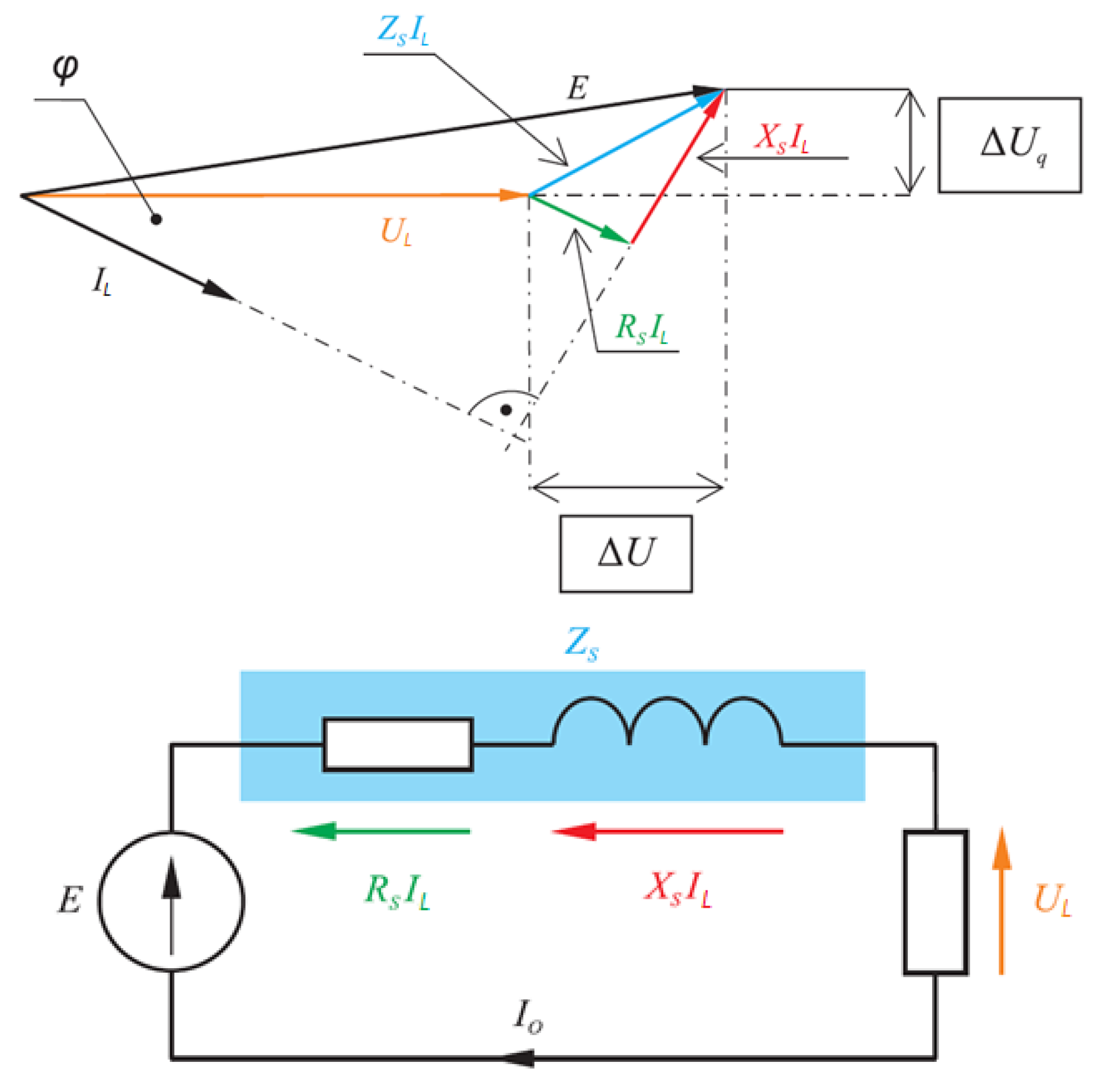
2. Voltage Fluctuations in a Power System Network

The voltage level is changed every time; the current flows through an impedance. At the low-voltage level, typically only series elements of the lumped-element model—resistance and reactance—are considered. Voltage loss caused by resistance is in phase with the current I_L and is equal to R_SI_L (Figure 1). The voltage loss caused by reactance is perpendicular to the current I_L and is equal to X_SI_L (Figure 1). The relative voltage drop caused by the impedance can be described as [13]:

$$\frac{E-U_L}{U_L}\approx \frac{\Delta U_L}{U_L}=R_S\frac{P}{U_L^2}+X_S\frac{Q}{U_L^2}$$

(1)

Voltage fluctuations are the result of dynamic changes of load or generation. An example of the dynamic load is an electric wood saw, which alternately work at idle load and heavy load conditions (engine stall) or welding machines. An example of a generator characterized by high variability are photovoltaic and wind sources [14].

Voltage fluctuations can be described in different ways. If the frequency of voltage fluctuations is lower than 1 Hz, the factor used to describe voltage changes is the amplitude of voltage deviation—a given by formula (2).

$$a=\frac{\sqrt{3}\Delta I·R·cos\phi +\sqrt{3} \Delta I·X·sin\phi +}{U}=\frac{\Delta P}{U^2}R+\frac{\Delta Q}{U^2}X$$

$$=\frac{\Delta Scos\phi }{U}·\frac{1.1U^2}{S_{kQ}^{″}}cos\psi +\frac{\Delta Ssin\phi }{U}·\frac{1.1U^2}{S_{kQ}^{″}}sin\psi =$$

(2)

$$=1.1\frac{\Delta S}{S_{kQ}^{″}}cos\phi ·cos\psi +1.1\frac{\Delta S}{S_{kQ}^{″}}sin\phi ·sin\psi =1.1\frac{\Delta S}{S_{kQ}^{″}}\cos \left(\psi -\phi \right)$$

where:

• φ—the angle between real and apparent power,
• ψ—the angle that describes the impedance of supply line,
• $\Delta I/\Delta S$—change of consumed or generated current/power, and
• $S_{kQ}^{″}$—short circuit power.

If the frequency of voltage fluctuations is higher than 1 Hz, the factor used to quantify the impact of voltage deviation is the acceptable dose of flicker [15]. To calculate the dose of flicker, one can use different factors—Pst and Plt used in Europe and analyzed in the paper or V10 in Arabic countries. The Pst factor can be compared with the filter imitating the perception of light flicker caused by the voltage changes by the statistical human eye. The description of the filter can be found in many different publications, e.g., [16]. One needs to underline that in real cases, the differentiation of factors, which can be used to describe the voltage fluctuations, is difficult since many different sources of flicker accumulate over time. To identify the sources of voltage flicker, one can perform an analysis of the correlation between flicker and variable elements of the power system [17]. Voltage fluctuations have a negative impact on loads connected to a power system. Among the negative impact of voltage flicker, one can mention the negative impact on [13,18,19]:

-

electrical machines—voltage fluctuations causing changes of electrical torque, which can lead to engine vibrations, which in turn can lead to failure and can shorten the engine life. Moreover, the torque variation leads to increased losses and deterioration of product quality,

-

power electronic—voltage fluctuation can cause the reduction of power factor and generation of noncharacteristic harmonics and interharmonics,

-

devices for electrolysis—shortening the life of electrodes,

-

electrothermal devices—replacement of the effectiveness,

-

light—a variation of the light flux,

-

uninterruptible power sources (UPS)—unnecessary utilization of the UPS batteries, which increases the power losses.

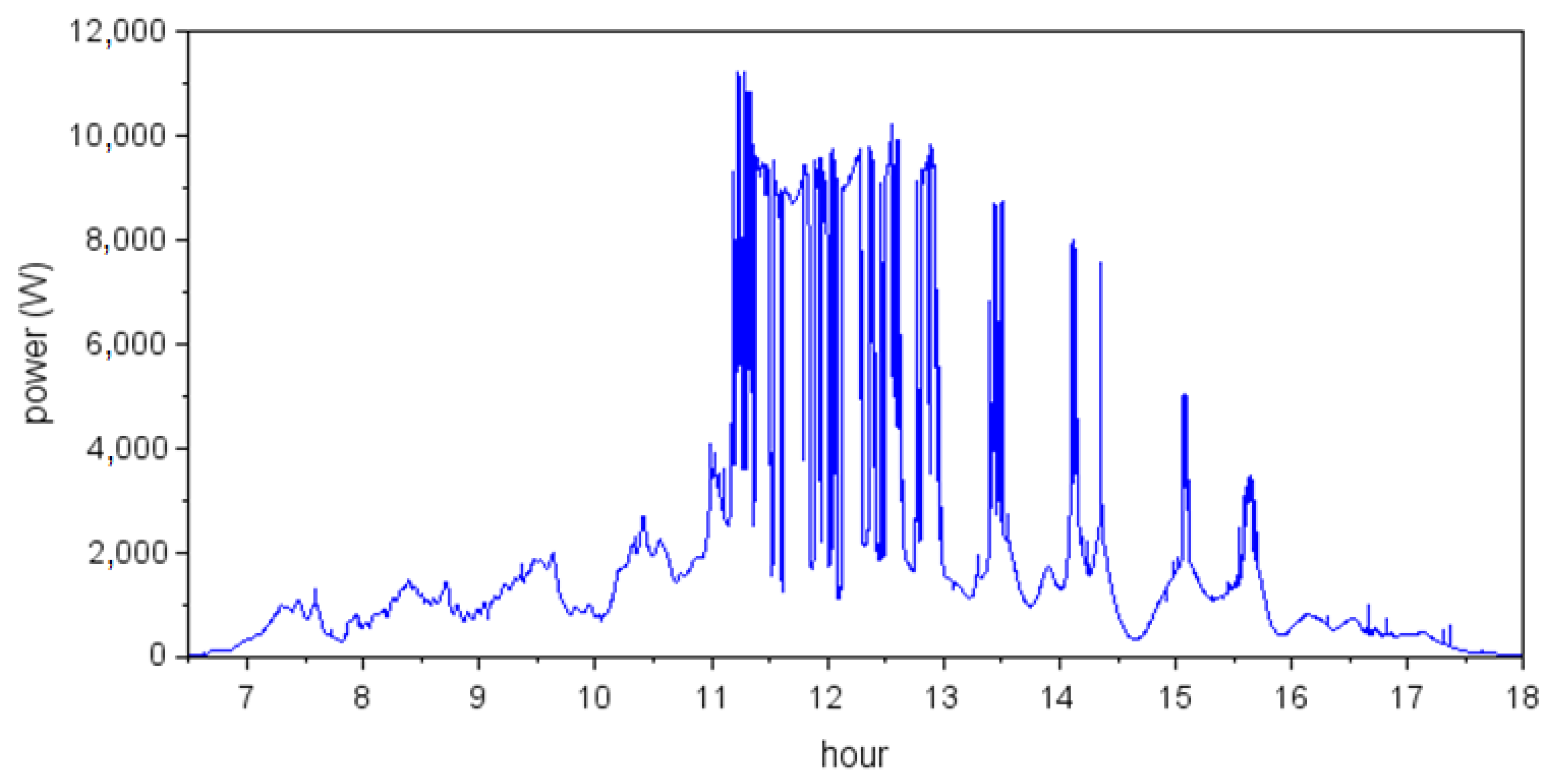
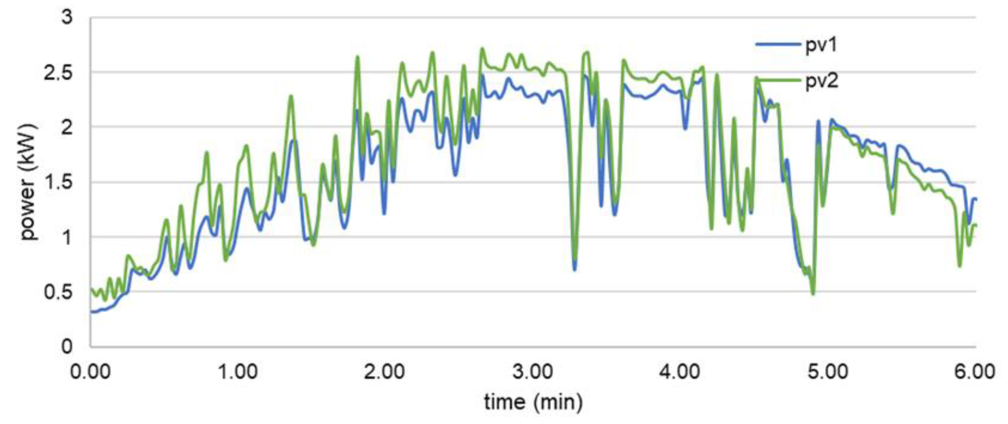
According to the power quality norm IEC 61000-3-3, the Pst factor in the consumer installations should be <1.0, and the Plt factor should be below 0.65. There are different Pst variations—Pst_1min, Pst_5min, and Pst_10min, depending on the observation time window. European norm EN50160 requires that Plt is below 1 for 95% of measurements taken for 1 week. The flicker factor—Pst and Plt in low voltage network are caused by the voltage fluctuations in the MV network, which supply the MV/LV transformer and operation of loads and sources connected to the low voltage side of the transformer. As a result, one cannot simply determine the acceptable rise of flicker factors caused by the new devices since the operating conditions differ significantly. According to the measurement taken by the author in a few 110/15 kV substations, the flicker factors are changing in the vast range. In the case of so-called calm loads, the Pst is approximately 0.1, whereas, in the case of dynamic loads, e.g., industrial or railway or sources, the flicker factor can be in the range of 0.3 to 0.6 or even more depending on the share of dynamic elements of a power system. As a result, the number of PV sources, which can be connected to a low voltage network depends on the voltage parameters of the 110/15 substation, which can be tens of km away. Moreover, one need to underline that with the increasing distance from the 110/15 substation, the electrical impedance increases, and, therefore, the voltage flicker in the MV network close to the MV/LV substation increases as well. Finally, one needs to consider the voltage drop along the impedance of the MV/LV transformer, which depends on the loading on the transformer, e.g., 0.94 % voltage drop in 200 kVA transformer, which transfers power 0.3 Sn (60 kVA) or 2.38% voltage drop in smaller transformer 100 kVA, which transfers 0.6 Sn (also 60 kVA) [20]. Finally, the rise of distance from MV/LV stations has a further negative impact on voltage fluctuations. Despite the electrical parameters, one needs to realize that voltage deviations depend on the moment of operation of sources and loads. When loads and sources are working at the same time, the voltage difference between minimum and maximum operating voltages may rise significantly, e.g., just after the sudden decrease of the PV output, a load is turned on and the voltage drop is amplified. The presented example is particularly important in the context of local regulations connected with the price of electricity. According to regulations in Poland, PV prosumers connected to network before April 2022 can utilize 100% of the output energy when installation is active or make use of the 80% surplus energy any time. In case of PV prosumers connected after April 2022, the surplus energy is sold according to prices on the ‘next day’ market [21]. The sold energy is significantly cheaper than the bought energy, so the prosumer is motivated to consume as much energy when PV installations is active as possible. As a result, the risk that voltage deviation will be amplified increases. At the same time, one needs to know that new regulations require the installation of battery banks, which could be used to mitigate the problem. Unfortunately, at the moment, it is not clear how the batteries should be operated. As a result of the presented factors, the Pst in low voltage networks is often high. Measurements taken in the Netherlands indicate that in the case of approximately 10% of consumers, the Pst is above 1 (the limit defined in EN50160) (Figure 2) [22]. The rise of flicker factor is connected with complaints from electricity consumers, e.g., in Moravia, the region of Czech Republic (~3 mln of citizens), 2000 complaints are noted every year [23].

Theoretically, to verify if the connection of new PV sources will cause violation of flicker, one could estimate the rise of flicker factor resulting from the connection of PV source and add it to background values. However, one needs to consider the correction factor, which results from the complex interaction between the impact of photovoltaic source and background voltage, which is further explained in the article. The background flicker values can be measured by smart meters. Smart meters can be categorized as a 4 quadrant meters for MV/LV substations, intermediate meters, e.g., 2 directional meters for prosumers and high scale loads, and simple 1 direction meters for regular loads [25]. The meters installed in MV/LV substation gather Pst data according to EN50160 norm every 10 min and Plt every 2 h, whereas the simple meters record only Plt every 2 h. The Plt factor allows to determine if the values are within the limits specified by norms; however, the correlation analysis cannot be performed. Finally, in the case of consumer and prosumer installations, the load profile can be estimated using, e.g., artificial combination of synthetic load profiles or profiles recorded by smart meters [26]. The estimated profile can be further used in order to estimate the flicker level.

3. Measurements

Measurements of the PV source output are taken in 2 prosumer, rooftop installations. The nominal power of the first installation is 3.5 kWp and the inverter is Growatt TL3-S, which is further referred to as installation A, whereas the power of the second installation is 10 kWp (further referred to as installation B—Sofar 11 KTL-X. measurements in installation A are taken in the summer months—from 1 June to 1 September, whereas measurements taken in installation B are taken between 20.02 and 20.03.

Measurements in both installations are recorded by the same meter [27]. The meter records electrical parameters in 3 phases, however, because of the small current asymmetry—in the range of 2%, only the total output power is analyzed. Among many recorded parameters, the active power generated by the PV source is analyzed because the small-scale PV sources operate with the unity power factor (only active power is produced) [28].

Despite of the measurement of PV installation, the separate voltage measurements are taken in a few locations—urban areas, in which apartment blocks are the main loads, village areas—where single-family housing are the main loads, and suburban—with both single-family housing and apartment blocks.

Figure 3 presents the output power of PV recorded over one day. As can be observed, in favorable conditions, the output power can exceed the nominal power of installed panels. The rise above nominal power can occur in case of steady favorable environment conditions, e.g., sunny weather and optimum temperature or for a short time when shadow created by the cloud trespass the photovoltaic panels because light passing on panels is intensified—light is passing directly from the sun and additionally from the cloud because part of the light emitted by sun is reflected [29]. The presented phenomena have a negative impact on the voltage flicker since the deviations of voltage at the point of coupling are intensified.

The goal of the following paper is to describe the voltage flicker in normal operating conditions; at the same time, one needs to realize that each inverter may have specific features, which impacts the flicker factor in a specific way. A good example is the inverter startup. The startup of inverter A is presented in Figure 4. Before the inverter starts, one can observe the step rise of the reactive power—at first, from approximately 140 Var to 400 Var, and afterward, the step rise from 400 to 1100 Var, after which one observes the exponential decay of the output reactive power. Moreover, relatively small peaks of active power can be observed <100 W. The step change of power obviously has a negative impact on the flicker factors. The presented rapid changes of power are observed a few times to approximately 10 times over 30 min every day. The startup of inverter B (Figure 5) is also connected with rapid changes of power; however, in this case, the power pulsation is characterized by small power and the disturbance lasts a few hundred seconds.

4. Measurement Analysis

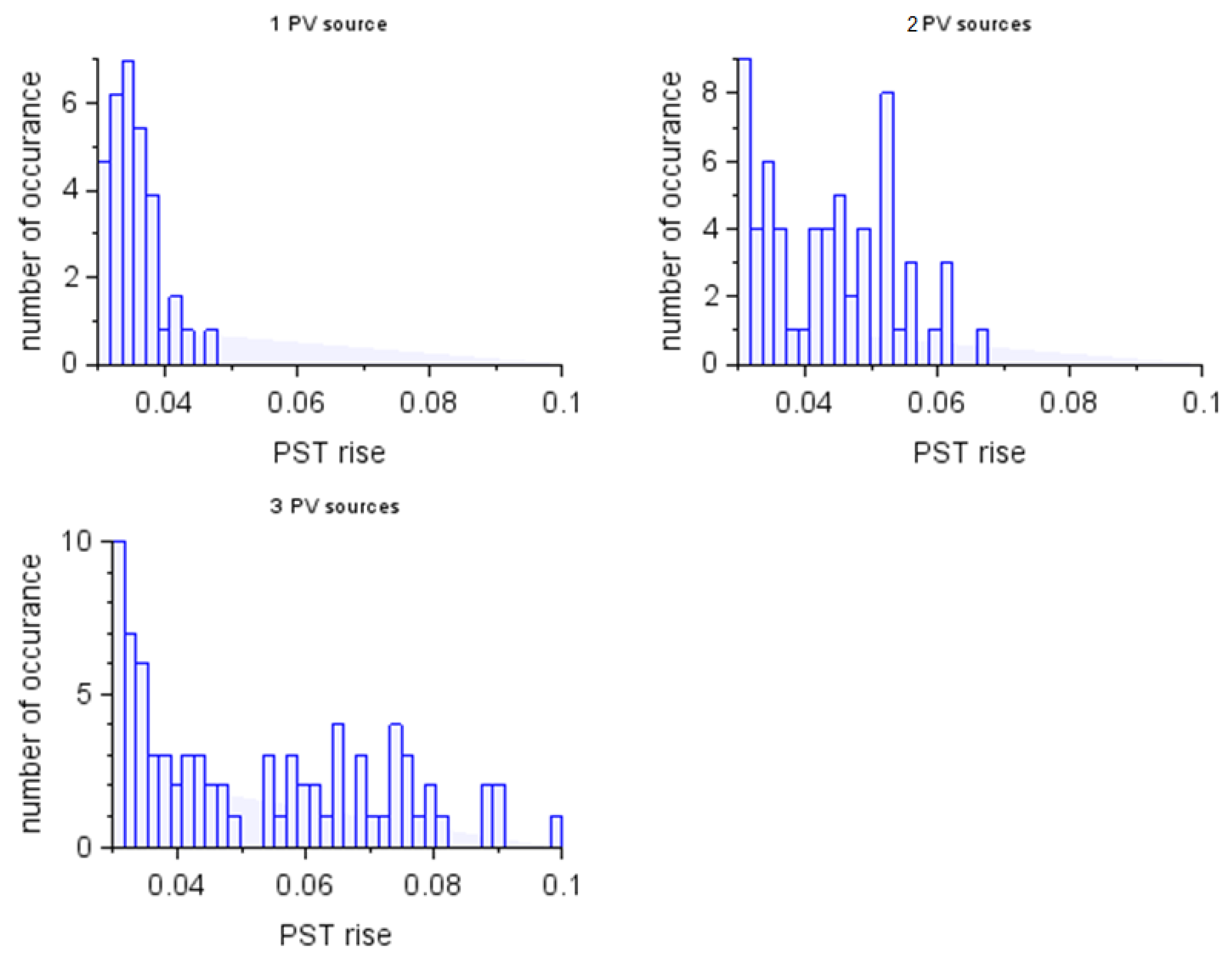
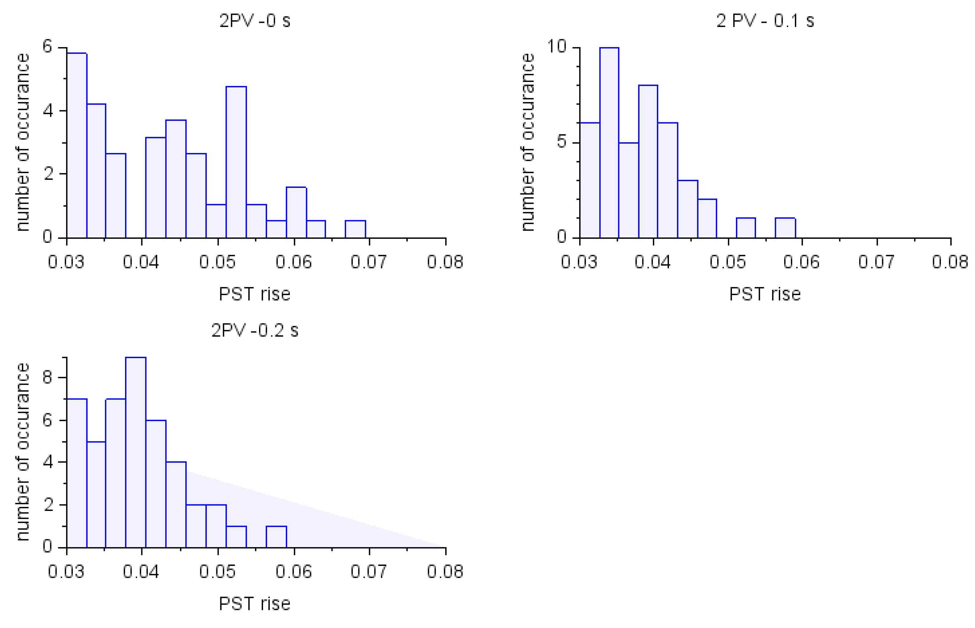
4.1. Impact of PV Sources Connected to Ideal LV Network

Assessment of the impact of PV sources is based on the relation between the PV output power and the rise of voltage in the network. In the initial stage of the research, an impact of different power system parameters is analyzed—impedance, local consumption of power, the output power of PV sources, location of PV source installation, and others. For the case of simplicity, it was assumed that voltage in the network remains constant. Because of the relatively complex mathematical description of the relation between PV output, particularly in the case of a few PV installations in different locations, the relation between output power and voltage is presented as a linear function. The coefficient of the linear function is obtained with the help of simulation software—PowerFactory (Figure 6) and the formula of a linear function. The linear function allows for a simple, intuitive comparison of different parameters.

The a factors of linear functions are presented in

Table 1. Coefficients describing the relationship between voltage and output power.

Length of the Power Lines				Stable Local Consumption (Cable Lengths 250 and 50 m
Lutility [m]	Lconsumer [m]	apv	apcc	Plocal [kW]	apv	apcc
150	50	0.1922	0.0433	0	0.2555	0.17
250	25	0.2133	0.17	5	0.2566	0.1722
250	50	0.2555	0.17	10	0.2577	0.1733
500	50	0.4098	0.3255	15	0.2599	0.1743
750	50	0.562	0.4776	20	0.2621	0.1755
1000	50	0.7007	0.6175	25	0.2644	0.1777

. Analysis of Table 1 allows concluding that the rise of impedance results in the almost linear rise of voltage and that the impedance of the prosumer line can cause a significant rise of the voltage. One needs to underline that norms require proper parameters in the point of connection with the network (referred as PCC); therefore, in some cases, the flicker in prosumer installation may exceed the allowable limits even though the norms requirement are fulfilled. Moreover, one can observe that the level of stable local consumption has a small impact on the voltages in the power line; therefore, the local consumption is not analyzed in the text.

To obtain the voltage in the point of coupling of the PV source with grid, the linear coefficient is multiplied by output power and added to background voltage—230 phase to ground voltage. Obtained RMS voltages are further analyzed in the Flickermeter module is available in PowerFactory software. The flicker meter fulfills the requirement of the IEC 61000-3-7 norm. The method of flicker calculation based on the RMS values is presented in [31].

The a coefficients presented in Table 1 are calculated under nominal voltage level. In case of voltage deviation, the coefficients will change—the higher the voltage is, the smaller is the current needed to transfer the power and, therefore, the smaller the voltage rise is.

Figure 7 presents the impact of line length on the Pst_1min (norm requirements may be connected with longer period Pst, e.g., 10 min) calculated in the power factory software. Presented results are calculated using the output power recorded 17.03 in installation B (Figure 8). As can be seen, the rise of impedance causes the rise of maximum Pst_1min value, which is in the range of 0.1, when the PV source is connected with MV/LV substation by 1 km of 70 mm² cable line. It is worth mentioning that in the case of old rural power lines, even longer lengths and smaller cross-sections can be observed. The rise of the maximum Pst caused by the impedance can be approximated by the linear function; however, the relation between cable length (impedance) and share of Pst_1min rise above 0.03 threshold is more complicated. The 0.03 is considered as a threshold because it greatly increases the readability of presented relations; moreover, the minimum output of the flicker meter is 0.026. For small impedance the rise of the Pst_1min > 0.03 is small (2.6% between 6 and 18 o’clock for 250 m long line) and after the line length is increased to 500 m the Pst_1min > 0.03 rises to 6.94%. Furthermore, the Pst_1min > 0.03 rise approximately linearly with the line length. When line length is 1000 m, the Pst_1min > 0.03 exceeds 10%, so the risk of exceeding the threshold PST values rises significantly.

The best way to analyze the impact of many PV sources is to perform synchronous measurements in a few locations. Unfortunately, because of the limited number of meters, simplified analysis is made, and the measurements are taken by 1 m are processed taking into account different assumptions. The first assumption is that PV sources are installed in close vicinity on the same rooftop. Moreover, it is assumed that the output power of all PV sources changes instantaneously and is connected with the network via 250 m cable. The presented assumptions reflect the industrial prosumer installations, which are built using a few inverters, i.e., 3 × 10 kWp, which is popular configuration in real-life scenarios. The output power of inverter B (~10 kVA) presented in Figure 8 is multiplied by 2 and 3 in order to assess the worst-case rise of flicker severity. Results of the multiplication are presented in the form of histograms in Figure 9. As can be observed, the rise of PV source power led to a significant rise in Pst_1min values; both the number of occurrences and maximum values are significantly higher. Analysis of Formula (1) allows to conclude that both the rise of impedance and rise of output power have the same impact on voltage changes and resulting Pst_1min values.

The results presented above consider the worst-case scenario when two installations are affected by the cloud shadow at exactly the same time. In the majority of situations, the shadows of the clouds affect different installations one after another because the PV panels are in distance, e.g., 1 m or more depending on the PV panels layout and electrical connections between panels and strings. In order to analyze the impact of the time shift between shadows, the profile of the PV source output power is slightly shifted in time in the range of 0.1–0.2 s. Results concerning the slight time shifts between PV outputs are presented in Figure 10. As can be observed, the time shift reduces the maximum Pst_1min values; however, the number of occurrences of the smaller Pst_1min values increases. The reduction of max Pst_1min can be explained by the fact that the rise or drop of output power lasts longer, which impacts the shape factor (slope of the power changes is reduced) [9] and mitigates flicker. Moreover, sometimes, the rising power of one installation can be neglected by the decreasing power of the other PV installation.

The results presented above are not valid for PV installations installed in different locations of the LV network because the shadow caused by the cloud trespassing above will be significantly shifted in time due to spatial distribution of PV sources or, in case of large distances, the clouds could have different shapes and the shadows would be different. In the case of a relatively small distance approximately lower than approximately 100 m, one can assume that roughly the same clouds trespass above different PV sources. The assumption is verified using the measurements available in [32]. Exemplary results are presented in Figure 11 (recorded with 3 min resolution). As can be noticed, the profiles of output power are similar, and the output power fluctuations occur roughly at the same time. Therefore, to analyze the impact of a few installations, one can use the profile of one installation and shift it in time (assuming the same inverter is used). It is assumed that installations are in 50 m distance and the first PV source is 250 away from MV/lv substation. It is assumed that the clouds travel the 50 m distance in 3.33, 5, and 10 s (cloud speed is 15, 10, and 5 m/s), which express different weather conditions.

The results of shifting the PV output power and imitating the operation of two PV sources are presented in Figure 12. Point of reference are two PV sources installed in the same location and changing the output power instantaneously. As can be observed, the maximum Pst_1min remains on the similar level independently from the time shifts. At the same time, one can notice that the number of high value Pst_1min is greatly reduced. The higher time shifts—5 and 10 s—lead to stronger flicker mitigation than 3.33 s. At the same time, one needs to notice that difference between results obtained for 5 and 10 s is small, and, therefore, a further rise of time shift between PV output power has a small impact on flicker severity.

The results presented so far were obtained based on one day profile of PV output power; however, one needs to remember that PV output power is different every day and, therefore, one needs to consider the probability of Pst values. Figure 13 presents the number of Pst rises above 0.03 as a function of the time of the day. The probability of Pst_1min > 0.03 is calculated as a number of occurrences of Pst_1min > 0.03 over the analysis period 27 days) and divided by a number of minutes during the analysis period. The biggest impact on voltage level and flicker can be observed between 10 a.m. and 2 p.m., which is explained by the highest output power at this time of day and the biggest impact of the shadow. It is noted that both analyzed PV installations are directed south of what is the typical azimuth of PV installations in Poland. The time of day during which the flicker is most severe may be shifted in case of the different orientation of PV installation or extended for PV installations with sun trackers. The presented results clearly shows that probability exceeding the normative Pst depends on the day period. As a result, the utilization of one acceptable Pst value can lead to substantial and unnecessary safety factors. It is proposed to introduce two Pst risk factors PstA—between 9 and 15 o’clock, and PstB for the rest of day. The assessed Pst values should be added to the Pst values typical for different times of day in the analyzed locations, to which the PV installation will be connected. Additionally, the corrective factors, which are further referred to in the publication, must be considered.

Figure 14 presents the trend of Pst1min in order to present the probability of Pst rise over long time period. Results allow concluding that starting time of the measurement of a 7-day period (required by power quality norms) has a great impact on the compliance with the standard requirements. The biggest Pst over 7 days period is observed between the 11th and 17th days. Pst caused by installation A is smaller since the nominal power is smaller, but the probability of Pst rise is higher.

4.2. Impact of PV Sources Connected to Real LV Network

In this section, the impact of the PV sources on the flicker factors of a real LV network is presented. The voltage changes connected with the output power of PV source, represented by the fragment of PV output profile—between 11 and 14 (Figure 8)—are added to the varying voltage recorded in different locations and characterized by different Pst background levels: urban areas, in which apartment blocks are the main loads, village areas—where single-family houses are the main loads, and suburban—with both single-family houses and apartment blocks. The impact of voltage profiles on the resulting Pst_1min value in suburban areas is presented in Figure 15, whereas in Figure 16, a summary of the results is presented.

Analysis of the presented data allows to draw an important conclusion—in the case of PV plants connected to the real network, characterized by varying voltage, the rise of Pst_1min is much smaller than in the case of PV connected to the network characterized by stable, nominal voltage. Moreover, in many cases, the Pst_1min is slightly reduced. With the rise of impedance between PV source and the network, the minimization of the Pst_1min is strongly reduced and, at the same time, the Pst_1min rises strongly. The relation between impedance and Pst_1min cannot be estimated precisely since the background voltage is different every day; however, the rough estimation of the Pst_1min band can be made. The greatest damping of Pst_1min is achieved when the voltage change caused by PV plant has the same amplitude and opposite sign as the voltage changes occurring in the network. When voltage changes caused by PV source are higher, and opposite signs, than voltage occurring in the network, the Pst_1min is rising. The worst case is when the voltage changes caused by PV sources and voltage changes in network have the same sign.

Furthermore, the obtained voltage profiles were analyzed in the context of the number of voltage variations above 2% − 4.6 V and the results are presented in Figure 17. At first, the number of voltage fluctuations above 2% in background voltage are presented for different locations: 1—urban; 2—suburban; 3—suburban area of small city; 4—all groups together. As can be observed, the number of voltage changes in background voltage is the highest in the case of dense urban areas and significantly lower in suburban areas of small city and suburban areas (only single-family houses). Furthermore, the rise of voltage fluctuations above 2% caused by PV sources is observed; it can be observed in the case of urban areas that the rise of fluctuation number was the smallest. The urban voltage profile consists of great number of relatively small voltage changes and, therefore, there is the biggest chance that the rise of voltage caused by PV sources would be reduced by the voltage drop caused by load activation and vice versa. In case of urban and suburban areas, the number of voltage changes is smaller because of lower number of consumers and, therefore, the cancellation of PV impact by natural loads is smaller.

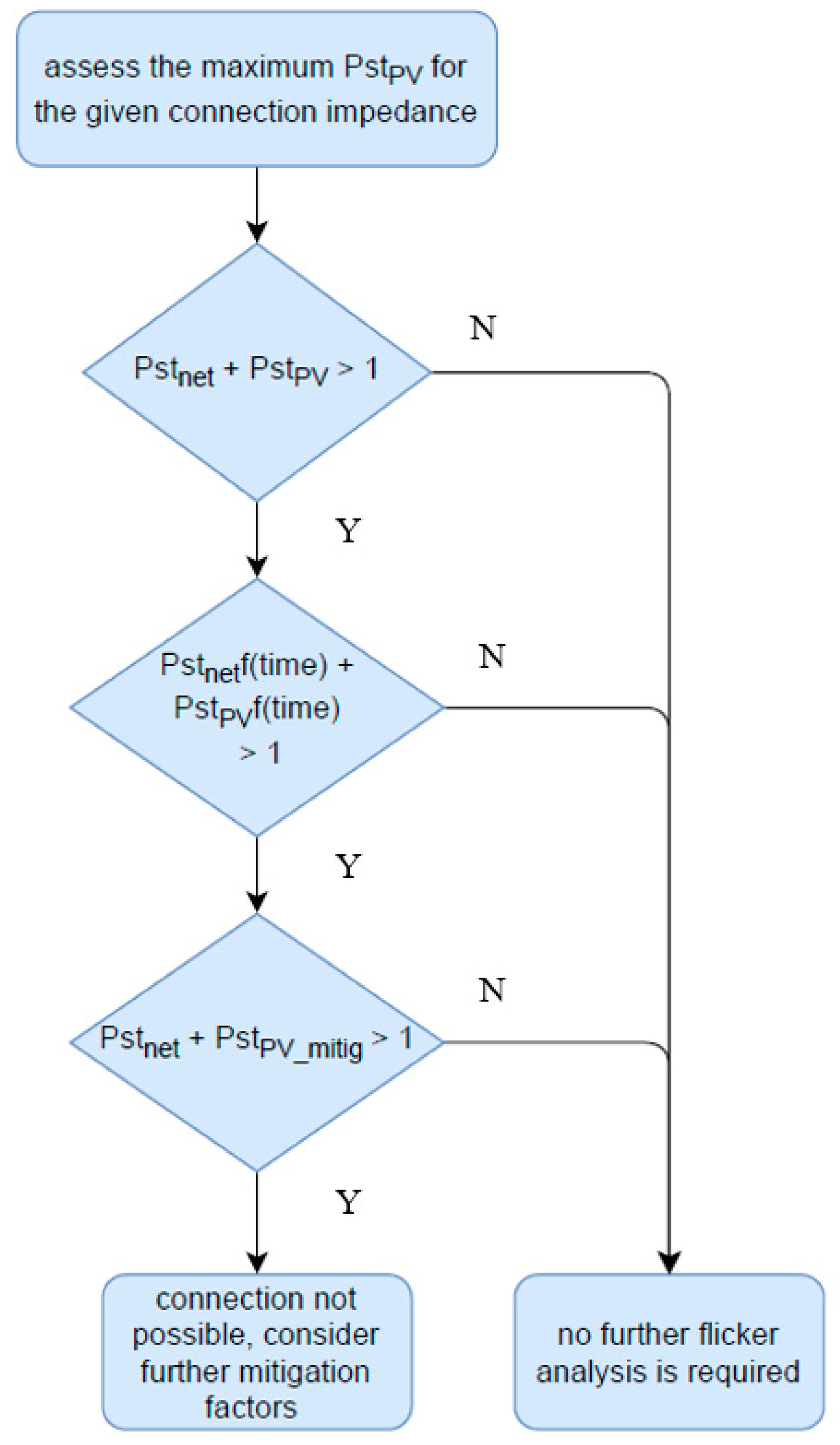
4.3. Procedure of PST Assessment

The presented results are used to develop the methodology of Pst assessment caused by PV sources. The assessment of the PV impact on flicker is presented in Figure 18 starts with an assessment of risk. The initial assessment is based on summing the maximum Pst_1min in the network with the max expected Pst rise (Figure 13; installation B) caused by PV plant, which is assessed based on the most important factor—impedance between PV source and MV/lv transformer. If the sum is lower than the normative threshold, no further analysis is required, and the installation may be safely connected. If, however, the sum is above the threshold, one should perform the more detailed assessment of Pst in order to estimate the risk; a further step involves verification of the probability of Pst rise over the day using PstA and PstB obtained based on Figure 13. If under worst case scenario assumptions, the highest Pst measured in network is increased by the PV source, the probability of Pst rise is within margin defined by standards (exceeding of threshold below 10% of time), and the PV plant could be safely connected. If the condition is not satisfied, further analysis needs to be performed, and one needs to analyze the next factors—the Pst mitigating factors, which are the other PV sources in close vicinity and impact of the background voltage. It is proposed to assess the mitigation factors based on the values presented in the paper; however, different critical values may be defined in order to fulfill local power quality requirements. Finally, if results are inconclusive, one should perform a detailed simulation using the recorded operation of the inverter, which is planned to be installed in a new location. It is believed that long-term measurements obtained in one location could be processed to mimic another type of inverter. However, further analysis is needed. Analyses are also needed in order to verify different flicker measures utilized in different countries, e.g., Arabic countries [33].

5. Summary

In this paper, we present theoretical considerations connected with impact of photovoltaic installations on flicker and voltage fluctuations. Different factors affecting the results are described, among which the most important is impedance between PV source and MV/lv transformer, the power of installation, and distances between installations. Simple method of flicker assessment and verification of the flicker before the connection of PV source with power network is given in order to verify if there is a risk of exceeding the flicker factors defined in the power quality norms, e.g., EN50160.

It is concluded that PV private prosumers installations (<10 kWp) have rather small negative impact on flicker factor and even in some cases can mitigate the flicker level. At the same time, however, the number of slow rate voltage changes is greatly increased after the connection of PV plants, which may cause problems with the voltage regulation and further the active voltage regulation may additionally increase the Pst values. The industrial prosumers (10–40 kWp) can have significant impact on worsening the Pst factors, so in many cases, detailed analysis should be carried out.

Despite the direct impact of PV sources on voltage flicker and fluctuations, one need to consider the indirect impact of PV sources—regulations encourage the prosumers to utilize energy when it is produced. Moreover, in order to utilize the energy excess (more energy is typically produced than used by prosumer), prosumers install new devices, e.g., electrical heating or electric car chargers, etc., which has further negative impact on voltage fluctuations and flicker.

Further research is focused on mitigation of flicker level in distribution system networks.

References

1. Huda, A.N.; Živanović, R. Large-scale integration of distributed generation into distribution networks: Study objectives, review of models and computational tools. Renew. Sustain. Energy Rev. 2017, 76, 974–988. [Google Scholar] [CrossRef]
2. Caamano-Martin, E.; Laukamp, H.; Jäntsch, M.; Erge, T.; Thornycroft, J.; De Moor, H.; Cobben, S.; Suna, D.; Gaiddon, B. Interaction between photovoltaic distributed generation and electricity networks. Prog. Photovolt. Res. Appl. 2008, 16, 629–643. [Google Scholar] [CrossRef]
3. Kacejko, P.; Pijarski, P. Optimal Voltage Control in MV Network with Distributed Generation. Energies 2021, 14, 469. [Google Scholar] [CrossRef]
4. Pijarski, P.; Kacejko, P.; Adamek, S. Analysis of Voltage Conditions in Low Voltage Networks Highly Saturated with Photovoltaic Micro Installations. Acta Energetica 2018, 3, 4–9. [Google Scholar]
5. Zawodniak, J.J.; Łowczowski, K.; Czerniak, M. Connection of PV Sources Into Transmission Grid vs. Thermal Overload Risk of Wires and Cables. Autom. Elektr. Zakłócenia 2021, 13, 48–56. [Google Scholar] [CrossRef]
6. Reno, M.J.; Lave, M.; Quiroz, J.E.; Broderick, R.J. PV ramp rate smoothing using energy storage to mitigate increased voltage regulator tapping. In Proceedings of the 2016 IEEE 43rd Photovoltaic Specialists Conference (PVSC), Portland, OR, USA, 5–10 June 2016. [Google Scholar]
7. Hoff, T.E.; Perez, R. Modeling PV fleet output variability. Sol. Energy 2012, 86, 2177–2189. [Google Scholar] [CrossRef]
8. Chen, X.; Du, Y.; Lim, E.; Wen, H.; Yan, K.; Kirtley, J. Power ramp-rates of utility-scale PV systems under passing clouds: Module-level emulation with cloud shadow modeling. Appl. Energy 2020, 268, 114980. [Google Scholar] [CrossRef]
9. IEEE Power and Energy Society. IEEE 1453—IEEE Recommended Practice for the Analysis of Fluctuating Installations on Power Systems; IEEE: Piscataway, NJ, USA, 2015. [Google Scholar]
10. Pakonen, P.; Hilden, A.; Suntio, T.; Verho, P. Grid-connected PV power plant induced power quality problems—Experimental evidence. In Proceedings of the 2016 18th European Conference on Power Electronics and Applications (EPE’16 ECCE Europe), Karlsruhe, Germany, 5–9 September 2016; pp. 1–10. [Google Scholar] [CrossRef]
11. Lim, Y.S.; Tang, J.H. Experimental study on flicker emissions by photovoltaic systems on highly cloudy region: A case study in Malaysia. Renew. Energy 2014, 64, 61–70. [Google Scholar] [CrossRef]
12. Aziz, T.; Ketjoy, N. PV Penetration Limits in Low Voltage Networks and Voltage Variations. IEEE Access 2017, 5, 16784–16792. [Google Scholar] [CrossRef]
13. Hanzelka, Z. Wahania napięcia. Autom. Elektr. Zakłócenia 2011, 5, 6–22. [Google Scholar]
14. Smart, B.H.P. Power Quality A Guide to Voltage Fluctuation and Light Flicker; BC Hydro: Vancouver, BC, Canada, 2005. [Google Scholar]
15. Musiał, E. Ocena Jakości Energii Elektrycznej w Sieciach Przemysłowych. Autom. Elektr. Zakłócenia 2010, 1, 30–45. [Google Scholar]
16. Hanzelka, Z. Voltage Fluctuations in Power Networks (”Flicker”), EU: European Copper Institute, 2014. Available online: http://leonardo-energy.org/sites/leonardo-energy/files/documents-and-links/cu0208_an_voltage_fluctuations_v1.pdf (accessed on 3 February 2022).
17. Otomański, P.; Wiczyński, G. The usage of voltage and current fluctuation for localization of disturbing loads supplied from power grid. Przegląd Elektrotechniczny 2011, 87, 107–111. [Google Scholar]
18. Commssion, I.E. Electromagnetic Compatibility (EMC)—Part 3: Limits—Section 3: Limitation of Voltage Fluctuations and Flicker in Low Voltage Supply Systems for Equipment with Rated Current ≤16 A; International Electrotechnical Commission: Geneva, Switzerland, 1994. [Google Scholar]
19. Waghmare, S. Induction motor voltage flicker analysis and its mitigation. Int. J. Eng. Sci. Technol. 2010, 2, 7626–7640. [Google Scholar]
20. Kot, A.; Szpyra, W. Optymalna regulacja napięcia w sieciach rozdzielczych średniego napięcia. Acta Energetica 2009, 2, 89–105. [Google Scholar]
21. Chmura i Partnerzy Radcowie Prawni Sp. p., Rozliczenia Prosumentów w Latach 2022–2024 (Fotowoltaika, Odnawialne źródła Energii). Co się Zmieni? Od kiedy? January 2022. Available online: https://www.infor.pl/prawo/nowosci-prawne/5393258,Rozliczenia-prosumentow-w-latach-20222024-fotowoltaika-odnawialne-zrodla-energii-Co-sie-zmieni-Od-kiedy.html (accessed on 9 February 2022).
22. Bhattacharyya, S.; Cobben, S.; Myrzik, J.; Kling, W. Flicker propagation and emission coordination study in a simulated low voltage network. Eur. Trans. Electr. Power 2010, 20, 52–67. [Google Scholar] [CrossRef]
23. Rozehna, P.; Krejčí, P. Power quality complaints and monitoring of flicker in selected area s of northern Moravia. In Proceedings of the 18th International Scientific Conference on Electric Power Engineering (EPE), Kouty nad Desnou, Czech Republic, 17–19 May 2017. [Google Scholar]
24. Bhattacharyya, S.; Cai, R.; Cobben, S.; Myrzik, J.; Kling, W. Flicker propagation study in a typical Dutch grid. In Proceedings of the CIRED 2009—20th International Conference and Exhibition on Electricity Distribution-Part 1, Prague, Czech Republic, 8–11 June 2009; p. 102. [Google Scholar] [CrossRef] [Green Version]
25. Chmielowiec, K.; Kuwałek, P.; Wiczyński, G. Zastosowanie Liczników AMI do Oceny Jakości Energii Elektrycznej; PTPiREE: Poznań, Poland, 2020. [Google Scholar]
26. Mandelli, S.; Merlo, M.; Colombo, E. Novel procedure to formulate load profiles for off-grid rural areas. Energy Sustain. Dev. 2016, 31, 130–142. [Google Scholar] [CrossRef]
27. Elspec, Pure BlackBox. Available online: https://www.elspec-ltd.com/metering-protection/power-quality-analyzers/purebb-power-quality-analyzer-handheld/ (accessed on 9 February 2022).
28. IEEE. IEEE 929-2000 Recommended Practice for Utility Interface of Photovoltaic (PV) Systems. 0.1109/IEEESTD.2000.91304; IEEE: Piscataway, NJ, USA, 2000. [Google Scholar]
29. Inzunza, R.; Tawada, Y.; Furukawa, M.; Shibata, N.; Sumiya, T.; Tanaka, T.; Kinoshita, M. ∆r of a Photovoltaic Inverter Under Sudden Increase in Irradiance due to Reflection in Clouds. In Proceedings of the 4th International Conference on Renewable Energy Research and Applications, Palermo, Italy, 22–25 November 2015. [Google Scholar]
30. Olex, Catalogue—Aerial. Available online: https://www.se.com/ww/library/SCHNEIDER_ELECTRIC/SE_LOCAL/APS/212274_DC2A/Olex_cables.pdf (accessed on 25 February 2022).
31. Yang, X.; Kratz, M. Power System Flicker Analysis by RMS Voltage Values and Numeric Flicker Meter Emulation. IEEE Trans. Power Deliv. 2009, 24, 1310–1318. [Google Scholar] [CrossRef]
32. PV Monitor. Available online: https://pvmonitor.pl/index.php (accessed on 24 February 2022).
33. Wiczyński, G. Porównanie miar wahań napięcia. Pozn. Univ. Uf Technol. Acad. J. 2012, 72, 9–16. [Google Scholar]
Figure 1. Vector diagram presenting voltage drop in circuit with series RL impedance.
Energies 15 02075 g001
Figure 2. Flicker severity in The Netherlands (2007), adapted from [22,24].
Energies 15 02075 g002
Figure 3. Output power during the exemplary day.
Energies 15 02075 g003
Figure 4. Strat-up of inverter A (orange—active power; blue—reactive power).
Energies 15 02075 g004
Figure 5. Strat-up of inverter B (orange — active power; blue — reactive power).
Energies 15 02075 g005
Figure 6. Model of LV network; lv feeder made of 4 × 70 insulated aerial bundle (R1 = 0.443 Ω/km and X1 = 0.088 Ω/km) and consumer line made of 4 × 16 YAKY cable (R1 = 1.19 Ω/km, X1 = 0.092 Ω/km); parameters of lines based on [30].
Energies 15 02075 g006
Figure 7. Impact of utility line length (4 × 70) on max PST and share of Pst1min above 0.03.
Energies 15 02075 g007
Figure 8. Output power of inverter B during highly variable shadow conditions 17.03.
Energies 15 02075 g008
Figure 9. Impact of number of 10 kVA PV inverters on Pst1min.
Energies 15 02075 g009
Figure 10. Predicted flicker emitted by industrial-scale PV sources.
Energies 15 02075 g010
Figure 11. Output profiles of 2 PV sources located approximately 100 m away from each other; based on data [32].
Energies 15 02075 g011
Figure 12. Impact of distance between two PV sources on Pst in PCC of two PV plants Pst1min.
Energies 15 02075 g012
Figure 13. Impact of daytime on Pst factor; A—average over 3 months for installation A connected to 250 m utility cable 4 × 70; B—average over 1 month for installation B connected to 250 m utility cable.
Energies 15 02075 g013
Figure 14. Pst trend installation B 250 m 1 min.
Energies 15 02075 g014
Figure 15. Impact of voltage profiles recorded in suburban areas (based on the fragment of profile from 17.03, installation B); one PV source, two PV sources, three PV sources (assuming instantaneous power variations).
Energies 15 02075 g015aEnergies 15 02075 g015b
Figure 16. Impact of different voltage profiles—blue—urban, green—suburban; red—mixed on Pst1min (based on profile of installation B form 17.03).
Energies 15 02075 g016
Figure 17. The impact of voltage profile on 2% voltage change caused by PV source (inverter B, profile from 17.03—Figure 8) 1—urban, 2—suburban, 3—mixed, 4—all results combined; blue—500, green—750, and red—1000 m utility 4 × 70 line.
Energies 15 02075 g017
Figure 18. PV assessment flowchart.
Energies 15 02075 g018