Article

Modelling of Boil-Off and Sloshing Relevant to Future Liquid Hydrogen Carriers

by
Jessie R. Smith
1,*,
Savvas Gkantonas
1 and
Epaminondas Mastorakos
1,2
1
Department of Engineering, University of Cambridge, Cambridge CB2 1PZ, UK
2
Cambridge Centre for Advanced Research and Education in Singapore (CARES), Singapore 138602, Singapore
*
Author to whom correspondence should be addressed.
Energies 2022, 15(6), 2046; https://doi.org/10.3390/en15062046
Submission received: 7 February 2022 / Revised: 3 March 2022 / Accepted: 5 March 2022 / Published: 10 March 2022
(This article belongs to the Special Issue Energy-Saving and Carbon-Neutral Technologies for Maritime Transport)

Abstract

:
This study presents an approach for estimating fuel boil-off behaviour in cryogenic energy carrier ships, such as future liquid hydrogen (LH2) carriers. By relying on thermodynamic modelling and empirical formulas for ship motion and propulsion, the approach can be used to investigate boil-off as a function of tank properties, weather conditions, and operating velocities during a laden voyage. The model is first calibrated against data from a liquefied natural gas (LNG) carrier and is consequently used to investigate various design configurations of an LH2 ship. Results indicate that an LH2 ship with the same tank volume and glass wool insulation thickness as a conventional LNG carrier stores 40% of the fuel energy and is characterised by a boil-off rate nine times higher and twice as sensitive to sloshing. Adding a reliquefaction unit can reduce the LH2 fuel depletion rate by at least 38.7% but can increase its variability regarding velocity and weather conditions. In calm weather, LH2 boil-off rates can only meet LNG carrier standards by utilising at least 6.6 times the insulation thickness. By adopting fuel cell propulsion in an LH2 ship, a 1.1% increase in fuel delivery is expected. An LH2 ship with fuel cells and reliquefaction is required to be at least 1.7 times larger than an existing LNG carrier to deliver the same energy. Further comparison of alternative scenarios indicates that LH2 carriers necessitate significant redesigns if LNG carrier standards are desired. The present approach can assist future feasibility studies featuring other vessels and propulsion technologies, and can be seen as an extendable framework that can predict boil-off in real-time.

Graphical Abstract

1. Introduction

Traditionally, energy carrier ships transport fossil fuels over long distances for utilisation in locations far from their origin [1]. However, the current global drive to limit greenhouse gas emissions has led to a search for low-carbon energy transport carriers propelled by low-carbon fuel. The use of cryogenic liquid low-carbon fuels for these purposes could significantly decarbonise the shipping industry and increase the capacity for transportation of low-carbon energy stores [2]. Due to their low temperatures, cryogenic liquids gradually boil off throughout a voyage [3]. The boiled-off gas (BOG) can be used to propel a ship [4], but it has to be of the right quantity to avoid losing excess gas to the atmosphere or passing it through costly reliquefaction systems [5]. Sloshing, i.e., fluid movement induced by ship motion increases BOG generation by (i) transferring heat to the tank system in the form of dissipated kinetic energy and (ii) increasing the surface area between the liquid and vapour phases [6]. As a result, the final fuel boil-off rate (BOR) is sensitive to tank design, ship operation, and weather conditions and needs to be carefully considered to minimise cost and energy losses in current and future cryogenic fuel carriers.
Two examples of cryogenic liquid fuels are liquified natural gas (LNG) and liquid hydrogen (LH2) [7]. On the one hand, LNG is commonly transported by and used to propel energy carrier ships [8], with LNG ships having a lower carbon dioxide (CO2) equivalent emission due to propulsion than conventional oil-powered ships [9]. These ships cannot be carbon-neutral unless the CO2 is captured during the voyage [10]. To make matters worse, the methane contained in the BOG can have 25 times the warming effect of CO2 if released directly into the atmosphere [11]. On the other hand, an LH2 ship does not contribute any significant greenhouse gas emissions during its voyage. LH2 ships can also result in lower overall CO2 equivalent emissions than LNG ships (depending on the fuel source), showing excellent carbon neutrality potential [7]. Given the compelling nature of hydrogen, the construction of LH2 carriers is of vital importance for future decarbonization strategies, and their design can benefit from existing knowledge on LNG ships. However, the boiling point of LH2 is around 90 °C less than that of LNG, raising several technical challenges since BOR effects on LH2 can be more pronounced and more insulation and reliquefaction infrastructure is required to contain the fuel [12,13,14].
Relative to LNG carriers, LH2 carrier design is still in the development stages, so design specifications are not well established. While the largest existing LNG ships can carry 265,000 m3 of fuel [15], the only existing LH2 carrier ship (the Suiso Frontier) transports 1250 m3 at a time. This ship employs one horizontal, cylindrical, vacuum-insulated tank and utilises a hybrid natural gas and hydrogen turbine for propulsion [16]. A working LH2 carrier has also recently been commissioned with a volumetric capacity of the order of an LNG ship: it will transport 160,000 m3 of LH2 in 4 spherical vacuum-insulated tanks [17,18]. Other variants of conceptual LH2 ships that employ several forms of propulsion are still under investigation. For example, future LH2 ships may be propelled by hydrogen combustion using reciprocating engines [19] or combined-cycle gas turbines [19,20]. Alternatively, ships may employ electric propulsion with fuel cells using proton exchange membrane (PEM) [21,22,23,24], solid oxide [22], or molten carbide [19] technology. The possibility of including a reliquefaction unit on these ships also exists, as discussed by Ahn et al. [19].
In conceptual LH2 ship studies, LH2 is assumed to be stored either in prismatic (type A) containers [19,24], spherical (type B) containers [14], or cylindrical (type C) containers [20,23,25,26]. The storage tanks are insulated by vacuum casing [19] or a low-conductivity material such as Polyurethane Foam [20]. The required thickness of insulation is not widely reported. In Alkhaledi et al. [20], it is assumed that 1 m of Polyurethane Foam is required to insulate the tank appropriately. In contrast, a recent whitepaper examining the sustainability of hydrogen as a fuel for shipping estimates that two to three times the insulation of a conventional LNG tank is required to appropriately insulate LH2 (equivalent to 1 to 1.6 m of low-conductivity material insulation) [27,28]. As far as BOR in LH2 tanks is concerned, only three conceptual LH2 ship investigations attempt its prediction [14,19,29]. Either experimental observations [29] or thermodynamic models [14,19] are used to relate the heat transfer coefficient through the tank walls to the BOR. In particular, Al-Breiki et al. [14] compared the BOR properties of LH2 and other low-carbon fuels to LNG showing that an LH2 ship has a BOR of 1.063%/day while a similar LNG ship has a much lower BOR of 0.1204%/day. The studies of References [14,19,29] relate the BOR of LH2 to a specific ship design; however, none investigate the impact of ship design on BOR or vice versa.
The thermodynamic effects of sloshing in LH2 ships are also not widely investigated. Maekawa et al. (2017) [30] and Maekawa et al. (2018) [31] observed liquid level and temperature measurements for 0.02 m3 of LH2 in a test ship subjected to manoeuvre-induced sloshing in several planes of motion. Wei et al. [32] further investigated sloshing-induced pressure changes in the specific case of a tank filled with LH2. Other cryogenic fluids have been studied more closely. For example, Behruzi et al. [33] and Grotle and Aesoy [34] modelled pressure and temperature changes in sealed LNG tanks that result from sloshing at various excitation frequencies and amplitudes. In some cases, thermodynamic changes can also be related to BOG generation during a ship voyage, as in Wu and Ju [35]. In other cases, the BOR in unsealed tanks can be directly investigated at various slosh excitations as in Yu et al. [36] and Mir et al. [37]. In addition, Ludwig et al. [38] derived a relationship between sloshing frequency, sloshing amplitude, and heat transfer rate across the liquid-vapour interface, general enough to apply to any cryogenic fuel. For modelling purposes, the sloshing-induced heat transfer is of special interest; hence it must be considered in any thermodynamic modelling approach focusing on the BOR.
The external weather conditions and ship operation, including cruising speed and manoeuvring that can cause intense sloshing, have been the subject of many investigations as they are essential for any cargo type, including cryogenic fuels [39,40]. However, the resultant BOR of LH2 has never been studied in this context, with data being available primarily for LNG. For example, Jeong et al. [41] present a model that suggests routing and operating velocities for an LNG ship voyage to minimise fuel depletion. Although the BOR and fuel utilisation rate are estimated, sloshing effects are not considered in this study. Simple empirical relationships that directly relate weather parameters to thermodynamic properties can be derived and used to calculate BOR due to sloshing along a voyage with a non-constant ship velocity [6]. More detailed models linking the ship’s coupled motion with fluid movement in the tank are also available [42] but have not yet been coupled with thermodynamic models due to their complexity.
This paper introduces an approach that predicts the natural and sloshing induced BOR properties of cryogenic energy carrier ships, and considers various practical implications relevant to the tank properties, weather conditions, and operating velocities during a laden voyage. Any cryogenic liquid can be modelled, but a conceptual LH2 ship is selected here, given its potential for decarbonization and the associated design problems that may arise due to BOR. As a demonstration, the conceptual LH2 ship is based on the standards of a conventional LNG ship with a 173,600 m3 capacity, for which data are available. The approach is then employed to explore the effects of (i) weather conditions, (ii) operating velocity, (iii) sloshing, and (iv) ship design on the BOR properties of a conceptual LH2 ship.
The approach integrates existing relationships from a range of areas in the literature such as thermodynamics, ship power consumption, ship motion in rough seas, and sloshing in cryogenic tanks. As discussed above, several of these areas lack sufficient scrutiny, meaning that the relationships employed are often not well established, and data (experimental or otherwise) is insufficient to conduct an in-depth evaluation of the model. However, the merit of the current approach is its novelty for estimating the BOR and final fuel delivery of conceptual LH2 ships directly from voyage weather conditions. The overall modelling framework is amenable to updates as more data becomes available, with all sub-models and governing equations being consolidated in a Python-based interface named Chione.
The remainder of the paper is as follows. First, the thermodynamic equations for a cryogenic tank, including boil-off and sloshing, are detailed. Next, the ship model is outlined: the sizing of the ship, its power consumption, and the relationship between ship velocity, weather conditions, and sloshing are explored. The approach is then calibrated using data from a conventional LNG ship, conceptual studies on LH2 ships, reliquefaction units, and electric component data. This is followed by an investigation of the suitability of using LH2 ships as fuel carriers, focusing on the effects of insulation thickness, the presence or absence of reliquefaction, and propulsion type. Finally, conclusions and recommendations for future work close the paper.

2. Thermodynamic Model

2.1. Generalised Thermodynamic Model

A representation of the liquid and vapour control volumes in the fuel tanks is shown in Figure 1. The control volumes are annotated with symbols representing relevant properties of the liquid and vapour phases and heat, mass, and enthalpy transfer rates to and from them. This approach is similar to those presented in Al Ghafri et al. and Petitpas et al. [29,43]. In this study, however, the tanks are unsealed, so the internal tank pressure is assumed to be constant. The application of the First Law of Thermodynamics to the vapour control volume results in:
Q ˙ V Q ˙ V , if + ( m ˙ L m ˙ V ) × h V = U ˙ V ,
where
U ˙ V = ( m ˙ L m ˙ V ) × u V + m V × T ˙ V × du V / dT V ,
with h V representing the specific enthalpy of the vapour. Likewise, by applying the First Law of Thermodynamics to the liquid control volume, Equations (3) and (4) are derived:
Q ˙ L + Q ˙ if , L m ˙ L × h L = U ˙ L ,
where
U ˙ L = m ˙ L × u L + m L × T ˙ L × u L / T L ,
with h L being the specific enthalpy of the liquid.
The heat transfer rate across the walls into the liquid ( Q ˙ L ) and vapour ( Q ˙ V ) are functions of the temperature difference between the external environment ( T out ) and the liquid ( T L ), and vapour ( T V ) as well as the surface area of heat transfer and the heat-transfer coefficient through the tank walls ( U ins ). It is evident from Equations (2) and (4) that the rate of change of internal energy of the liquid ( U ˙ L ) and vapour ( U ˙ V ) are functions of the specific internal energy of the liquid ( u L ) and vapour ( u V ). In turn, these variables are functions of the liquid and vapour temperatures and are here calculated using Cantera [44]. The variables U ˙ L and U ˙ V are also functions of the mass of liquid ( m L ) and vapour ( m V ), the mass flow rates out of the liquid ( m ˙ L ) and vapour ( m ˙ V ), and the rates of change of the liquid ( T ˙ L ) and vapour ( T ˙ V ) temperatures.
A control surface representing the liquid-vapour interface is also shown in Figure 1. The control surface is used to define the heat transfer rates from the vapour to the interface ( Q ˙ V , if ) and from the interface to the liquid ( Q ˙ if , L ) in Equations (1) and (3). The surface is treated similarly to the liquid and vapour control volumes, but it has no mass. The interface is assumed to be the site of boil-off within the tanks, so its temperature is assumed to be that of the saturated cryogenic fluid ( T sat ). Thus Equation (5) represents the First Law of Thermodynamics for the liquid-vapour control surface:
Q ˙ V , if Q ˙ if , L + m ˙ L × ( h L h V ) = 0 .
The kinetic energy transfer rate to the tank due to sloshing ( W ˙ slosh ) acts to increase the BOR, so this term can be modelled to act at the interface control surface. However, the kinetic energy term is negligible relative to the heat transfer rates through the interface. Therefore, it is not included in Equation (5), and sloshing is assumed to act only in the context of increasing the heat transfer rate across the liquid-vapour interface. Q ˙ V , if introduces sloshing to the thermodynamic model, as in Equation (6):
Q ˙ V , if = SSF × U if × A if × ( T V T sat ) ,
where A if represents the surface area of the interface. The heat transfer coefficient across the interface is separated into two independent variables: U if and SSF. The variable U if represents the heat-transfer coefficient across the interface in the absence of sloshing. The Sloshing Scaling Factor (SSF, dimensionless) is the degree by which heat transfer across the interface increases with the sloshing of the cryogenic fuel. It is dependent on the velocity of the ship and the external weather conditions.

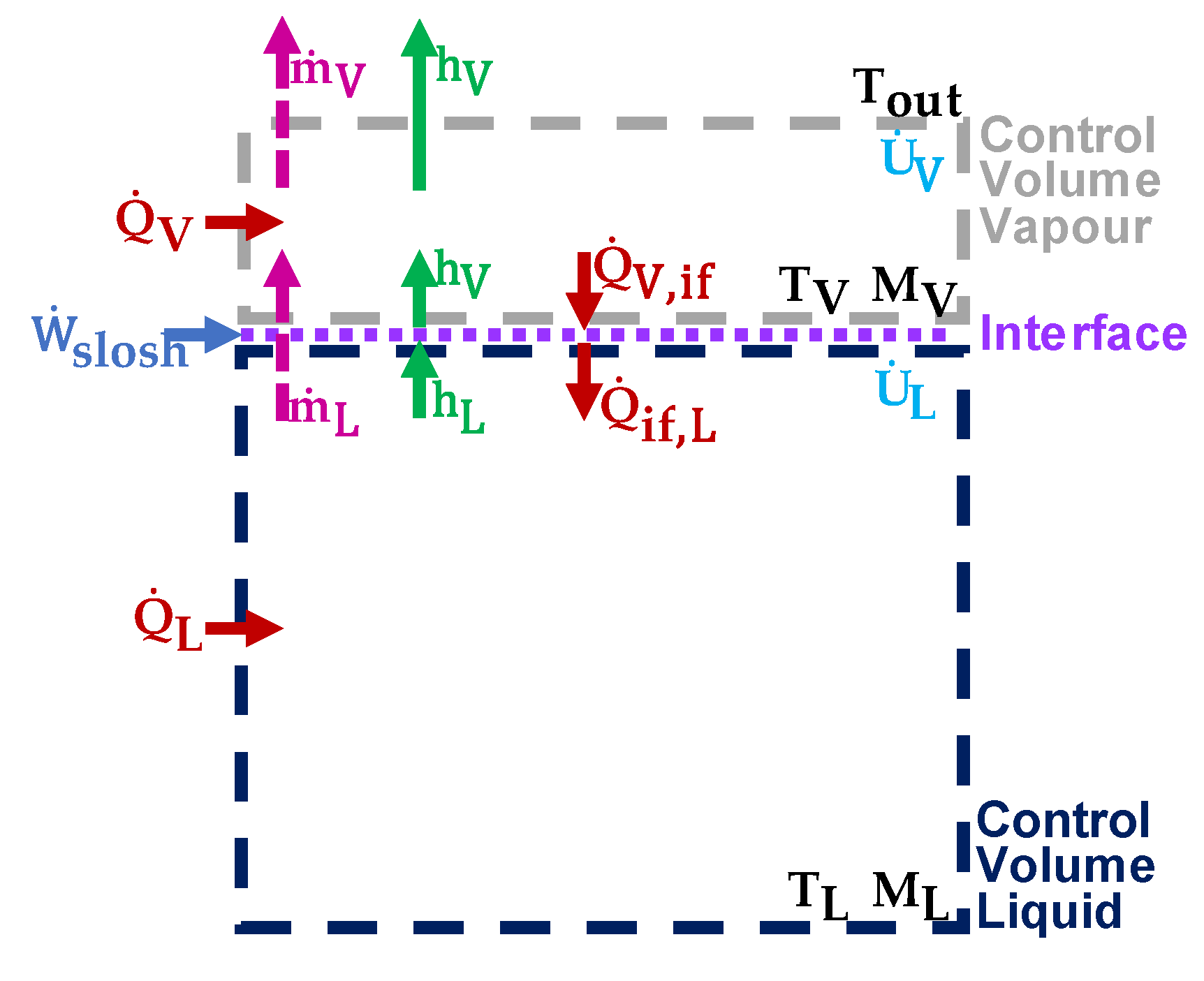
2.2. Thermodynamic Model for an Unsealed, Laden Cryogenic Tank

The thermodynamic model of the fuel tanks in Section 2.1 is general but can be simplified by defining the fuel tanks as unsealed and laden. In an unsealed tank, the BOG is vented, so the pressure remains constant instead of rising as the BOG accumulates. The ship tank carries a high proportion of liquefied fuel during a laden voyage, with only a small volume of fuel vapour on top of the liquid. Qu et al. [6] models an unsealed LNG carrier subjected to sloshing and is undertaking a laden voyage and shows that liquid and vapour temperature measurements display only minor variations over several days. In the present study, the liquid and vapour temperatures are thus modelled as constants over time. An approximately constant liquid temperature is also consistent with observations by Krikkis et al. [4]; however, a constant vapour temperature was not observed as the vapour fraction during the laden voyage is significantly higher than that modelled here. Since the pressure and temperature of the liquid and vapour are assumed constant over time, the vapour mass must also be considered constant. Hence, the fuel evaporation rate (or m ˙ L ) is assumed equal to the total BOR from the tanks (or m ˙ V ) based on mass conservation.
Furthermore, by applying the unsealed and laden assumptions to Equation (1), it is evident that there is no net enthalpy transfer into and out of the vapour and no net change in internal energy. The vapour thus acts as an extra insulating layer on top of the liquefied fuel. The heat transfer rate into the layer is equal to the heat transfer rate out, as in Equation (7):
Q ˙ V = Q ˙ V , if
The vapour temperature can thus be related directly to the surface areas and heat-transfer coefficients across the wall and the interface, as in Equation (8):
( T out T V ) / ( T V T sat ) = SSF × ( U if / U ins ) × ( A if / A V , in ) ,
where A V , in (m2) is the surface area of heat transfer across the tank walls to the vapour.
By summing the governing equations for the vapour, liquid, and their interface (Equations (1), (3), and (5)), an expression can be derived for the whole tank. The assumptions outlined above may also be applied to simplify the expression further, as in:
m ˙ use + m ˙ loss total   BOR = ( Q ˙ L + Q ˙ V ) / ( h V u L ) .
Without reliquefaction, the total BOR can be expressed as the sum of the fuel loss rate to the atmosphere ( m ˙ loss ) and the fuel utilisation rate in the engine ( m ˙ use ). The value of m ˙ use is determined from the power requirements of the ship, so Equation (9) can also be expressed in terms of m ˙ loss .
Equations (8) and (9) form the system of thermodynamic equations used to determine the BOR from the external weather conditions and the ship′s velocity. The heat transfer coefficients and the surface area of the tank walls can be determined from empirical data of the tank properties. For a design BOR and fuel temperature, Equation (8) can be solved to determine the temperature of vapour, and then Equation (9) can be utilised to determine U if . This process will be demonstrated in the following sections using data for a 173,600 m3 capacity LNG carrier. U if is, by definition, independent of any changes caused by sloshing. Thus, for any SSF value around the design point, a corresponding temperature of vapour, hence BOR, can again be determined using Equations (8) and (9). The dependency of SSF on external weather conditions and ship velocity may also be defined using existing data and relationships from the literature, as will be shown later.

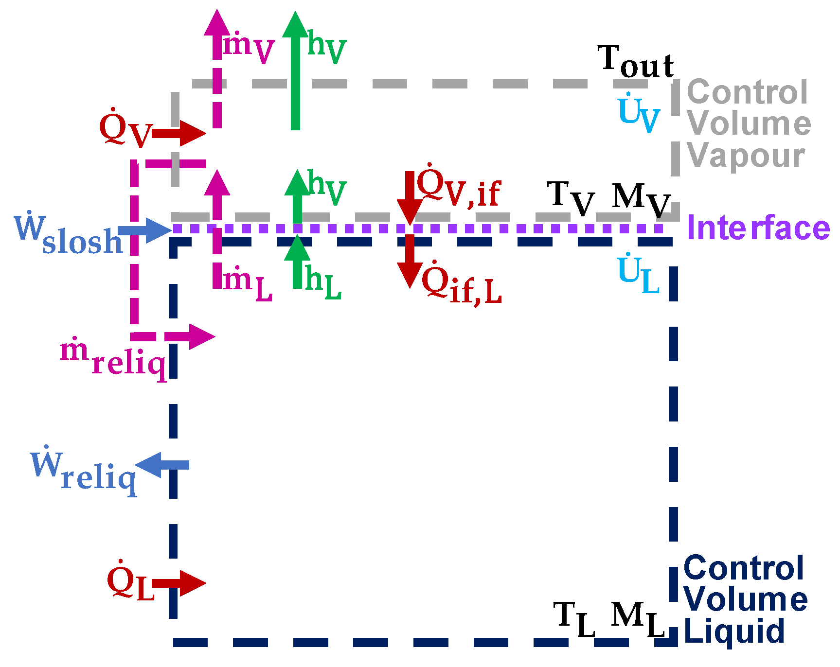
2.3. Addition of a Reliquefaction Unit

The reliquefaction process considered in this study is based on a reverse Brayton cycle [45,46,47,48]. When reliquefaction is employed, the unutilised BOG is recycled back to the tank, with some additional fuel consumed to generate electricity for the work needed to drive the reliquefaction process. In place of Figure 1, Figure 2 represents the liquid and vapour control volumes in such a ship. By applying the First Law of Thermodynamics to the vapour, Equation (1) is replaced with:
Q ˙ V Q ˙ V , if + ( m ˙ L m ˙ V m ˙ reliq ) × h V = U ˙ V ,
where m ˙ reliq (kg s−1) represents the rate of fuel reliquefaction. Likewise, Equation (3) for the liquid is replaced with:
Q ˙ L + Q ˙ if , L W ˙ reliq + m ˙ reliq × h V m ˙ L × h L = U ˙ L ,
where W ˙ reliq (W) is the enthalpy extraction rate during the reliquefaction process. This quantity can be expressed in terms of the rate of fuel reliquefaction as in:
W ˙ reliq = m ˙ reliq × ( h V h L ) .
All assumptions made in Section 2.2 that are associated with the tank being unsealed and laden also apply here. It is thus assumed that the liquid and vapour temperatures are constant, and the mass flow rates into and out of the vapour sum to zero. By summing Equations (5), (10), and (11), Equation (9) can then be replaced with:
m ˙ use + m ˙ r - use total   fuel   depletion   rate = ( Q ˙ L + Q ˙ V W ˙ reliq ) / ( h V u L ) ,
which provides an expression for the whole tank with reliquefaction.
It is assumed that all unutilised boil-off gas is reliquefied as m ˙ reliq so that the term m ˙ loss is small enough to be negligible. Thus, the fuel depletion rate from the tank can be expressed as the sum of the fuel utilisation rates for propulsion ( m ˙ use ) and reliquefaction ( m ˙ r - use ). While the fuel utilisation rate for propulsion is dependent only on the ship power requirements, the fuel utilisation rate for reliquefaction is also dependent on the electricity requirements of reliquefaction and the rate of fuel reliquefaction ( m ˙ reliq ).
Equation (8) can be combined with Equation (13) to form a system of equations that can be solved to find the fuel depletion rate at different ship velocities and weather conditions. As in the tank model without reliquefaction, data from an LNG ship will be used in the following sections to find U if in the case with reliquefaction, which can, in turn, be used to find the fuel depletion rate at different values of SSF. Note that the independent variable in Equation (13) is m ˙ reliq , as opposed to m ˙ loss used in Equation (9) .

3. Ship Model

3.1. Ship Sizing

It is assumed that stored energy in the cryogenic fuel is converted into ship motion by reciprocating internal combustion (IC) engines, or else Proton Exchange Membrane (PEM) fuel cells and electric motors, using BOG. Some BOG may also be lost to the atmosphere unless reliquefaction is included. The cryogenic ship propelled by combustion is modelled to consist of fuel (in both liquid and vapour phase), IC engines, fuel tanks, ballast water, and extra volume that is not accounted for by any of the former components (referred to as unassigned volume). Onboard a ship that employs electric propulsion, the IC engines are substituted for fuel cells and electric motors.
In a ship that employs reliquefaction, the unutilised BOG is reliquefied and fed back into the fuel tank as a liquid. A reliquefaction unit, powered by electricity, performs this function. Therefore, two extra components are required onboard combustion ships: a reliquefaction unit and a generator. A generator is not required onboard electric ships that employ reliquefaction; instead, electricity from the PEM fuel cells is used to power the reliquefaction unit.

3.2. Power Consumption and Fuel Utilisation
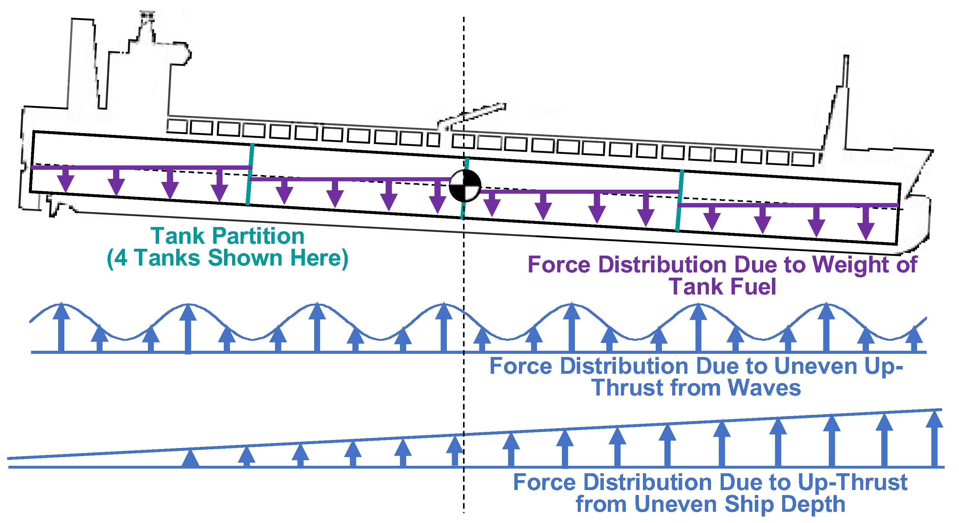
The power consumption of the cryogenic ship ( P use ), is estimated using Equation (14), which is derived from formulas in Molland et al. and Chi et al. [49,50], as in:
P use = c use × A wet × ρ sea × PF × f
Using an equation for LNG carriers in Moser et al. [51], the wetted surface area, A wet , is estimated from the ship deadweight. The power factor ( PF , dimensionless) is a function of the Beaufort number ( BN ). The velocity function ( f , dimensionless) is dependent on the velocity of the ship relative to a fixed point ( v ship ). Formulae that describe the power factor and velocity function are expressed as follows:
PF = ( 1 + 0.005 × BN + BN 6.5 / ( 270 × ( M dead / ρ sea ) 2 / 3 ) ) 3 ,
f = v ship 3 / ( log 10 Re sea 2 ) 2 ,
where M dead is the ship deadweight and ρ sea is the density of sea water. In Equation (16), the Reynolds number ( Re sea ), is based on the ship’s length and uses sea water as a working fluid with properties detailed in Table A1 in Appendix A.
The fuel utilisation rate of the ship makes up part of the total BOR or fuel depletion rate (Section 2.2 and Section 2.3). It is calculated from the power consumption as in:
m ˙ use = P use / ( η eng × η FC × LCV ) ,
where LCV (J kg−1) is the lower calorific value of the fuel. The unknowns in Equations (14)–(17) are the power consumption calibration factor ( c use , dimensionless), the efficiency of fuel cells ( η FC ) if present (if not, η FC = 1 ), and the efficiency of the ship IC engines or electric motors ( η eng ). For combustion ships, the unknown values can be determined by scaling them to match empirical data on power, fuel utilisation rate, and velocity. This is further discussed using data for an existing LNG carrier. For electric ships, η eng and η FC may be found from the literature (e.g., see References [52,53,54,55]).
Onboard a ship that employs reliquefaction, extra fuel must be utilised to reliquefy the unutilised BOG, as demonstrated by:
M ˙ r - use = e reliq × m ˙ reliq / ( η eng × η FC × η gen × LCV ) .
The required fuel utilisation rate ( m ˙ r - use ) is dependent on the mass flow rate of fuel to be liquefied (determined as in Section 2.3) and the electrical energy required per unit mass of reliquefied fuel ( e reliq ). It is also dependent on the efficiency of the generator ( η gen , dimensionless) onboard combustion ships (on electric ships η gen = 1 ). The value of e reliq is dependent on the cryogenic fuel undergoing reliquefaction; due to its lower boiling point, LH2 requires more energy to reliquefy than LNG. Its value and the value of η gen can be determined from the literature (e.g., References [45,46,47,48,56,57]).

3.3. Sloshing

Waves at the liquid-vapour interface of the fuel are produced as a result of sea waves that cause the ship to tilt. This fuel wave enhances heat transfer between the liquid and vapour. Figure 3 represents a cryogenic fuel carrier tilting due to the uneven distribution of waves around its centre of mass. Here, we provide a method of deriving the amplitude and frequency of the fuel wave and the subsequent enhancement of heat transfer for a range of weather conditions and ship velocities. It should be noted that more precise physical descriptions of this relationship are either complex or specific to conditions the ship is travelling in. Given the lack of data for calibration, and for the sake of simplicity, we herein focus only on simplified relationships that demonstrate the effects of the external conditions on sloshing and, by extension, sloshing-induced heat transfer. The model is constructed so that, in future work, these equations may be updated or substituted to improve reliability. For example, sloshing responses of the ship may be determined with more accuracy by utilizing ship accelerometer data to obtain response amplitude operators [39].
Figure 4a–c shows the velocities, amplitudes, and frequencies used to calculate the sea and fuel wave properties. These quantities are shown at Beaufort numbers (BN) of 0 to 12, a value which we use to quantify the weather conditions through which the ship is travelling. To determine the frequency and amplitude of the waves, the velocity of the sea ( v sea ) and ship ( v ship ) must first be determined. Figure 4a details all velocities involved in this calculation. For each BN, the variable ship velocity is shown at its maximum value, assumed to be the velocity at which the ship engines operate at their rated power. The ship velocity relative to a fixed point and to the sea are shown. As a worst-case scenario, the velocity of the sea is assumed to act opposite to the ship’s progress. This assumption is not applicable under many circumstances as the relative direction of ship and sea velocities are specific to the voyage.
The velocity of the sea is determined from the mid-range value of wind velocity ( v wind ), which is found from raw data ranges detailed in tables relating BN to weather conditions [58]. The relationship between wind velocity and sea velocity is found by correlating data in Xue and Chai [59]. The resulting relationship can be expressed by:
v sea = 0.1179 × v wind 0.2528 ,
which is based on sample data specific to location and weather conditions. As a result, it may not apply to all voyages. By directly applying a voyages’ sea speed and direction data, the model presented in this study could instead be utilised to predict sloshing characteristics specific to the voyage in question.
The frequencies of the sea and fuel waves are shown in Figure 4b. Both waves are assumed sinusoidal. The external sea waves are assumed to have a natural frequency of a gravity wave ( ω sea ), given by:
ω sea = 2 π × g / D sea ,
where D sea represents the amplitude of the sea wave and g the acceleration due to gravity. Like v wind , the amplitude of sea waves shown in Figure 4c is obtained from raw data that relate BN to weather conditions [58]. The breaking of sea waves occurs between BN = 7 and BN = 9, and there is little variation in sea wave amplitude within this range [60]. The frequency of the fuel waves is assumed to be equal to the frequency of the sea waves, scaled by the ratio of the resultant velocity of the ship and the velocity of the sea. At a ship velocity of zero, the frequency of the fuel wave is thus equal to the frequency of the sea wave.
The amplitude of the fuel waves shown in Figure 4c is determined by considering a balance of moments acting on the centre of mass of the ship. A representation of the force distributions acting on the ship is detailed in Figure 3. There are three force distributions included in the balance of moments: (i) an uneven hydrostatic force distribution due to the tilt of the ship, (ii) a hydrostatic force distribution due to the uneven distribution of sea waves, and (iii) the uneven weight distribution of fuel. The fuel wave amplitude is assumed to be the height that the fuel rises to keep its surface level within the tilting tanks. This height is low relative to the length of the ship, so it is approximated as half the length of one tank multiplied by the tilting angle of the ship. In the case presented here, the ship′s hull is assumed to be rectangular. The tilting hydrostatic force and fuel weight distributions are dependent on the tilt angle of the ship, so the moment balance allows this angle and the fuel amplitude to be obtained. As the ballast water is present to stabilise the ship, it is assumed that its weight imparts no net moment.
Given fuel wave amplitude and frequency knowledge, the sloshing-induced heat transfer rate enhancement can then be approximated based on Ludwig et al. [38]. In particular, the dependence of SSF (appearing in Equations (6) and (8)) may be given by:
SSF = 1 + c slosh × Re slosh 0.69 × Pr L 1 / 3 ,
where
Re slosh = ρ L × ω L × D L 2 / μ L .
In Equations (21) and (22), Re slosh takes the form of a Reynolds number, and Pr L is the Prandtl number, ρ L is the density and μ L is the dynamic viscosity of the cryogenic fluid. The relationship in Equation (21) has been generalised by constraining SSF to 1 in the absence of any sloshing and adding a calibration factor, c slosh . Thus, all variations in SSF occur above unity. The calibration factor is evaluated by using First Law equations in Lin et al. [61] and Petitpas et al. [29] to obtain best-fit from data in Grotle and Aesoy [34] and Ludwig et al. [38]. Figure 4d shows the resulting variation of SSF with BN for an LNG ship travelling at the maximum ship velocity and at standstill. The best fit was found to be c slosh = 0.0225 , but this value is uncertain due to the scarcity of experimental data. Future work should focus on acquiring more data (either via experiments or Computational Fluid Dynamics simulations) and a more rigorous expression for SSF.

4. Investigated Fuel Carriers and Design Alterations

4.1. Conventional Liquefied Natural Gas Carrier

The system of equations described in Section 2 and Section 3 is validated here using empirical data that relates to a conventional LNG carrier ship, named the Maran Gas Amphipolis, that is currently registered in Greece [28]. Component masses and volumes of the laden LNG ship are estimated using data in Table 1. A simplified representation of the ship layout is employed in sizing calculations, as illustrated in Figure 3. The fuel tanks onboard the conventional ship are assumed to be cuboidal and insulated by glass wool. Their dimensions, end-to-end, are assumed to be proportional to those of the ship. The engines are assumed similar to a natural gas reciprocating engine, the MAN B&W 6G70ME-C (Table 2). Deadweight that is not provided by fuel is assumed to be provided by ballast water. This stabilises the ship and ensures it floats at the correct height within the water. The internal volume of the ship is estimated from its gross tonnage using a standard formula [62]. Any internal volume that is not occupied by the fuel, tank, engines, or ballast is left unassigned. Whatever occupies this unassigned volume may contribute to the total mass of the ship but does not contribute to its deadweight. It could be made up of empty space (e.g., capacity for more ballast water to be taken on as the ship consumes fuel) or of the mass present when the ship is empty (e.g., structural mass).
A reliable way to validate the model against an existing LNG ship would be to calibrate the boil-off rate, velocity, and BN against real voyage data. However, there is currently no data suitable for this purpose. Instead, the data in Table 3 are only applicable to a specific operating condition of the ship, hereafter referred to as the design point. The existing LNG ship is assumed to be exposed to a wind speed of 5 kn, equivalent to BN = 2 [28]. Power consumption and fuel utilisation data for a range of velocities is detailed in Table A2 of Appendix A. Equations (14) to (17) can be applied to this data to find c use and the efficiency of the ship engines. Using the deadweight in Table 1 and equation in Moser et al. [51], the wetted surface area of the laden ship is estimated to be 16,300 m2. A value of c use = 0.07121 thus appeared to fit the data best. Equation (23) relates the resultant velocity, expressed in knots, to the efficiency of the ship engines:
η eng = 0.4587 · ( v ship + v sea ) 0.061
Also using the data in Table A2, the ship velocity at the design point is found to be 16.7 kn as this is where the fuel utilisation rate is equal to the unforced BOR. At the design point, the engine efficiency is thus 38.6 % .
Table 3. Fuel consumption data for the conventional LNG ship at design point [28].
InputUnitQuantity
Ship Velocitykn16.7
Beaufort Number-2
Fuel Utilisation Rate for Propulsion (Best Fit)kg s−1, %/day0.757, 0.0905
Power Consumption (Best Fit)kW14,600
As 98% of the volume of the fuel tanks is liquid cryogenic fluid (Table 1), it is assumed that heat transfer into the fuel is governed by conduction across the glass wool insulation. The effects of convection and radiation are thus neglected. The thermal conductivity of the insulation is determined by the temperatures and heat transfer rates in Table 4. The temperature between the fuel tanks is assumed to be close to the temperature of the external environment. The fuel tank dimensions are then used to determine the surface area of heat transfer from the external environment to the liquid and vapour phases. Therefore, the thermal conductivity is found to be 0.049 W m−1 K−1, which is within the range of values tabled by Ref. [64]. At an insulation thickness of 0.53 m, U ins is thus 0.092 W m−2 K−1.
Equation (8) and the total BOR in Table 4 are used to find the existing ship’s vapour temperature at the design point. The internal pressure within the tank is equal to the average external pressure at 1.01325 bar. The difference between the specific enthalpy of the vapour and the internal energy of the liquid is determined using Cantera [44]. The vapour temperature is found to be 119.5 K, which is 7.9 K above the saturation temperature, and 168.4 K below the temperature of the external environment. At BN = 2, the SSF is 1.002 (Section 3.3). Using this SSF and vapour temperature, the calculated value of U ins , the surface areas in Table 4 and Equation (9), U if for LNG is estimated to be 2.02 W m−2 K−1.
Table 4. Thermodynamic data for the conventional LNG ship [28,44,63,66,67].
InputUnitQuantitySource
Internal Pressure of Tankbar1.01325[28]
Average External Pressurebar1.01325[67]
Average External Sea TemperatureK288[66]
Heat Transfer Rate to LiquidkW386[28]
Temperature of LiquidK110[28]
Specific Enthalpy of Vapour Relative
to Specific Internal Energy of Liquid *
kJ kg−1685.8[44]
Total Boil-Off Ratekg s−1
%/day
0.757
0.0905
[28]
Surface Area of Tank in Contact with Vapour
(Calculated from The Tank Dimensions)
m28610[63]
Surface Area of Tank in Contact with Liquid
(Calculated from The Tank Dimensions)
m223,660[63]
Surface Area of Liquid-Vapour Interface
(Calculated from The Tank Dimensions)
m28296[63]
* Dependent on vapour temperature.

4.2. Conceptual Liquid Hydrogen Carrier

To model the BOR properties of a conceptual LH2 carrier ship, the equations presented in Section 2 and Section 3 are calibrated against the conventional LNG ship derived in Section 4.1. For comparison purposes, all LH2 ship variants in this study are assumed to have the same ballast water weight and internal volume as the LNG ship. In addition, it is assumed that they have at least the same unassigned volume. The LH2 tanks are assumed to be of the same number and have the same basic shape as the LNG tanks, with the same insulation type and thickness. The IC engines are also assumed to have the same power and efficiency specifications as the LNG ship. Beyond this, ship design parameters are varied to accommodate the LH2 fuel. Some properties of LH2 relative to LNG are detailed in Table 5, and the lower density of LH2 should lead to a lower mass of fuel onboard the LH2 ship. It is also evident that, for the same ship deadweight, the fuel utilisation rate in kg s−1 is 41.7% of that of the LNG ship at any velocity or BN (see Equation (17)).
Due to its low temperature (Table 5), the heat transfer properties of LH2 are different from LNG. Al-Breiki and Bicer [14] compare the boil-off properties of LH2 and LNG during a ship voyage. The relevant findings of this investigation are detailed in Table 6. The BOR of LH2 in %/day is 8.829 times that of LNG for the same fuel volume. Scaling this value by the ratio of fuel masses onboard each ship (which is approximately equal to the ratio of fuel densities), the BOR is 1.469 times that of LNG. The results of Al-Breiki and Bicer [14] are thus reproduced by using Equation (8) to obtain the vapour temperature onboard the LH2 ship (as in Table 5). Using this vapour temperature, U ins , the surface areas in Table 4 and Equation (10), U if for LH2 is estimated to be 6.16 W m−1 K−1.
The procedure outlined in Section 3.3 is followed to determine the off-design BOR properties of the LH2 ship. The velocities and frequencies of the LH2 waves are the same as those shown in Figure 4a,b. However, the lower fuel mass in the LH2 ship results in a different fuel weight distribution and thus a different fuel wave amplitude. In Equations (21) and (22), the Prandtl number for LH2 is 56.7%, and its kinematic viscosity is 68% of that of LNG. Therefore, for the same internal wave, any increase in the SSF above unity (the SSF minus 1) in an LH2 tank is 1.08 times that in an LNG tank.

4.3. Addition of a Reliquefaction Unit

To meet the highest cooling requirement within the operating range of the ship (about 1.3% of the rated power [28]), the required mass and volume of generator and reliquefaction unit are less than 1% of the reciprocating engine’s mass and volume, and so can be neglected (see Table A3 in Appendix A). Consequently, the ships that utilise reliquefaction are assumed to have the exact component masses and volumes as the equivalent cryogenic ships that do not. The fuel utilisation rate for propulsion, vapour temperature at the SSF and U if values are also the same as those calculated for the equivalent cryogenic ships that do not employ reliquefaction.
Using these observations, fuel utilisation rates are calculated. Table 7 details the reliquefaction unit and generator data for an LNG and LH2 ship, as well as the specific enthalpy difference between the fuel liquid and vapour. As in Section 4.1, the IC engine efficiency can be evaluated using Equation (23). At the design point, Equations (13) and (18) are solved simultaneously to find the reliquefied mass rate, using the fuel utilisation rate for propulsion and the data in Table 4, Table 5 and Table 7 as inputs. For an LH2 ship, the fuel utilisation rate for reliquefaction is found to be 27.7% of the fuel reliquefaction rate, whereas m ˙ r - use is 25.2% of m ˙ reliq for an LNG ship (Equation (18)). At the design point onboard the LNG ship, the fuel utilisation rate for propulsion is, by definition, equal to the total BOR. Thus, no fuel is reliquefied, and the total fuel depleted is equal to that utilised for propulsion.

4.4. Use of Electric Propulsion

The electric engines are assumed to have the same rated power as the IC engines. Using data from Table 8, it is evident that the required mass of electric engines is 0.63% of that of the IC engine and that the volume required is 0.03% of that of the IC engine. As displayed in Ref. [69], it is assumed that the electric engines mainly consist of iron. The fuel cells are sized to provide power to the electric engines equal to the rated engine power divided by the engine efficiency. Thus, the mass of fuel cells required is 2.9% of that of the IC engine, and the volume required is 0.8% of that of the IC engine. From Table 8 and Equation (17), it can be shown that, for the same power requirement, an LH2 electric ship requires 67.3% to 81.1% of the fuel utilisation rate for propulsion relative to the combustion ship. Using Equation (18), the LH2 electric ship requires 59.1% to 67.5% of the fuel utilisation rate for reliquefaction if the same fuel reliquefaction rate is required.

5. Model Application

To determine the fuel carrier and BOR properties of LH2 ships relative to the conventional LNG ship, the calibrated models are here applied to several design and operating scenarios. For an LH2 ship with the same tank volume and insulation thickness as the conventional LNG ship, the component masses, component volumes, and BOR properties are analysed at a wide range of external weather conditions and ship velocities, with and without a reliquefaction unit. The variation of BOR with tank insulation thickness and the impact of electrification on delivered energy is also investigated. Finally, a comparison of the design point performance of LNG, LH2 combustion, and LH2 electric ships is conducted to highlight favourable design features for LH2 ships. The design variations presented here are a small, non-exhaustive selection of those that the presented model can be configured to investigate.

5.1. Boil-Off Properties of Combustion Ship Models

The model presented in the previous sections is here used to estimate the fuel carrier properties of the existing LNG ship and the conceptual LH2 combustion ship variants and their BOR properties at a range of BN and ship velocities. Table 9 details the component masses and volumes for the ships that result from the analysis in Section 4.1 and Section 4.2. The LH2 carrier can only contain 16.8% of the fuel mass and 40.2% of the fuel energy of the LNG ship. This is because the volumetric density of LH2 is 16.7% of that of LNG, which means a lower mass of fuel can be fitted in the fuel tanks. It is also evident that the LH2 ship deadweight is 37% of the LNG ship deadweight. This has several implications. Firstly, the ship sits higher in the water than the LNG ship, which may mean that a flatter hull is required to stabilise the ship sufficiently. Secondly, assuming the conventional LNG ship hull shape, the wetted surface area of the LH2 ship is lower than that of the LNG ship at 8420 m2, so its power consumption is also lower (see Equation (14)). The latter also means that higher velocities can be reached by the LH2 ship before the rated power is exceeded.
Figure 5 details the fuel utilisation rates, lost BOR, and total BOR from 0 kn to maximum velocity and BN 0 to 12. The mass flow rates are shown for the conventional LNG ship and the LH2 combustion ships that operate with and without a reliquefaction unit. The fuel utilisation rate for propulsion is determined by the propulsion model in Equations (14)–(17). The engine is at a higher power for the same velocity if the ship moves against the weather; hence the curve shifts upwards as BN increases. The maximum fuel utilization rate (at rated power) also varies with BN, as the maximum resultant velocity of the ship, and thus the efficiency of the engines, varies with the external weather conditions (Figure 4a). The BOR curves in Figure 5a,b and the fuel depletion rate curves in Figure 5c are calculated using the thermodynamic tank model and include the effects of sloshing (Section 2 and Section 3.3).
In Figure 5a,b, the difference between the BOR and the fuel needed for propulsion is the rate of fuel loss. Regarding LNG, it is evident from Figure 5a that, below a critical velocity, the fuel utilisation rate of the existing LNG ship is less than its total BOR, so the BOR is unforced. The unforced BOR at BN = 12 is 3.8% higher than at BN = 0. This suggests that sloshing effects are small but significant. Above critical velocity, the fuel utilisation rate exceeds the unforced BOR, so the total BOR is made equal to the fuel utilisation rate. Some fuel heating is required to achieve this, assumed to be carried out by heat exchange with the environment or with hotter components in the ship, such as the engines. As the fuel is much colder than the environment, the fuel heating is assumed to be provided passively.
Regarding LH2, and at all velocities and BN considered in Figure 5b, the BOR is always unforced. The ship has an unforced BOR 8.94 times higher than that of the conventional LNG ship at the design point. There is a significant increase in unforced BOR with velocity and BN. In particular, the BOR at the maximum velocity and BN = 12 is 7.6% higher than that at BN = 0. The latter suggests that the effect of sloshing on BOR is twice as significant as that onboard the LNG ship. The fuel utilisation rate of the LH2 engine, expressed as a percentage of the fuel mass, is higher than the fuel utilisation rate of the LNG engine due to the smaller amount of LH2 carried (see Table 9).
Figure 5c details the fuel utilisation rates for propulsion and reliquefaction for an LH2 ship that employs reliquefaction. No fuel is vented, so the total fuel depletion rate for an LH2 ship with reliquefaction is the sum of these two fuel utilisation rates. A comparison with the results of Figure 5b shows that adding a reliquefaction unit to the LH2 ship reduces the total fuel depletion rate by at least 38.7%. However, the variation in fuel depletion rate with velocity and BN is considerable, increasing by 144% when transitioning between a velocity of 1 kn at BN = 0 to the maximum velocity at BN = 12. Thus, the reduction in fuel depletion rate with a reliquefaction unit is achieved at the cost of increased fuel depletion rate sensitivity to the operating conditions.

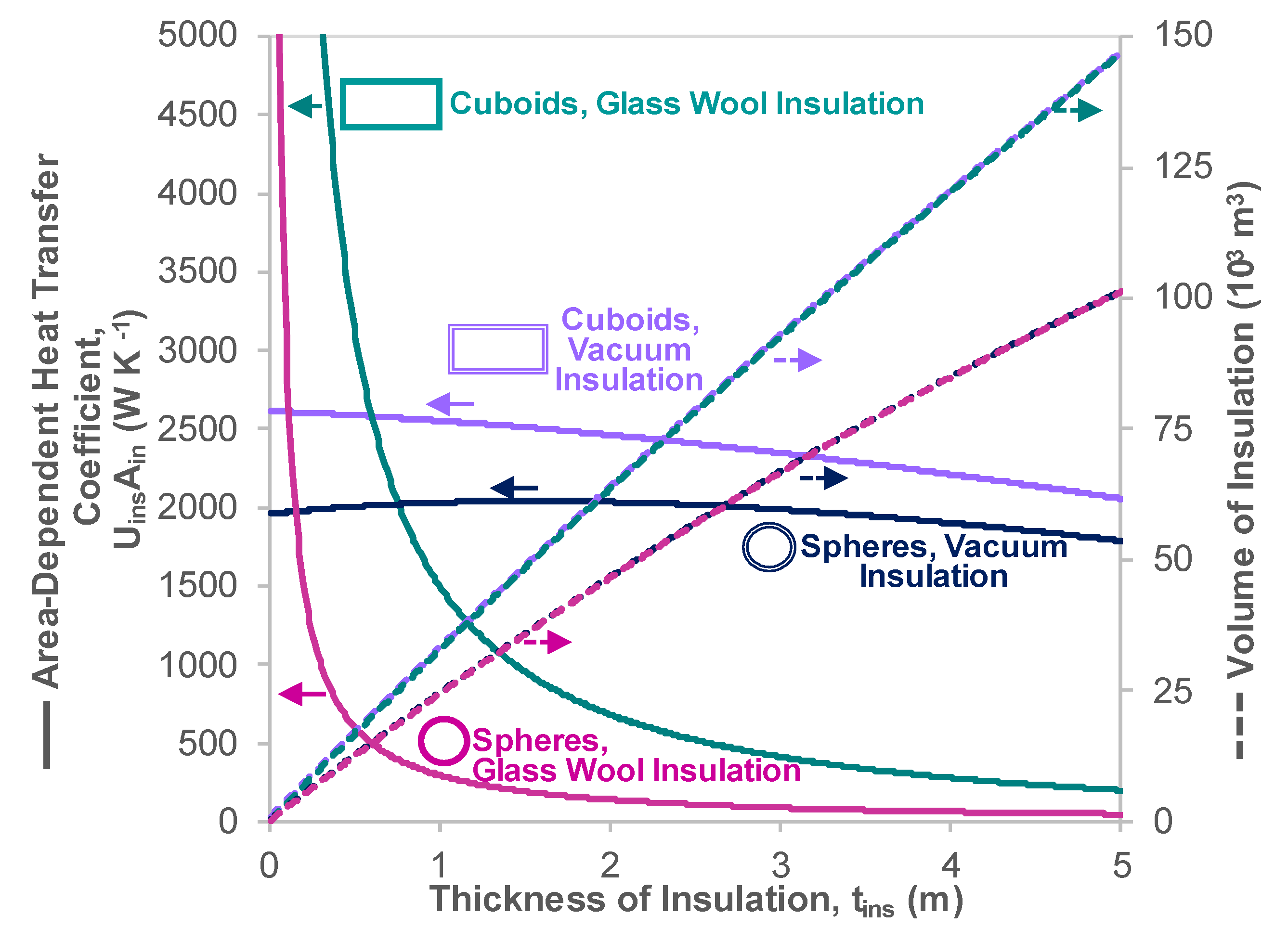
5.2. Effect of Insulation Thickness

The model is here used to compare the effect of varying the glass wool insulation thickness for the conventional LNG ship and the conceptual LH2 combustion ship without reliquefaction. Commonly, the insulation of an LNG ship is sized so that the BOR at the design point matches the fuel utilisation rate [7]. Figure 6 shows the variation of the BOR and fuel utilisation rate with the thickness of tank insulation for both ships. At each BN, the LNG ship velocities are selected so that the LNG ship’s BOR matches its fuel utilisation rate at an insulation thickness of 0.53 m (Figure 6a). In Figure 6b, the LH2 ship is assumed to have the same velocity as the LNG ship at each BN. However, the points at which the fuel utilisation rate matches the BOR occur at a higher insulation thickness than 0.53 m: they occur at thicknesses of 3.51 to 0.55 m for a BN of 0 to 12, respectively. Therefore, to insulate the LH2 ship to the same standards as the existing LNG ship, 1.04 to 6.62 times the insulation thickness is required, with more insulation being required at lower BN. It should be noted that, as hydrogen BOG has a negligible greenhouse effect relative to natural gas [11], it is likely that the insulation standards assumed here do not need to be met. However, the safety hazards of venting hydrogen BOG should not be disregarded. Relative to natural gas, hydrogen has similar risks associated with its physical and combustion properties [23].

5.3. Effect of Electrification

Here, the ability of all LNG, LH2 combustion, and LH2 electric ships to transport fuel at the design ship velocity and in calm weather (BN = 2) is investigated. The ship design variations are summarised in Table 10 and concisely represented using a key (comprising a specific colour and symbol). An optimised insulation thickness is selected for each tank design. As there are no fuel losses onboard ships with reliquefaction, a fair comparison of ship designs can be better achieved when maximising the mass of fuel remaining onboard the ship after 20 days. This voyage duration was chosen as it allowed the ship to reach typical voyage distances in the range of those recorded by El-Gohary [71] and Lasserre and Pelletier [72]. More specifically, at the design ship velocity, a 20 day-long voyage allows the ship to travel 14,890 km. The resulting component masses and volumes are detailed in Table 11, together with the fuel depletion and revenue loss rates. The latter value is determined by multiplying the fuel depletion rate (measured in ton/day) by current prices per ton of each fuel [73,74].
Note that the fuel depletion rates of the LH2 tanks without reliquefaction (~0.6%/day, see Table 11b) are of a similar order to the existing, stationary tank modelled in Al Ghafri et al. (~0.7 to 0.8%/day) [43]. This reinforces that the tanks are appropriately insulated for calm weather, despite not being insulated enough for the boil-off rate to be equal to the fuel utilization rate, as in Section 5.2. Should ships be designed to regularly travel in conditions rougher than BN = 2, a higher insulation thickness would be required to maximise the mass of fuel remaining onboard the ship, and higher fuel depletion rates would be expected.
Out of all the LH2 ship variants, the LH2 employing fuel cells has the highest spatial efficiency for fuel storage. Fuel cell ships deliver at least 1.1% more fuel than direct combustion ships. This is because the volume of engines is almost eliminated by electrifying them. The combined volume of fuel cells and electric engines is about 0.004% of the internal volume, whereas the internal combustion engines take up around 0.46% of the internal volume. The onboard space available for fuel is thus increased by 0.46% of the internal volume of the ship. Fuel cell ships also have a higher propulsion efficiency (Section 4.4), so the total fuel depletion rate of the LH2 fuel cell ship is 80.2% of that of the LH2 combustion ship.
Figure 7 shows the variation of remaining mass and energy of fuel with time for all investigated ships. The ships are operated at 16.7 kn and BN = 2. For all voyage lengths considered in this study, the LH2 electric ship that employs reliquefaction has the highest delivered mass of fuel out of all the LH2 ships due to its higher spatial efficiency and lower fuel depletion rate (see also Table 11). However, it should be noted that, relative to the existing LNG ship, it can only deliver 41.4% of the fuel energy for a voyage length of 5000 km, and 40.2% of the fuel energy for a voyage length of 15,000 km. It has revenue loss rates due to fuel depletion of 1.43 times those expected onboard the LNG ship (Table 11).
As discussed previously, ships that employ reliquefaction have a fuel depletion rate sensitive to the ship velocity and BN. If such variability must be avoided, the best-performing delivery fuel design is again the LH2 fuel cell ship. The resulting loss in delivered fuel is 9.1% at 5000 km and 13.4% at 15,000 km, which is equivalent to a revenue loss of $895,000 at 5000 km and $1,270,000 at 15,000 km [73,74].

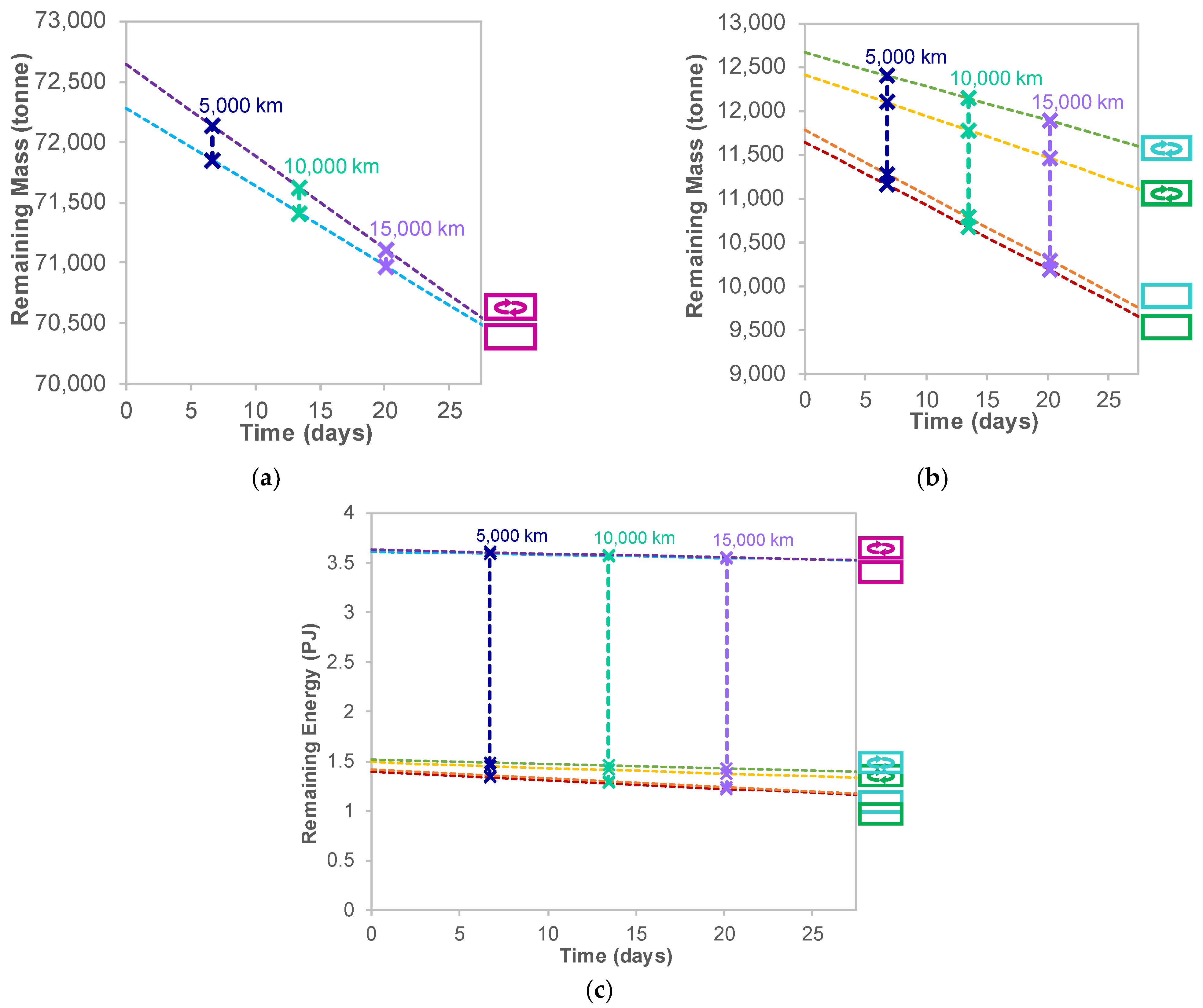
5.4. Additional Fuel Tank Design Variations

The model may also be used to investigate the BOR and fuel carrier properties of other conceptual LH2 ship designs than those presented previously. More detailed calculations were performed to understand vacuum insulation as an alternative to glass wool and the effects of fuel tank number and shape. The inputs and detailed results are given in Appendix B, Appendix C and Appendix D. It has been found that spherical tanks are more effective at eliminating sloshing effects than cuboidal tanks. The ship’s available volume is better utilised by cuboidal tanks only at low tank numbers. In terms of maximising the delivered fuel (but not minimising its variability), the best performing LH2 designs employ four vacuum insulated spherical tanks along with reliquefaction and electric propulsion. Such ship designs outperform all others due to their superior spatial efficiency and fuel depletion rate.

5.5. Sizing Considerations for Targeting a Specific Delivered Energy

To demonstrate how the present model can be used for further explorations into LH2 ship design and optimisation, sizing considerations for targeting specific delivered energy at the end of a voyage are made here. The total energy delivered by the conventional LNG carrier is set as the target, and the conceptual LH2 ship is re-sized accordingly. For the sake of simplicity, it is assumed that the volume of tank structure onboard the ship increases to hold the extra volume of fuel, whereas the BOR in %/day and the ballast water, engine, fuel cell, and unassigned volumes do not vary with the size of the ship.
To deliver the same energy as an LNG ship, the best performing LH2 ship in Section 5.3 (the LH2 ship with fuel cells and reliquefication) is required to carry approximately 2.42 times the volume of fuel for a voyage length of 5000 km and 2.49 times the volume of fuel for a voyage length of 15,000 km (see the delivered energies for this ship in Section 5.3). A ship carrying these fuel volumes requires approximately 18,300 m3 and 18,600 m3 of tank structure, respectively. The “Other Volumes” (Table 11) onboard the ship are assumed constant so that the resulting LH2 ships designed for 5000 km and 15,000 km voyages would be approximately 1.73 and 1.77 times the size of the LNG ship (based on internal volume). Such a ship would require major alterations to re-optimise design features such as its streamlining and stability, so its sizing and power consumption would differ significantly from those presented in this study.

6. Conclusions and Recommendations for Future Work

A model has been developed to estimate fuel boil-off rates (BOR) for cryogenic energy carrier vessels. The model is based on thermodynamic modelling of the fuel tank and empirically derived trends for required engine power, ship motion, and heat transfer enhancement due to sloshing at a range of ship velocities and weather conditions represented by Beaufort number (BN). BOR estimates are first calibrated using data for an existing liquefied natural gas (LNG) carrier, modelled as comprising four cryogenic fuel cuboidal tanks insulated by glass wool. Although not limited to any specific cryogenic fuel, the approach is then adapted for liquid hydrogen (LH2) as this fuel may have a crucial role in future decarbonised energy storage and transportation systems. Consequently, various candidate designs and configurations potentially suitable for future LH2 carriers are investigated. The analysis indicates that:
(1)
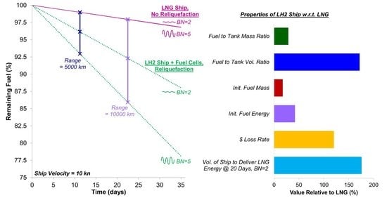
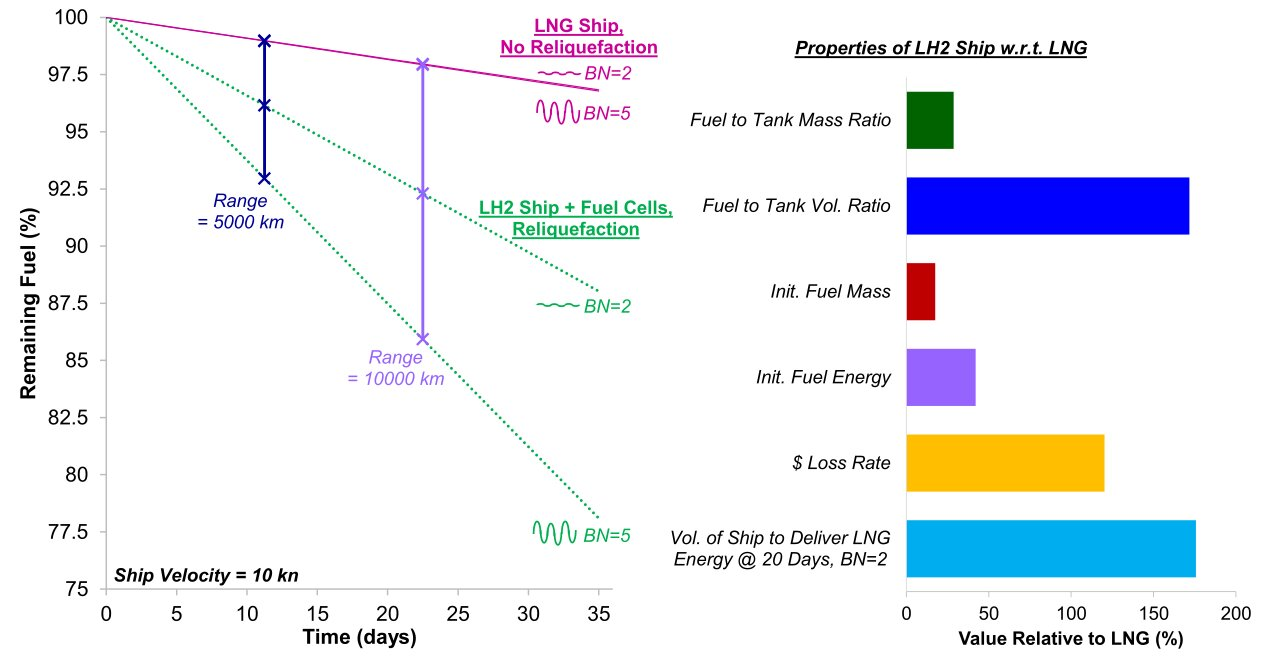
An LH2 carrier with the same fuel tank volume and insulation thickness as an LNG carrier can contain 16.8% of the fuel mass and 40.2% of the fuel energy. The unforced BOR of the LH2 carrier is 8.94 times higher than that of an LNG ship.
(2)
The heat transfer and boil-off effects of sloshing on an LH2 carrier are more significant than those on an LNG carrier. In particular, the rate of BOR increase with BN on board the LH2 ship is twice as large relative to an LNG carrier.
(3)
Adding a reliquefaction unit to the vessel reduces the fuel depletion rate by at least 38.7%. However, this reduction is highly dependent on the weather and ship velocity, so reliquefaction introduces a significantly higher sensitivity of the fuel depletion rate and delivered fuel to the operating conditions.
(4)
A parametric analysis illustrated that 1.04 to 6.62 times the insulation thickness of glass wool is required to allow the LH2 carrier to have BOR properties equivalent to the LNG ship, primarily due to the lower LH2 temperature.
(5)
An LH2 carrier powered by fuel cells and electric motors delivers at least 1.1% more cargo fuel than one with internal combustion engines due to the lower volume of the electric propulsion system and the higher efficiency of fuel cell and electric motor propulsion.
(6)
An LH2 carrier operating with fuel cells and reliquefaction must be at least 1.73 times larger by volume than the LNG carrier to deliver the same energy.
In summary, conceptual LH2 carriers require significant redesign if the BOR and fuel carrier standards of LNG carriers are to be achieved. This is also indicated by the effect of further alterations to the fuel tank, e.g., variations to the total number of tanks, their shape, and the insulation type.
The presented approach features a novel framework that relies on the integration of physical and empirical modelling to estimate the BOR properties of cryogenic fuel carriers from voyage conditions. The approach is extendable and amenable to updates as and when advances are made in the various sub-models relevant to ship motion, propulsion, sloshing, and heat transfer. The current formulation is suitable for comparing the properties of a wide variety of conceptual and existing cryogenic fuel carriers and is not limited to the variants of LH2 ship design detailed in this study. Future work should focus on validation against hydrodynamic and thermodynamic voyage data from real cryogenic ships and application to real-time prediction of BOR properties using onboard data acquisition.

Author Contributions

Conceptualization, J.R.S., S.G. and E.M.; methodology, J.R.S., S.G. and E.M.; software, J.R.S. and S.G.; validation, J.R.S., S.G. and E.M.; formal analysis, J.R.S.; data curation, J.R.S.; writing—original draft preparation, J.R.S.; writing—review and editing, J.R.S., S.G. and E.M.; visualization, J.R.S.; supervision, E.M.; funding acquisition, E.M. All authors have read and agreed to the published version of the manuscript.

Funding

Jessie Smith was funded by an EPSRC Doctoral Training Grant.

Data Availability Statement

The computational code leading to the results presented in this paper is available on request.

Acknowledgments

We thank Richard Gilmore from Maran Gas for his assistance with empirical data on tanks and boil-off rates.

Conflicts of Interest

The authors declare no conflict of interest.

Appendix A. Additional Data Tables

Table A1. Properties of sea water [67].
Value NameUnitQuantity
Density of Sea Waterkg m−31026
Dynamic ViscosityPa-s0.00117
Table A2. Power and fuel utilisation rates of the conventional LNG ship at velocities of 10 to 19.5 kn [28].
Velocity (kn)Propulsive Power (kW)Fuel Utilisation Rate (ton/day)
10344229
11453734
12583740
13733447
14903355
1510,93663
1613,03773
1715,34083
1817,87895
1920,746108
19.522,361115
Table A3. Inputs for sizing the reliquefaction unit and generator [75,76,77].
InputUnitQuantitySource
Volumetric Power Density of Heat Exchangers
in Reliquefaction Unit *
W m−375,700[75]
Estimated Percentage Volume of Aluminium
in Reliquefaction Unit Heat Exchangers *
%4[75]
Density of Aluminiumkg m−32700[76]
Gravimetric Power DensityW kg−11020[77]
Volumetric Power Density MW m−31.74[77]
* The reliquefaction unit is assumed to consist entirely of heat exchangers.

Appendix B. Variation of Boil-Off with Fuel Tank Number and Shape

Appendix B.1. Effect of Fuel Tank Number with Cuboidal Tanks

Sloshing can be reduced by dividing the fuel into a greater number of tanks, equivalent to using baffles, i.e., rigid boundaries within a tank that reduce fluid movement from one region of the tank to another [78]. This effect is here considered assuming that each tank onboard the cryogenic ship is evenly spaced along the ship’s length. For cuboidal tanks, each tank’s length is thus considered the length of the ship divided by the number of tanks onboard the ship. The same thickness of insulation is assumed to surround each tank, so that as the number of tanks increases an increased volume of tank material occupies the space onboard the ship available for cryogenic fuel. As the temperature between the tanks is assumed to be that of the external environment (Section 4.1), the surface area for heat ingress increases as the number of tanks increases.
Figure A1 shows the variation of total BOR onboard the LNG and LH2 ship with BN and tank number ( n ) at a velocity of 10 kn, utilising cuboidal tanks without a reliquefaction unit. It is evident that the effects of sloshing lead to a BOR increase with increasing BN and that sloshing effects decrease as the number of tanks increases (note the decreasing gradient of the curves). In contrast, the BOR increases with the number of tanks at any fixed BN since the tank surface area to volume ratio increases.
Figure A1. Variation of total boil-off rate with Beaufort number (BN) and number of fuel tanks ( n ) at a ship velocity ( v ship ) of 10 kn (a) An LNG ship; (b) An LH2 ship with the same insulation thickness as the LNG carrier, without reliquefaction.
Energies 15 02046 g0a1
As mentioned in Section 4.1, the conventional LNG ship contains four fuel tanks. At a tank number of n = 4 , the effects of sloshing onboard the LH2 ship are greater than those onboard the LNG ship, while the proportional increase in BOR from one to four tanks is lower. Therefore, an appropriate number of tanks onboard the LH2 ship is likely to be above four. This allows for a more significant reduction in sloshing effects while limiting the proportional increase in BOR to around that of the LNG ship. The increase in BOR with sloshing onboard an LH2 ship with eight tanks is of the same order as that of an LNG ship with four tanks. Nevertheless, the increase in BOR from one to eight tanks is 1.8 times that of an LNG ship when its tank number is increased from one to four tanks. Therefore, relative to the LNG ship, the increase in BOR that results from increasing the tank number yields a lower reduction in sloshing effects. This indicates that selecting the number of cuboidal tanks onboard the LH2 ship involves navigating a trade-off. The trade-off entails limiting the unforced BOR while also limiting its variation with ship operating conditions.

Appendix B.2. Conversion to Spherical Tanks

Like the cuboidal tanks, the spherical tanks must be sized so that the internal volume of the existing LNG ship is not exceeded. However, the tanks must also be sized to ensure that the tank radius cannot exceed half the ship’s beam. The number of tanks is important in this aspect. Concerning the insulation thickness of the conventional LNG ship investigated in this paper (Section 4.1), the spherical tank size is limited by the ship radius when n 4 , and by the internal volume when n > 4 . At an insulation thickness of 0.53 m, the total surface area for heat transfer of four spherical tanks is 24,300 m2, the total volume of tank material is 13,200 m3 and the U ins value is 0.023 W m−2 K−1 (based on the thermal conductivity of glass wool estimated in Section 4.1).
On the one hand, if the number of spherical tanks onboard the LH2 ship is increased up to four ( n 4 ), more tanks of the same size can be added to the ship; therefore, more fuel can be fitted onboard. This does not affect the surface area to volume ratio, so there is no increase in heat ingress from the external environment per unit volume of fuel. On the other hand, if n > 4 , the individual tank size decreases with increasing n (as with cuboidal tanks), increasing their surface area to volume ratio. Consequently, more insulation is added to the ship, decreasing the space available for fuel. At the same time, the BOR increases due to the additional heat transfer from the external to the internal environment.
The degree of sloshing in the spherical fuel tanks is less than in the cuboidal tanks. If the ship′s tilt is assumed to be small, the force distribution of the fuel weight around the ship’s centre of mass does not vary with tilting angle, so no unbalanced moment is produced by the tilt. Therefore, the amplitude of the fuel wave within the spherical tanks only depends on the force distributions that result from the hydrostatic and sea waves. In an LH2 ship with n = 4 , travelling at a velocity of 10 kn and BN = 5, the SSF above unity (SSF-1) is 67.5% of that of a ship carrying cuboidal tanks. It also follows that increasing the number of tanks has little effect on the decrease of SSF. For the same conditions, the SSF above unity only decreases by 20% when the tank number is increased from one to six tanks, whereas it decreases by 92% for a ship with cuboidal tanks.
In summary, as increasing the number of spherical tanks has little effect on sloshing, the number of spherical tanks should be selected to maximise the fuel stored on-board the ship while limiting the heat ingress from the external environment. An appropriate number of spherical tanks on board the ship modelled in this investigation is thus n = 4 .

Appendix C. Heat Transfer Properties of Vacuum Insulated Tanks

Vacuum casing insulation typically consists of a vacuum gap with a thin layer of structural material on each side. Here, it is assumed that aluminium is utilised for this purpose [79]. For a cuboidal tank with a vacuum gap thickness of 0.53 m at atmospheric pressure, 8 mm of aluminium is required at either side of the vacuum gap. For a spherical tank, 3.5 mm of aluminium is instead required (see Table A4 for the data used to calculate these values). It is assumed that heat transfer across the vacuum gap occurs predominantly due to radiation. Hence, the standard Stephan-Boltzmann equation for radiative heat transfer may be used to determine the heat transfer between two surfaces in an enclosure [80]. The insulation heat transfer coefficient, U ins , is 0.080 W m−2 K−1 when considering the emissivity of aluminium (see Table A4) and a vacuum gap thickness of 0.53 m for a cuboidal tank containing hydrogen. For a spherical tank, the value is 0.083 W m−2 K−1.
Table A4. Inputs for vacuum casing calculations [67,79,81].
InputUnitQuantitySource
Failure Stress of AluminiumMPa438[81]
Acceptable Ratio of Maximum Tensile Stress
to Failure Stress (mid-range value)
-1.7[79]
Emissivity of Aluminium-0.1[67]
The area-dependent heat transfer coefficient is the heat transfer coefficient of the insulation multiplied by the total surface area of external to internal heat transfer. Table A4 details its value, and the volume of insulation material, for four cuboidal and spherical tanks insulated by glass wool and vacuum casing at a thickness of 0.53 m. The insulation thickness for the vacuum casing is assumed to be the thickness of the vacuum gap. Similarly, the variation of area-dependent heat transfer coefficient and insulation volume with thickness is shown in Figure A2. Area-dependent heat transfer coefficients are shown for thicknesses from 1 cm to 5 m. For glass wool insulated tanks, the area-dependent heat transfer coefficient has an approximately inverse relationship to insulation thickness, while the tank volume is directly proportional to it. As unforced BOR is a function of heat ingress into the tank, the maximum delivered fuel mass occurs at a non-zero insulation thickness.
Table A5. Area-dependent heat transfer coefficient and volume of tank material for four tanks of insulation thickness of 0.53 m. Values for spherical and cuboidal tanks with glass wool and vacuum casing insulation are shown [67,79,81].
InputUnitTank ShapeInsulation TypeQuantitySource
Heat Transfer
Coefficient, U ins
W m−2 K−1CuboidGlass Wool0.092Section 4.1
CuboidVacuum Casing0.080This Section
SphereGlass Wool0.023Appendix B.2
SphereVacuum Casing0.083This Section
Surface Area for Heat Ingress Across Tank Wall, A in m2CuboidAny32,200Section 4.1
SphereAny24,300This Section
Area Dependent Heat Transfer
Coefficient U ins · A in
W K−1CuboidGlass Wool2960Above Rows
Vacuum Casing2590Above Rows
SphereGlass Wool570Above Rows
Vacuum Casing2010Above Rows
Volume of Tank Materialm3CuboidAny17,600Table 1
SphereAny13,200Appendix B.2
Figure A2. Variation of area-dependent heat transfer coefficient ( U ins · A in ) and volume with insulation thickness ( t ins ) for four spherical and cuboidal tanks insulated by glass wool and vacuum casing onboard an LH2 ship. Values are displayed for 0.01 to 5 m.
Energies 15 02046 g0a2
Conversely, the vacuum insulation’s area-dependent heat transfer coefficient does not change as rapidly with insulation thickness. As a result, the maximum delivered mass of fuel appears to occur at the minimum possible thickness of the vacuum gap. However, as only radiative heat transfer is considered in this analysis, the modelled vacuum heat transfer coefficient is somewhat idealised. In reality, structures such as pillars must span the vacuum gap to maintain their integrity. As a result, some heat loss via conduction across these structures leads to a high heat transfer coefficient, especially at low insulation thicknesses [82]. The maximum delivered mass of fuel thus occurs at a low but non-zero vacuum gap thickness. At high insulation thicknesses, glass wool is a superior insulator compared to vacuum casing. For example, at an insulation thickness of 3.51 m, the spherical vacuum insulated container has an area-dependent heat transfer coefficient of 26.15 times, and the cuboidal container 6.80 times, the insulation thickness of the equivalent glass wool containers. As the area-dependent heat transfer coefficient of vacuum insulation does not change significantly with insulation thickness, it is impossible to achieve the same standard of insulation achieved by glass wool at this thickness setting. However, below an insulation thickness of 0.61 m for cuboidal containers and 0.16 m for spherical containers, vacuum casing has a lower area-dependent heat transfer coefficient than glass wool, so vacuum casing can be considered a better insulator than glass wool when low insulation thicknesses are desired. It should be noted that, despite these favourable properties, vacuum insulation has both a higher cost and is heavier than glass wool at all insulation thicknesses [8].

Appendix D. Comparison of Additional Designs

As in Section 5.3, the model is employed to compare the ability of LNG, LH2 combustion, and LH2 electric ship designs to transport fuel at the design velocity and BN = 2. Here, the comparison includes the additional ship designs investigated in Appendix B and Appendix C. The ships are represented concisely using symbols identified by a key in Table A6, an extension of the key in Table 10. Again, the insulation thickness is optimised by maximising the mass of fuel remaining on board the ship after 20 days. As mentioned in Appendix C, it is impossible to insulate a ship that employs vacuum casing to the same standards as a glass wool ship, but vacuum casing is superior to glass wool insulation at low insulation thicknesses. Following the discussion in Appendix C, the vacuum gap is set to 0.01 m for all vacuum insulation ships. It is assumed that each ship has four fuel tanks. Table A7 provides an extension to Table 11, detailing the component masses, volumes, insulation thicknesses, fuel depletion rates, and revenue losses for all investigated designs.
Table A6. Key to identify the symbols that represent all investigated ship designs.
Ship VariableIdentifier TypeCategoriesIdentifierDemonstration
Fuel and
Propulsion Type
ColourMethane Internal Combustion EnginePink
Hydrogen Internal Combustion EngineGreen
Hydrogen ElectricLight Blue
Tank ShapeIcon ShapeCuboidRectangle Energies 15 02046 i001
SphereCircle Energies 15 02046 i002
Insulation TypeOutline TypeGlass WoolSingle Line Energies 15 02046 i003
Vacuum InsulationDouble Line Energies 15 02046 i004
Presence of ReliquefactionPresence of
Reliquefaction Symbol
Reliquefaction
Present
Symbol Present Energies 15 02046 i005
Reliquefaction
Absent
Symbol Absent
Out of all the LH2 ships, the LH2 fuel cell ship with vacuum insulated spherical tanks has the highest spatial efficiency for fuel storage. This is because, for spherical tanks, the same thickness of insulation takes up less volume relative to cuboidal tanks (see Appendix C). As a result, 36.1% of the ship’s total mass and 53% of its internal volume are occupied by fuel. Furthermore, Figure A3 shows the variation of remaining mass and energy of fuel with time for all the LH2 electric ships investigated. The ships are operated at the design point. For all voyage lengths considered in this study, the LH2 electric ship that employs vacuum insulated spherical tanks and reliquefaction has the highest delivered mass of fuel, again due to its high spatial efficiency and low fuel depletion rate. If variability in the mass of delivered fuel is undesirable, the best-performing delivery fuel design is the LH2 ship with vacuum insulated spherical tanks that does not use reliquefaction. The resulting loss in delivered fuel is 0.88% at 5000 km and 2.7% at 15,000 km, which is equivalent to a revenue loss of $93,000 at 5000 km and $279,000 at 15,000 km [73,74].
Table A7. Estimated ship properties, set to maximise the delivered mass after 20 days for all investigated ship designs: (a) thickness of insulation and component masses; (b) component volumes, fuel depletion rate, and revenue loss rate [73,74].
(a)
Fuel and
Propulsion Type
Ship TypeThickness of
Insulation (m)
Initial Mass of Fuel (103 ton)Mass of Tank (103 ton)Other Masses (103 ton)
Methane
Internal
Combustion
Engine
Energies 15 02046 i0060.5372.290.8523.62
Energies 15 02046 i0070.0171.671.4623.62
Energies 15 02046 i0080.0773.050.0923.62
Energies 15 02046 i0090.0172.600.5323.62
Energies 15 02046 i0100.3172.640.4923.62
Energies 15 02046 i0110.0171.671.4623.62
Energies 15 02046 i0120.0773.050.0923.62
Energies 15 02046 i0130.0172.600.5323.62
Hydrogen
Internal
Combustion
Engine
Energies 15 02046 i0140.7211.651.1423.87
Energies 15 02046 i0150.0113.241.6023.87
Energies 15 02046 i0160.2612.850.3123.87
Energies 15 02046 i0170.0113.270.5323.87
Energies 15 02046 i0180.3812.420.6123.87
Energies 15 02046 i0190.0113.241.6023.87
Energies 15 02046 i0200.1713.000.2123.87
Energies 15 02046 i0210.0113.270.5323.87
Hydrogen Fuel Cell Energies 15 02046 i0220.7111.781.1323.18
Energies 15 02046 i0230.0113.351.6223.18
Energies 15 02046 i0240.2612.960.3223.18
Energies 15 02046 i0250.0113.390.5423.18
Energies 15 02046 i0260.3212.670.5223.18
Energies 15 02046 i0270.0113.351.6223.18
Energies 15 02046 i0280.1513.150.1823.18
Energies 15 02046 i0290.0113.390.5423.18
(b)
Fuel and
Propulsion Type
Ship TypeVolume of Tank
(103 m3)
Other
Volumes
(103 m3)
Fuel
Depletion Rate
(%/day)
Revenue Loss Rate
(103 $/day)
Methane
Internal
Combustion
Engine
Energies 15 02046 i03017.62171.970.090521.6
Energies 15 02046 i0310.84190.240.104324.7
Energies 15 02046 i0321.78171.970.089521.6
Energies 15 02046 i0330.44171.970.090121.6
Energies 15 02046 i03410.20178.540.104825.1
Energies 15 02046 i0350.84190.240.094422.3
Energies 15 02046 i0361.78171.970.089521.6
Energies 15 02046 i0370.44171.970.090121.6
Hydrogen
Internal
Combustion
Engine
Energies 15 02046 i03823.79171.970.622457.7
Energies 15 02046 i0390.90171.970.594562.6
Energies 15 02046 i0406.55171.970.168117.2
Energies 15 02046 i0410.44171.970.268628.4
Energies 15 02046 i04212.70171.970.381637.7
Energies 15 02046 i0430.90171.970.246325.9
Energies 15 02046 i0444.30171.970.170217.6
Energies 15 02046 i0450.44171.970.175818.6
Hydrogen Fuel Cell Energies 15 02046 i04623.57170.310.625858.6
Energies 15 02046 i0470.91170.310.590762.8
Energies 15 02046 i0486.59170.310.167617.3
Energies 15 02046 i0490.44170.310.267828.5
Energies 15 02046 i05010.76170.310.306130.9
Energies 15 02046 i0510.91170.310.180019.1
Energies 15 02046 i0523.82170.310.144015.1
Energies 15 02046 i0530.44170.310.137714.7
Figure A3. Variation of remaining fuel mass and energy with voyage duration at BN = 2 and a resultant velocity of 16.7 knots. All investigated LH2 fuel cell ships are shown at the insulation thickness that maximises the fuel delivered after a voyage of 20 days.
Energies 15 02046 g0a3

References

  1. Raj, R.; Ghandehariun, S.; Kumar, A.; Geng, J.; Linwei, M. A techno-economic study of shipping LNG to the Asia-Pacific from Western Canada by LNG carrier. J. Nat. Gas Sci. Eng. 2016, 34, 979–992. [Google Scholar] [CrossRef]
  2. The Hydrogen Council Hydrogen Decarbonization Pathways. Available online: https://hydrogencouncil.com/wp-content/uploads/2021/01/Hydrogen-Council-Report_Decarbonization-Pathways_Executive-Summary.pdf (accessed on 6 February 2022).
  3. Fernández, I.A.; Gómez, M.R.; Gómez, J.R.; López-González, L.M. H2 production by the steam reforming of excess boil off gas on LNG vessels. Energy Convers. Manag. 2017, 134, 301–313. [Google Scholar] [CrossRef]
  4. Krikkis, R.N. A thermodynamic and heat transfer model for LNG ageing during ship transportation. Towards an efficient boil-off gas management. Cryogenics 2018, 92, 76–83. [Google Scholar] [CrossRef]
  5. Ekanem Attah, E.; Bucknall, R. An analysis of the energy efficiency of LNG ships powering options using the EEDI. Ocean Eng. 2015, 110, 62–74. [Google Scholar] [CrossRef]
  6. Qu, Y.; Noba, I.; Xu, X.; Privat, R.; Jaubert, J.N. A thermal and thermodynamic code for the computation of Boil-Off Gas–Industrial applications of LNG carrier. Cryogenics 2019, 99, 105–113. [Google Scholar] [CrossRef]
  7. Schönsteiner, K.; Massier, T.; Hamacher, T. Sustainable transport by use of alternative marine and aviation fuels—A well-to-tank analysis to assess interactions with Singapore’s energy system. Renew. Sustain. Energy Rev. 2016, 65, 853–871. [Google Scholar] [CrossRef]
  8. Banaszkiewicz, T.; Chorowski, M.; Gizicki, W.; Jedrusyna, A.; Kielar, J.; Malecha, Z.; Piotrowska, A.; Polinski, J.; Rogala, Z.; Sierpowski, K.; et al. Liquefied Natural Gas in Mobile Applications—Opportunities and Challenges. Energies 2020, 13, 5673. [Google Scholar] [CrossRef]
  9. McFarlan, A. Techno-economic assessment of pathways for liquefied natural gas (LNG) to replace diesel in Canadian remote northern communities. Sustain. Energy Technol. Assess. 2020, 42, 100821. [Google Scholar] [CrossRef]
  10. Awoyomi, A.; Patchigolla, K.; Anthony, E.J. Process and Economic Evaluation of an Onboard Capture System for LNG-Fueled CO2 Carriers. Ind. Eng. Chem. Res. 2020, 59, 6951–6960. [Google Scholar] [CrossRef]
  11. IPCC. Climate Change 2007: The Physical Science Basis. In Contribution of Working Group I to the Fourth Assessment Report of the Intergovernmental Panel on Climate Change; Solomon, S., Qin, D., Manning, M., Chen, Z., Marquis, M., Averyt, K.B., Tignor, M., Miller, H.L., Eds.; Cambridge University Press: Cambridge, UK; New York, NY, USA, 2007; Volume 59, p. 996. [Google Scholar]
  12. Wijayanta, A.T.; Oda, T.; Purnomo, C.W.; Kashiwagi, T.; Aziz, M. Liquid hydrogen, methylcyclohexane, and ammonia as potential hydrogen storage: Comparison review. Int. J. Hydrog. Energy 2019, 44, 15026–15044. [Google Scholar] [CrossRef]
  13. Hansson, J.; Månsson, S.; Brynolf, S.; Grahn, M. Alternative marine fuels: Prospects based on multi-criteria decision analysis involving Swedish stakeholders. Biomass Bioenergy 2019, 126, 159–173. [Google Scholar] [CrossRef]
  14. Al-Breiki, M.; Bicer, Y. Investigating the technical feasibility of various energy carriers for alternative and sustainable overseas energy transport scenarios. Energy Convers. Manag. 2020, 209, 112652. [Google Scholar] [CrossRef]
  15. Güler, E.; Ergin, S. An investigation on the solvent based carbon capture and storage system by process modeling and comparisons with another carbon control methods for different ships. Int. J. Greenh. Gas Control 2021, 110, 103438. [Google Scholar] [CrossRef]
  16. A Seamless Hydrogen Supply Chain. Available online: https://media.nature.com/original/magazine-assets/d42473-020-00544-8/d42473-020-00544-8.pdf (accessed on 6 February 2022).
  17. Kawasaki Develops Cargo Containment System for Large Liquefied Hydrogen Carrier with World’s Highest Carrying Capacity—AiP Obtained from ClassNK. Available online: https://global.kawasaki.com/en/corp/newsroom/news/detail/?f=20210506_9983 (accessed on 6 February 2022).
  18. Kamiya, S.; Nishimura, M.; Harada, E. Study on introduction of CO2 free energy to Japan with liquid hydrogen. Phys. Procedia 2015, 67, 11–19. [Google Scholar] [CrossRef] [Green Version]
  19. Ahn, J.; You, H.; Ryu, J.; Chang, D. Strategy for selecting an optimal propulsion system of a liquefied hydrogen tanker. Int. J. Hydrog. Energy 2017, 42, 5366–5380. [Google Scholar] [CrossRef]
  20. Alkhaledi, A.N.F.N.R.; Sampath, S.; Pilidis, P. A hydrogen fuelled LH2 tanker ship design. Ships Offshore Struct. 2021, 1–10. [Google Scholar] [CrossRef]
  21. Korberg, A.D.; Brynolf, S.; Grahn, M.; Skov, I.R. Techno-economic assessment of advanced fuels and propulsion systems in future fossil-free ships. Renew. Sustain. Energy Rev. 2021, 142, 110861. [Google Scholar] [CrossRef]
  22. Leo, T.J.; Durango, J.A.; Navarro, E. Exergy analysis of PEM fuel cells for marine applications. Energy 2010, 35, 1164–1171. [Google Scholar] [CrossRef]
  23. Klebanoff, L.E.; Pratt, J.W.; LaFleur, C.B. Comparison of the safety-related physical and combustion properties of liquid hydrogen and liquid natural gas in the context of the SF-BREEZE high-speed fuel-cell ferry. Int. J. Hydrog. Energy 2017, 42, 757–774. [Google Scholar] [CrossRef] [Green Version]
  24. Marandi, S.; Mohammadkhani, F.; Yari, M. An efficient auxiliary power generation system for exploiting hydrogen boil-off gas (BOG) cold exergy based on PEM fuel cell and two-stage ORC: Thermodynamic and exergoeconomic viewpoints. Energy Convers. Manag. 2019, 195, 502–518. [Google Scholar] [CrossRef]
  25. Liu, Z.; Li, C. Influence of slosh baffles on thermodynamic performance in liquid hydrogen tank. J. Hazard. Mater. 2018, 346, 253–262. [Google Scholar] [CrossRef] [PubMed]
  26. Lee, D.H.; Cha, S.J.; Kim, J.D.; Kim, J.H.; Kim, S.K.; Lee, J.M. Practical prediction of the boil-off rate of independent-type storage tanks. J. Mar. Sci. Eng. 2021, 9, 36. [Google Scholar] [CrossRef]
  27. Hydrogen as Marine Fuel. Available online: https://absinfo.eagle.org/acton/attachment/16130/f-bd25832f-8a70-4cc9-b75f-3aadf5d5f259/1/-/-/-/-/hydrogen-as-marine-fuel-whitepaper-21111.pdf (accessed on 6 February 2022).
  28. Available online: https://www.tradewindsnews.com/gas/maran-gas-maritime-extends-lng-orderbook-with-dsme-option-duo/2-1-1164038 (accessed on 6 February 2022).
  29. Petitpas, G. Boil-Off Losses along LH2 Pathway; LLNL-TR-750685936219; U.S. Department of Energy: Washington, DC, USA, 2018. [CrossRef]
  30. Maekawa, K.; Takeda, M.; Hamaura, T.; Suzuki, K.; Miyake, Y.; Matsuno, Y.; Fujikawa, S.; Kumakura, H. First experiment on liquid hydrogen transportation by ship inside Osaka bay. IOP Conf. Ser. Mater. Sci. Eng. 2017, 278, 012066. [Google Scholar] [CrossRef]
  31. Maekawa, K.; Takeda, M.; Miyake, Y.; Kumakura, H. Sloshing measurements inside a liquid hydrogen tank with external-heating-type MGB2 level sensors during marine transportation by the training ship Fukae-Maru. Sensors 2018, 18, 3694. [Google Scholar] [CrossRef] [PubMed] [Green Version]
  32. Wei, G.; Zhang, J. Numerical study of the filling process of a liquid hydrogen storage tank under different sloshing conditions. Processes 2020, 8, 1020. [Google Scholar] [CrossRef]
  33. Behruzi, P.; Gaulke, D.; Haake, D.; Brosset, L. Modeling of impact waves in LNG ship tanks. Int. J. Offshore Polar Eng. 2017, 27, 18–26. [Google Scholar] [CrossRef]
  34. Grotle, E.L.; Aesoy, V. Numerical simulations of sloshing and the thermodynamic response due to mixing. Energies 2017, 10, 1338. [Google Scholar] [CrossRef] [Green Version]
  35. Wu, S.; Ju, Y. Numerical study of the boil-off gas (BOG) generation characteristics in a type C independent liquefied natural gas (LNG) tank under sloshing excitation. Energy 2021, 223, 120001. [Google Scholar] [CrossRef]
  36. Yu, P.; Yin, Y.-C.; Wei, Z.-J.; Yue, Q.-J. A prototype test of dynamic boil-off gas in liquefied natural gas tank containers. Appl. Therm. Eng. 2020, 180, 115817. [Google Scholar] [CrossRef]
  37. Mir, H.; Ratlamwala, T.A.H.; Hussain, G.; Alkahtani, M.; Abidi, M.H. Impact of sloshing on fossil fuel loss during transport. Energies 2020, 13, 2625. [Google Scholar] [CrossRef]
  38. Ludwig, C.; Dreyer, M.E.; Hopfinger, E.J. Pressure variations in a cryogenic liquid storage tank subjected to periodic excitations. Int. J. Heat Mass Transf. 2013, 66, 223–234. [Google Scholar] [CrossRef]
  39. Igbadumhe, J.F.; Fürth, M. Hydrodynamic analysis techniques for coupled seakeeping-sloshing in zero speed vessels: A review. J. Offshore Mech. Arct. Eng. 2020, 143, 1–37. [Google Scholar] [CrossRef]
  40. Faltinsen, O.M. Hydrodynamics of marine and offshore structures. J. Hydrodyn. 2015, 26, 835–847. [Google Scholar] [CrossRef]
  41. Jeong, S.; Jeong, D.; Park, J.; Kim, S.; Kim, B. A voyage optimization model of LNG carriers considering boil-off gas. In Proceedings of the OCEANS 2019 MTS/IEEE SEATTLE, Seattle, WA, USA, 27–31 October 2019. [Google Scholar] [CrossRef]
  42. Mitra, S.; Wang, C.Z.; Reddy, J.N.; Khoo, B.C. A 3D fully coupled analysis of nonlinear sloshing and ship motion. Ocean Eng. 2012, 39, 1–13. [Google Scholar] [CrossRef]
  43. Al Ghafri, S.Z.S.; Swanger, A.; Jusko, V.; Siahvashi, A.; Perez, F.; Johns, M.L.; May, E.F. Modelling of Liquid Hydrogen Boil-Off. Energies 2022, 15, 1149. [Google Scholar] [CrossRef]
  44. Goodwin, D.G.; Speth, R.L.; Moffat, H.K.; Weber, B.W. Cantera: An Object-Oriented Software Toolkit for Chemical Kinetics, Thermodynamics, and Transport Processes; European Organization for Nuclear Research: Genève, Switzerland, 2021. [Google Scholar] [CrossRef]
  45. Kim, S.; Hwang, H.; Kim, Y.; Park, S.; Nam, K.; Park, J.; Lee, I. Operational Optimization of Onboard Reliquefaction System for Liquefied Natural Gas Carriers. Ind. Eng. Chem. Res. 2020, 59, 10976–10986. [Google Scholar] [CrossRef]
  46. Son, H.; Kim, J. Automated process design and integration of precooling for energy-efficient BOG (boil-off gas) liquefaction processes. Appl. Therm. Eng. 2020, 181, 116014. [Google Scholar] [CrossRef]
  47. Son, H.; Kim, J. Energy-efficient process design and optimization of dual-expansion systems for BOG (Boil-off gas) Re-liquefaction process in LNG-fueled ship. Energy 2020, 203, 117823. [Google Scholar] [CrossRef]
  48. Wang, Z.; Han, F.; Ji, Y.; Li, W. Case Studies in Thermal Engineering Analysis on feasibility of a novel cryogenic heat exchange network with liquid nitrogen regeneration process for onboard liquefied natural gas reliquefaction. Case Stud. Therm. Eng. 2020, 22, 100760. [Google Scholar] [CrossRef]
  49. Molland, A.; Turnock, S.; Hudson, D. Ship Resistance and Propulsion: Practical Estimation of Propulsive Power; Cambridge University Press: Cambridge, UK, 2011; ISBN 0521760526; 9780521760522. [Google Scholar]
  50. Chi, Y.; Fuxin, H.; Francis, N. Practical evaluation of the drag of a ship for design and optimization. J. Hydrodyn. 2013, 25, 645–654. [Google Scholar] [CrossRef]
  51. Moser, C.S.; Wier, T.P.; Grant, J.F.; First, M.R.; Tamburri, M.N.; Ruiz, G.M.; Miller, A.W.; Drake, L.A. Quantifying the total wetted surface area of the world fleet: A first step in determining the potential extent of ships’ biofouling. Biol. Invasions 2016, 18, 265–277. [Google Scholar] [CrossRef]
  52. Solomon, D.G.; Greco, A.; Masselli, C.; Gundabattini, E.; Rassiah, R.S. A Review on Methods to Reduce Weight and to Increase Efficiency of Electric Motors Using Lightweight Materials, Novel Manufacturing Processes, Magnetic Materials and Cooling Methods. Ann. Chim.-Sci. Des Matériaux 2020, 44, 1–14. [Google Scholar] [CrossRef]
  53. Aliasand, A.E.; Josh, F.T. Selection of Motor foran Electric Vehicle: A Review. Mater. Today Proc. 2020, 24, 1804–1815. [Google Scholar] [CrossRef]
  54. Wang, G.; Yu, Y.; Liu, H.; Gong, C.; Wen, S.; Wang, X.; Tu, Z. Progress on design and development of polymer electrolyte membrane fuel cell systems for vehicle applications: A review. Fuel Process. Technol. 2018, 179, 203–228. [Google Scholar] [CrossRef]
  55. Chen, Q.; Zhang, G.; Zhang, X.; Sun, C.; Jiao, K.; Wang, Y. Thermal management of polymer electrolyte membrane fuel cells: A review of cooling methods, material properties, and durability. Appl. Energy 2021, 286, 116496. [Google Scholar] [CrossRef]
  56. Kifune, H.; Zadhe, M. Efficiency Estimation of Synchronous Generators for Marine Applications and Verification with Shop Trial Data and Real Ship Operation Data. IEEE Trans. J. 2020, 8, 195541–195550. [Google Scholar] [CrossRef]
  57. Lee, H.; Shao, Y.; Lee, S.; Roh, G.; Chun, K.; Kang, H. Analysis and assessment of partial re-liquefaction system for liquefied hydrogen tankers using liquefied natural gas (LNG)and H2 hybrid propulsion. Int. J. Hydrog. Energy 2019, 44, 15056–15071. [Google Scholar] [CrossRef]
  58. Beaufort Scale. Available online: https://www.britannica.com/science/Beaufort-scale (accessed on 6 February 2022).
  59. Xue, H.; Chai, T. Path Optimization along Buoys Based on the Shortest Path Tree with Uncertain Atmospheric and Oceanographic Data. Comput. Intell. Neurosci. 2021, 2021, 1–7. [Google Scholar] [CrossRef]
  60. Le Gouriérès, D. Chapter I-The Wind. In Wind Power Plants; Le Gouriérès, D.B.T.-W.P.P., Ed.; Pergamon: Oxford, UK, 1982; pp. 1–29. ISBN 978-0-08-029966-2. [Google Scholar]
  61. Lin, C.S.; Van Dresar, N.T.; Hasan, M.M. Pressure control analysis of cryogenic storage systems. J. Propuls. Power 2004, 20, 480–485. [Google Scholar] [CrossRef] [Green Version]
  62. Tonnage Shipping. Available online: https://www.britannica.com/technology/gross-tonnage (accessed on 6 February 2022).
  63. Maran Gas Amphipolis. Available online: https://www.vesselfinder.com/vessels/MARAN-GAS-AMPHIPOLIS-IMO-9701217-MMSI-241414000 (accessed on 6 February 2022).
  64. Acoustic and Thermal Insulating Materials. In Building Decorative Materials; Li, Y.; Ren, S.; Zhou, Y.; Liu, H. (Eds.) Woodhead Publishing: Cambridge, UK, 2011; pp. 359–374. [Google Scholar] [CrossRef]
  65. MAN Diesel & Turbo Marine Engine Programme. Available online: https://www.man-es.com/docs/default-source/marine/marine-engine-programme-20205656db69fafa42b991f030191bb3bbb4.pdf?sfvrsn=9cac9964_42 (accessed on 6 February 2022).
  66. World of Change: Global Temperatures-NASA. Available online: https://earthobservatory.nasa.gov/world-of-change/decadaltemp.php (accessed on 6 February 2022).
  67. Perry, R.H.; Green, D.W.; Maloney, J.O. Perry’s Chemical Engineers’ Handbook; McGraw-Hill: New York, NY, USA, 1984; ISBN 0070494797. [Google Scholar]
  68. Klell, M. Storage of Hydrogen in the Pure Form. In Handbook of Hydrogen Storage: New Materials for Future Energy Storage; John Wiley & Sons, Inc.: Hoboken, NJ, USA, 2010; pp. 1–37. [Google Scholar] [CrossRef]
  69. Bong, U.; Im, C.; Yoon, J.; An, S.; Jung, S. Investigation on Key Parameters of NI HTS Field Coils for High Power Density Synchronous Motors. IEEE Trans. Appl. Supercond. 2021, 31, 1–5. [Google Scholar] [CrossRef]
  70. Wang, Y.; Ruiz Diaz, D.F.; Chen, K.S.; Wang, Z.; Adroher, X.C. Materials, technological status, and fundamentals of PEM fuel cells—A review. Mater. Today 2019, 32, 178–203. [Google Scholar] [CrossRef]
  71. El-Gohary, M.M. The future of natural gas as a fuel in marine gas turbine for LNG carriers. Proc. Inst. Mech. Eng. Part M J. Eng. Marit. Environ. 2012, 226, 371–377. [Google Scholar] [CrossRef]
  72. Lasserre, F.; Pelletier, S. Polar super seaways? Maritime transport in the Arctic: An analysis of shipowners’ intentions. J. Transp. Geogr. 2011, 19, 1465–1473. [Google Scholar] [CrossRef]
  73. Natural Gas Prices in 2021. Available online: https://www.switch-plan.co.uk/compare-energy-prices/gas/natural-gas/ (accessed on 6 February 2022).
  74. Brown, T. The Cost of Hydrogen: Platts Launches Hydrogen Price Assessment. Available online: https://www.ammoniaenergy.org/articles/the-cost-of-hydrogen-platts-launches-hydrogen-price-assessment/ (accessed on 6 February 2022).
  75. Chang, H.M.; Chung, M.J.; Kim, M.J.; Park, S.B. Thermodynamic design of methane liquefaction system based on reversed-Brayton cycle. Cryogenics 2009, 49, 226–234. [Google Scholar] [CrossRef]
  76. Chauhan, K.P.S. Influence of Heat Treatment on the Mechanical Properties of Aluminium Alloys (6xxx Series): A Literature Review. Int. J. Eng. Res. 2017, V6, 386–389. [Google Scholar] [CrossRef]
  77. Ghassemi, M. High power density technologies for large generators and motors for marine applications with focus on electrical insulation challenges. High Volt. 2020, 5, 7–14. [Google Scholar] [CrossRef]
  78. Xue, M.A.; Jiang, Z.; Hu, Y.A.; Yuan, X. Numerical study of porous material layer effects on mitigating sloshing in a membrane LNG tank. Ocean Eng. 2020, 218, 108240. [Google Scholar] [CrossRef]
  79. Mital, S.K.; Gyekenyesi, J.Z.; Arnold, S.M.; Sullivan, R.M.; Manderscheid, J.M.; Murthy, P.L.N. Review of Current State of the Art and Key Design Issues with Potential Solutions for Liquid Hydrogen Cryogenic Storage Tank Structures for Aircraft Applications. Available online: https://ntrs.nasa.gov/archive/nasa/casi.ntrs.nasa.gov/20060056194.pdf (accessed on 6 February 2022).
  80. Siegel, R.; Howell, J.R. Thermal Radiation Heat Transfer; McGraw-Hill: New York, NY, USA, 1971; Volume III. [Google Scholar]
  81. Chen, Y.; Clausen, A.H.; Hopperstad, O.S.; Langseth, M. Stress-strain behaviour of aluminium alloys at a wide range of strain rates. Int. J. Solids Struct. 2009, 46, 3825–3835. [Google Scholar] [CrossRef] [Green Version]
  82. Kim, J.; Jang, C.; Song, T.H. Combined heat transfer in multi-layered radiation shields for vacuum insulation panels: Theoretical/numerical analyses and experiment. Appl. Energy 2012, 94, 295–302. [Google Scholar] [CrossRef]
Figure 1. Control volume for liquid and vapour phases of cryogenic fuel in an unsealed container and control surface for the liquid-vapour interface. The cryogenic tank is assumed to operate without reliquefaction. Thermodynamic properties are shown, including the temperature of liquid ( T L ), vapour ( T V ), and external environment ( T out ); the mass of liquid ( M L ) and vapour ( M V ); the heat transfer rate into the liquid ( Q ˙ L ), into the vapour ( Q ˙ V ) and across the liquid-vapour interface ( Q ˙ if ); the rate of change of the internal energy of the liquid ( U ˙ L ) and vapour ( U ˙ V ); the specific enthalpy flow out of the liquid ( h L ) and through the vapour ( h V ); the mass flow rate out of the liquid ( m ˙ L ) and vapour ( m ˙ V ) the kinetic energy transfer rate due to sloshing ( W ˙ slosh ).
Energies 15 02046 g001
Figure 2. Control volume for liquid and vapour phases of cryogenic fuel in an unsealed container, and control surface for the liquid-vapour interface. The cryogenic tank is assumed to operate with reliquefaction. Thermodynamic properties are shown, which include: the temperature of liquid ( T L ), vapour ( T V ) and external environment ( T out ); the mass of liquid ( M L ) and vapour ( M V ); the heat transfer rate into the liquid ( Q ˙ L ), into the vapour ( Q ˙ V ) and across the liquid-vapour interface ( Q ˙ if ); the rate of change of the internal energy of the liquid ( U ˙ L ) and vapour ( U ˙ V ); the specific enthalpy flow out of the liquid ( h L ) and through the vapour ( h V ); the mass flow rate out of the liquid ( m ˙ L ) and vapour ( m ˙ V ); the rate of fuel reliquefaction ( m ˙ reliq ); the kinetic energy transfer rate due to sloshing ( W ˙ slosh ); and enthalpy extraction rate during the reliquefaction process ( W ˙ reliq ).
Energies 15 02046 g002
Figure 3. Force distributions acting upon a tilting ship carrying liquid fuel.
Energies 15 02046 g003
Figure 4. Sea and fuel properties involved in the calculation of heat transfer enhancement due to sloshing as a function of Beaufort number (BN). The trends shown are: (a) Velocity of the wind ( v wind ), sea ( v sea ), and liquefied natural gas ship at rated power ( v ship ); (b) Frequency of sea ( ω sea ) and liquefied natural gas waves at rated power ( ω L ); (c) Amplitude of sea ( D sea ) and liquefied natural gas waves at rated power ( D L ); (d) Sloshing scaling factor (SSF) of liquefied natural gas at a ship velocity of 0 kn and at rated power.
Energies 15 02046 g004
Figure 5. Variation of key mass flow rates with Beaufort number (BN) and ship velocity ( v ship ). The trends shown are: (a) fuel utilisation rate for propulsion ( m ˙ use ) and BOR ( m ˙ loss + m ˙ use ) for an existing LNG ship model; (b) fuel utilisation rate for propulsion ( m ˙ use ) and BOR ( m ˙ loss + m ˙ use ) for an LH2 combustion ship with the same tank insulation thickness as the LNG ship, without reliquefaction; (c) fuel utilisation rates for propulsion ( m ˙ use ) and reliquefaction ( m ˙ r - use ) for an LH2 combustion ship with the same tank insulation thickness as the LNG ship, with reliquefaction.
Energies 15 02046 g005
Figure 6. Variation of boil-off ( m ˙ use + m ˙ loss ) and fuel utilisation rate ( m ˙ use ) with insulation thickness, at Beaufort numbers (BN) of 0 to 12 and ship velocities ( v ship ) of 16.9, 16.9, 16.7, 16.4, 15.2, 11.8, 7.06, 3.50, 1.63, 0.779, 0.390, 0.205 and 0.113 knots, respectively. The ship models are: (a) an LNG ship; and (b) an LH2 combustion ship without reliquefaction.
Energies 15 02046 g006
Figure 7. Variation of remaining fuel mass and energy with voyage duration at BN = 2 and a ship velocity of 16.7 knots. All investigated ships are shown at the insulation thickness that maximises the fuel delivered after a voyage of 20 days. The trends shown are (a) the remaining mass onboard all LNG ships; (b) the remaining mass onboard all LH2 ships; (c) the remaining energy onboard all investigated ships.
Energies 15 02046 g007
Table 1. Data for the conventional LNG ship [28,63,64].
InputUnitQuantitySource
Number of Tanks-4[28]
Deadweightton95,190[63]
Density of Glass Woolkg m−348[64]
Fraction of Fuel Vapour%2[28]
Fuel Capacitym3173,600[28]
Gross Tonnageton113,000[63]
Rated PowerMW23.4[28]
Ship Beamm46[63]
Ship Lengthm295[63]
Thickness of Glass Woolm0.53[28]
Reliquefaction Unit PresentTrue/FalseFalse[28]
Table 2. MAN B&W 6G70ME-C engine data [65].
InputUnitQuantity
Rated PowerMW21.84
Masston665
Estimated Volume m31568
Table 5. LNG and LH2 properties at the design point [14,28,44,67,68].
InputUnitQuantity
Natural GasSourceHydrogenSource
Temperature of LiquidK110[28]20.15[14]
Density of Liquidkg m−3425[28]70.95[44]
Temperature of Vapour (Evaluated)K119.5-24.3-
Density of Vapourkg m−31.684[44]1.071[44]
Lower Calorific Heating ValueMJ kg−150.01[67]120[68]
Specific Enthalpy of Vapour Relative to Specific Internal Energy of Liquid *kJ kg−1685.8[44]698.1[44]
All properties at a pressure of 1.01325 bar, * At vapour temperature detailed here.
Table 6. LNG and LH2 data on BOR and operating temperature [14].
InputUnitQuantity
Boil-Off Rate of Liquefied Natural Gas Ship%/day0.1204
Boil-Off Rate of Liquid Hydrogen Ship%/day1.063
Temperature of Liquid Natural GasK111
External TemperatureK298
All properties at a pressure of 1 bar.
Table 7. Input data for fuel utilisation calculation for reliquefaction [44,45,46,47,48,56,57].
InputUnitQuantitySource
Electricity Requirement Per Unit of Reliquefied Natural Gas Mass Flow Rate, e reliq
(Approximately Mid-Range)
kWh/kg1.25[45,46,47,48]
Electricity Requirement Per Unit of Reliquefied Hydrogen Mass Flow Rate, e reliq kWh/kg3.30[57]
Specific Enthalpy of Vapour Relative to Liquid for
Natural Gas *
kJ kg−1533.1[44]
Specific Enthalpy of Vapour Relative to Liquid for
Hydrogen *
kJ kg−1494.2[44]
Efficiency of Generator (Independent of
Engine, Approximately Mid-Range)
%92.5[56]
* At a pressure of 1.01325 bar and the vapour temperature detailed in Table 5.
Table 8. Electric propulsion component data [52,53,54,55,69,70].
InputUnitQuantitySource
Overall Electric Engine Efficiency
(Mid-Range, Conservative Estimate to Upper Bound)
%92.5, 90 to 95[52,53]
Gravimetric Power Density of Electric EngineW kg−15200[69]
Density of Ironkg m−37880[69]
Proton Exchange Membrane Fuel Cell Efficiency
(Mid-Range, Conservative Estimate to Upper Bound)
%57, 54 to 60[54,55]
Gravimetric Power Density of
Proton Exchange Membrane Fuel Cell
W kg−11980[70]
Volumetric Power Density of
Proton Exchange Membrane Fuel Cell
W m−33,120,000[70]
Table 9. Component mass and volume estimates for the conventional liquefied natural gas ship and a liquid hydrogen ship with the same tank insulation thickness.
QuantityLiquefied Natural GasLiquid Hydrogen
Mass of Fuel (ton)72,00012,100
Mass of Ballast Water (ton)23,200
Mass of Tank (ton)846
Mass of Engines (ton)713
Volume of Fuel (m3)174,000
Volume of Ballast Water (m3)22,600
Table 10. Key to identify the symbols that represent all investigated ship designs.
Ship VariableIdentifier TypeCategoriesIdentifierDemonstration
Fuel and
Propulsion Type
ColourMethane Internal
Combustion
Engine
Pink
Hydrogen Internal
Combustion
Engine
Green
Hydrogen
Electric
Light Blue
Presence of ReliquefactionPresence of Reliquefaction
Symbol
Reliquefaction
Present
Symbol
Present
Energies 15 02046 i054
Reliquefaction
Absent
Symbol
Absent
Table 11. Estimated ship properties, set to maximise the delivered mass after 20 days for all investigated ship designs: (a) thickness of insulation and component masses; (b) component volumes, fuel depletion rate, and revenue loss rate [73,74].
(a)
Fuel and
Propulsion Type
Ship TypeThickness of
Insulation (m)
Initial Mass of Fuel
(103 ton)
Mass of Tank
(103 ton)
Other Masses
(103 ton)
Methane Internal Combustion
Engine
Energies 15 02046 i0550.5372.290.8523.62
Energies 15 02046 i0560.3172.640.4923.62
Hydrogen Internal Combustion
Engine
Energies 15 02046 i0570.7211.651.1423.87
Energies 15 02046 i0580.3812.420.6123.87
Hydrogen Fuel Cell Energies 15 02046 i0590.7111.781.1323.18
Energies 15 02046 i0600.3212.670.5223.18
(b)
Fuel and
Propulsion Type
Ship TypeInitial
Volume of Fuel
(103 m3)
Volume of Tank
(103 m3)
Other
Volumes (103 m3)
Fuel
Depletion Rate
(%/day)
Revenue Loss Rate (103 $/day)
Methane
Internal
Combustion
Engine
Energies 15 02046 i061173.6317.62171.970.090521.6
Energies 15 02046 i062174.4810.20178.540.104825.1
Hydrogen
Internal
Combustion
Engine
Energies 15 02046 i063167.4623.79171.970.622457.7
Energies 15 02046 i064178.5512.70171.970.381637.7
Hydrogen Fuel Cell Energies 15 02046 i065169.3523.57170.310.625858.6
Energies 15 02046 i066182.1510.76170.310.306130.9
Publisher’s Note: MDPI stays neutral with regard to jurisdictional claims in published maps and institutional affiliations.

