1. Introduction
Wind energy is becoming an increasingly significant electricity supplier in modern society. Wind energy provided 16% of the electricity consumption in the twenty-seven EU countries and the UK in 2020, and the total installed capacity is predicted to reach 318 GW by the end of 2025 [
1]. The ever-increasing penetration of inverter-based-resources (IBRs) brings an increasingly large challenge in maintaining the frequency stability of power systems.
To address the challenge, frequency control methods from grid-following (GFL) wind turbines (WTs) and wind plants (WPs) were proposed at an early stage. For simplicity, these methods are named ‘grid-following frequency control methods’ (GFL-FCMs). GFL-FCMs usually include virtual inertial response [
2,
3], which is proportional to rate of change of frequency (RoCoF), and frequency-active power (
) droop control. Such methods rely on phasor-locked loops (PLLs) to estimate the frequency, which consequently causes a time lag [
4] and induces noise to the control system that may lead to instability [
5]. Furthermore, synchronization instability is prone to occur for GFL controls with an increasing number of paralleled inverters [
6] or in weak grids [
7,
8,
9,
10,
11].
Later, grid-forming (GFM) control was proposed [
12], which enables converters to work as an ideal voltage source with a given amplitude and frequency. Considering frequency control capability only, grid-forming frequency control methods (GFM-FCMs) have been investigated and compared with GFL-FCMs in some work. A GFL-FCM and a GFM-FCM for photovoltaic inverters were compared in [
13], but the GFL-FCM only includes
droop control without inertial emulation. Similarly, the GFM-FCM also only implements droop control for the frequency regulation. Differences in impacts of a GFM-FCM and a GFL-FCM on system frequency dynamics at various penetration levels of inverters and values of mechanical inertia were evaluated in [
14]. The considered GFM-FCM is a droop-based control algorithm with the voltage controller dynamics ignored. Only a two-source system was investigated, one synchronous generator (SG) and one inverter; this means that the GFM-FCM and GFL-FCM were compared in separate systems against the same SG. No dynamics with mixed sources or inter-area interactions were captured. The modeling in [
14] was rather simple: the current controller dynamics of the inverter were ignored; the power response was modeled as a first-order system and the PLL was represented as a low-pass filter. Furthermore, no comparison in the system frequency was given between these two methods. Optimization of the parameters and locations of virtual inertia devices were investigated in [
15] to increase the resilience of a power system. GFM and GFL controls were compared for fast frequency response (FFR), but only virtual inertia was implemented for both controls, without considering
droop control. Although time-domain responses of active power and frequency were compared when the virtual inertia devices were controlled in GFM and GFL modes respectively in a 14-generator, 59-bus South-East Australian system, responses from multiple units were plotted together in the same figure; therefore, it is not easy to obtain the distinct differences between GFM and GFL controls. Moreover, in such a large system, no consideration was given to the scenario in which GFM and GFL units coexist.
In this paper, a GFM-FCM and a GFL-FCM are compared for fast frequency response (FFR) in a power system with a large share of wind power. The GFL-FCM consists of virtual inertial response and
droop control, while the GFM-FCM is based on a virtual synchronous machine (VSM) control scheme. These two methods are not only compared separately in identical systems, but they are also compared when they coexist in the same system. Therefore, the interactions during FFR between a grid-forming wind plant (GFM-WP) and a grid-following wind plant (GFL-WP) are revealed. This approach also gives insights into the frequency stability of a power system in the transition from GFL-WPs to GFM-WPs. The comparison is conducted in a WSCC 9-bus system [
16], which provides a multi-source, multi-area scenario. A rather detailed electromagnetic transient (EMT) modeling is implemented, including all transformers and transmission lines. Within a single WP, collector cables are included and each WT has an average model of its grid-side converter (GSC) with complete inner controllers.
The rest of this paper is organized as follows.
Section 2 describes the GFL-FCM and GFM-FCM that are considered in this work and their implementations in WPs. Comparison of these two methods for FFR in a WSCC 9-bus system is illustrated in
Section 3, before concluding in
Section 4.
2. Modeling and Control of WPs for FFR
In this section, we describe the GFL-FCM and GFM-FCM compared in this work in detail. Both methods are implemented at the WT level, more specifically, on the GSC of each WT. The dynamics of the DC-link, the machine-side converter (MSC), the generator and the mechanical drivetrain for each WT are beyond the scope of this work. The capacity of each WT is .
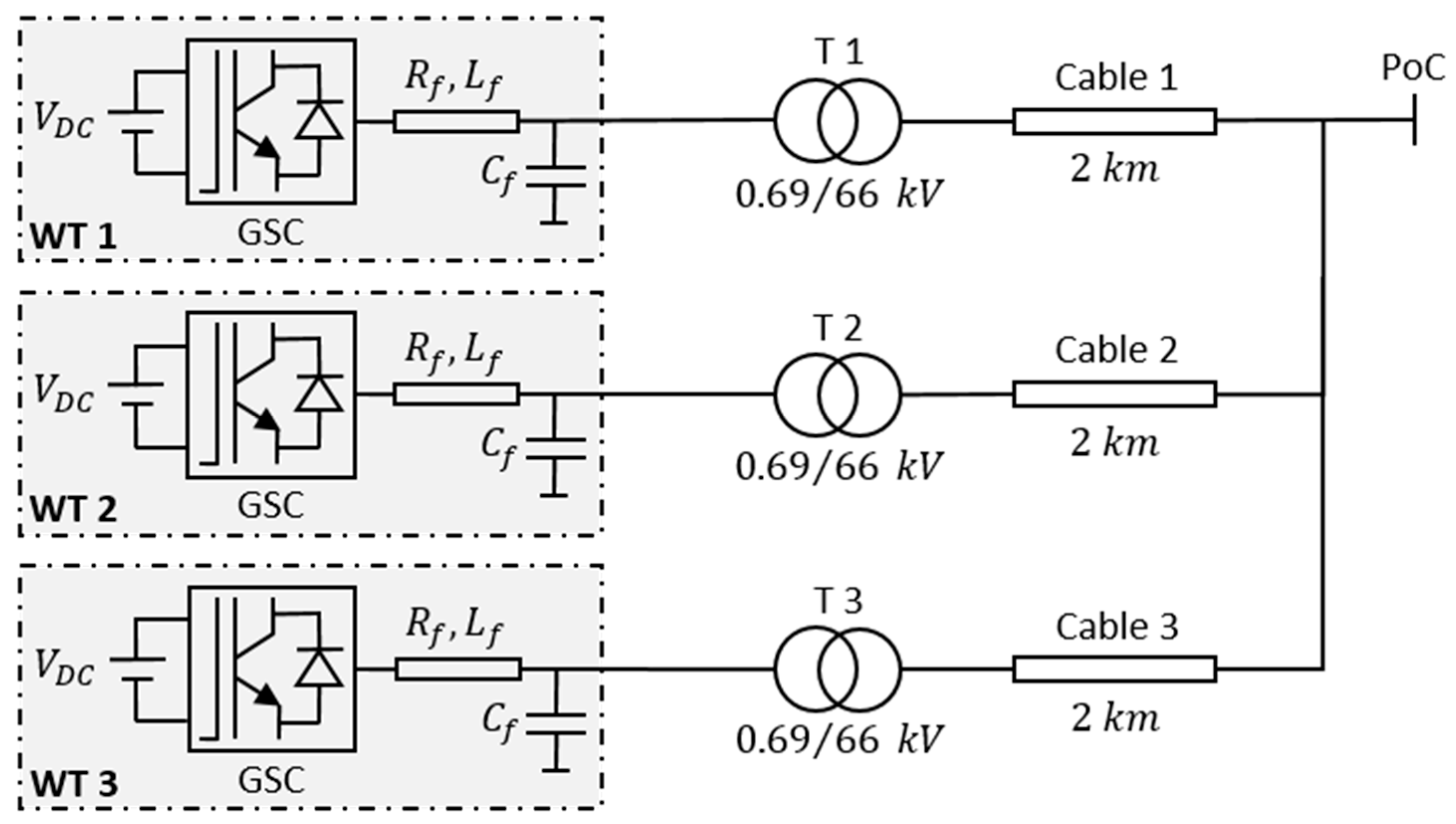
As the discussion in this work is focused on the system level, WP modeling is necessary. WPs are modeled as 3-machines (WTs) aggregated unit, with a total capacity of
. The terminal voltage of each WT is
. A WT transformer changes the voltage from
to
, at which the collector cables operate. A
collector cable is modeled using a
section and its parameters are included in
Table A1 in the
Appendix A. Each cable connects a WT transformer (parameters given in
Table A2 in the
Appendix A) and the WT behind to the point of connection (PoC) in each WP. The schematic of the WP is shown in
Figure 1.
2.1. Grid-Following Frequency Control Method (GFL-FCM)
A GFL-FCM regulates the active power injection from a WT or WP based on the frequency deviation and RoCoF estimated from the voltage at PoC. Therefore, a frequency estimator, i.e., a PLL is used to estimate the system frequency and RoCoF. The synchronous reference frame PLL (SRF-PLL) with a PI compensator is commonly used in controls of converters [
17]. In addition, incorporating a low-pass filter (LPF) in the loop together with a SRF-PLL helps provide an explicit estimation of RoCoF [
18].
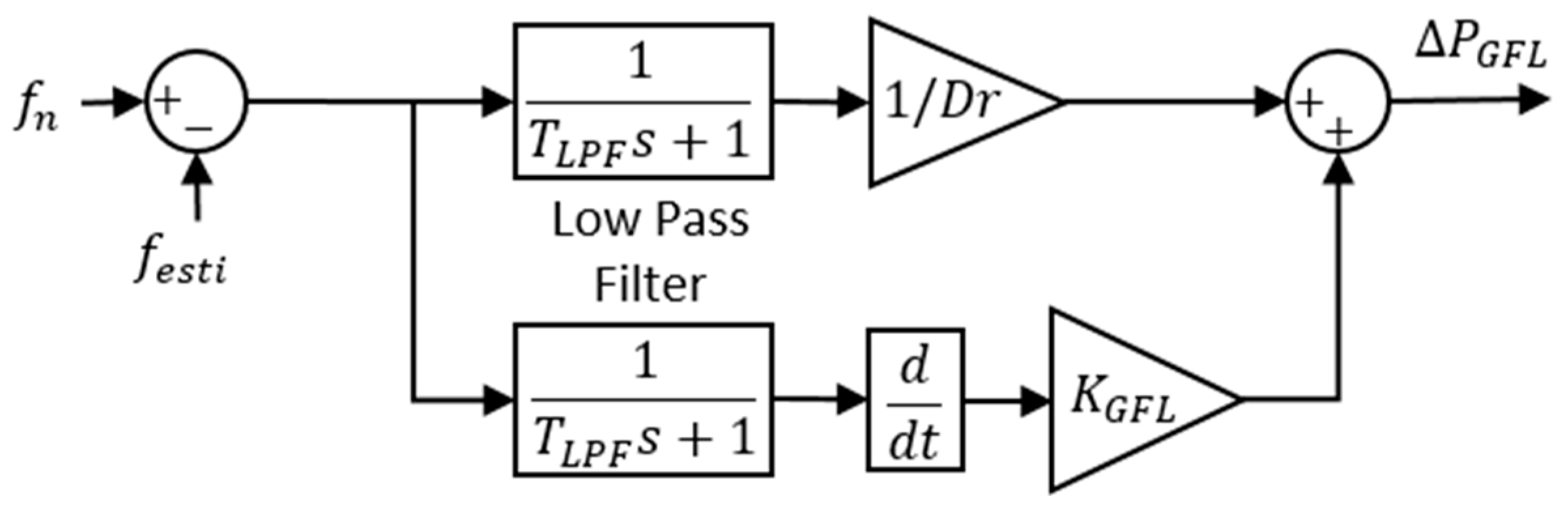
A typical GFL-FCM for offshore wind plants is presented in [
19], and used as a benchmark for comparison with a GFM-FCM. The control scheme is reproduced in
Figure 2.
In this control scheme, is the nominal system frequency. is the estimated system frequency from a PLL. The difference between and is the frequency deviation , which is filtered by a low-pass filter (LPF). The time constant for both LPFs is 2.
After the LPF, the upper branch in
Figure 2 represents the
droop control of the GFL-FCM.
is the droop coefficient, set to
in this work. The lower branch represents the virtual inertial response of the GFL-FCM, which is proportional to the derivative of the frequency deviation
.
is chosen to be 13 under the premise that the controls are in per unit, i.e.,
,
and
are all in per unit. With this value, the best frequency support performance (using metrics such as RoCoF and nadir of frequency) is achieved without inducing high frequency oscillations in the active power output
and without breaching the over-current capability of the WT converters.
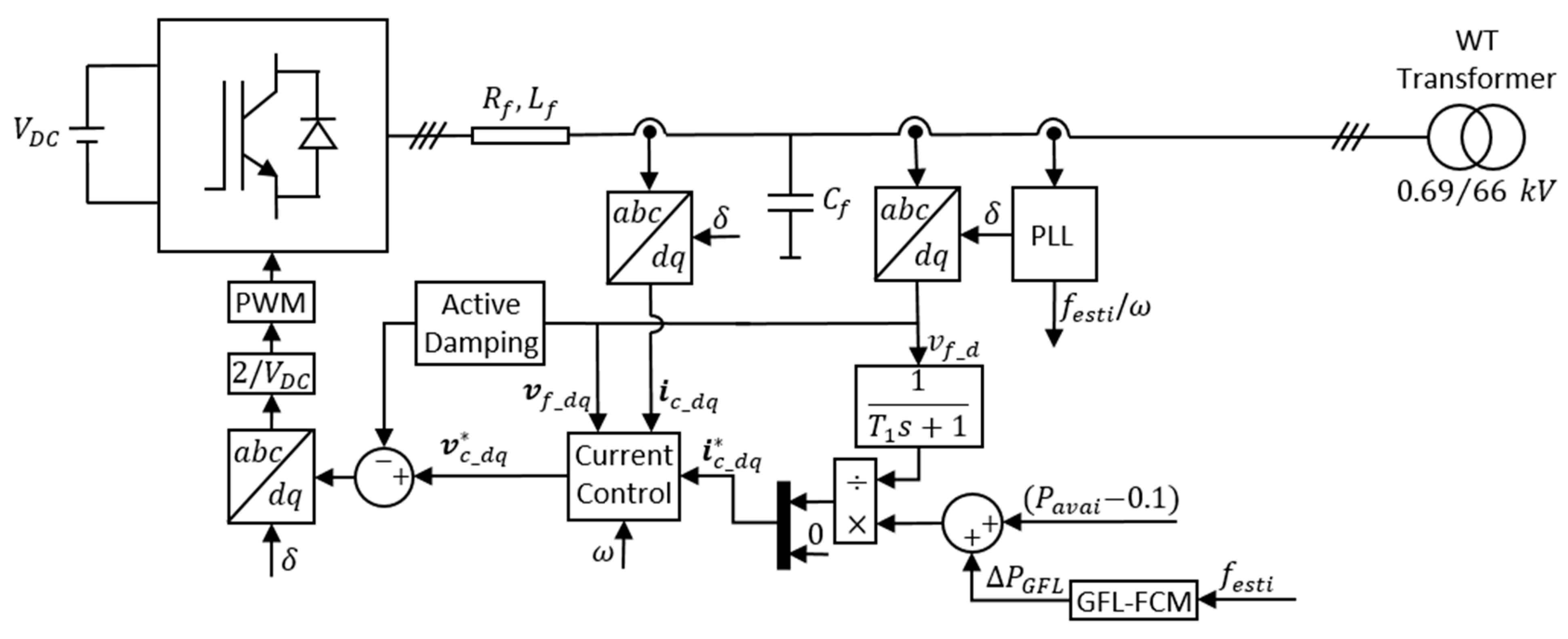
The active power components from the droop control branch and the virtual inertia branch together make up the overall active power that is used for frequency regulation. is added to the normal active power reference for each WT. In this work, we assume all WTs have available power of but operate in a curtailed way, reserving 10% of their nominal power. Hence, the active power reference for each WT is .
With the GFL-FCM implemented, the control scheme of the GSC in WTs is shown in
Figure 3. The parameters are given in
Table A4 in the
Appendix A.
2.2. Grid-Forming Frequency Control Method (GFM-FCM)
An SG can regulate the terminal voltage and system frequency by its excitation and governor respectively. This kind of voltage and frequency control capability is termed as grid-forming (GFM). There are different control methods that all lie in the scope of GFM control [
20].
A reduced-order-VSM-based frequency control scheme is presented in [
21]. It provides satisfactory
droop control and virtual inertia with considerable simplicity. Because of its simplicity, it contains essential elements of VSM control while excluding features that are unique to different realizations of VSM control in the literature [
22,
23,
24,
25]. Therefore, the control scheme in [
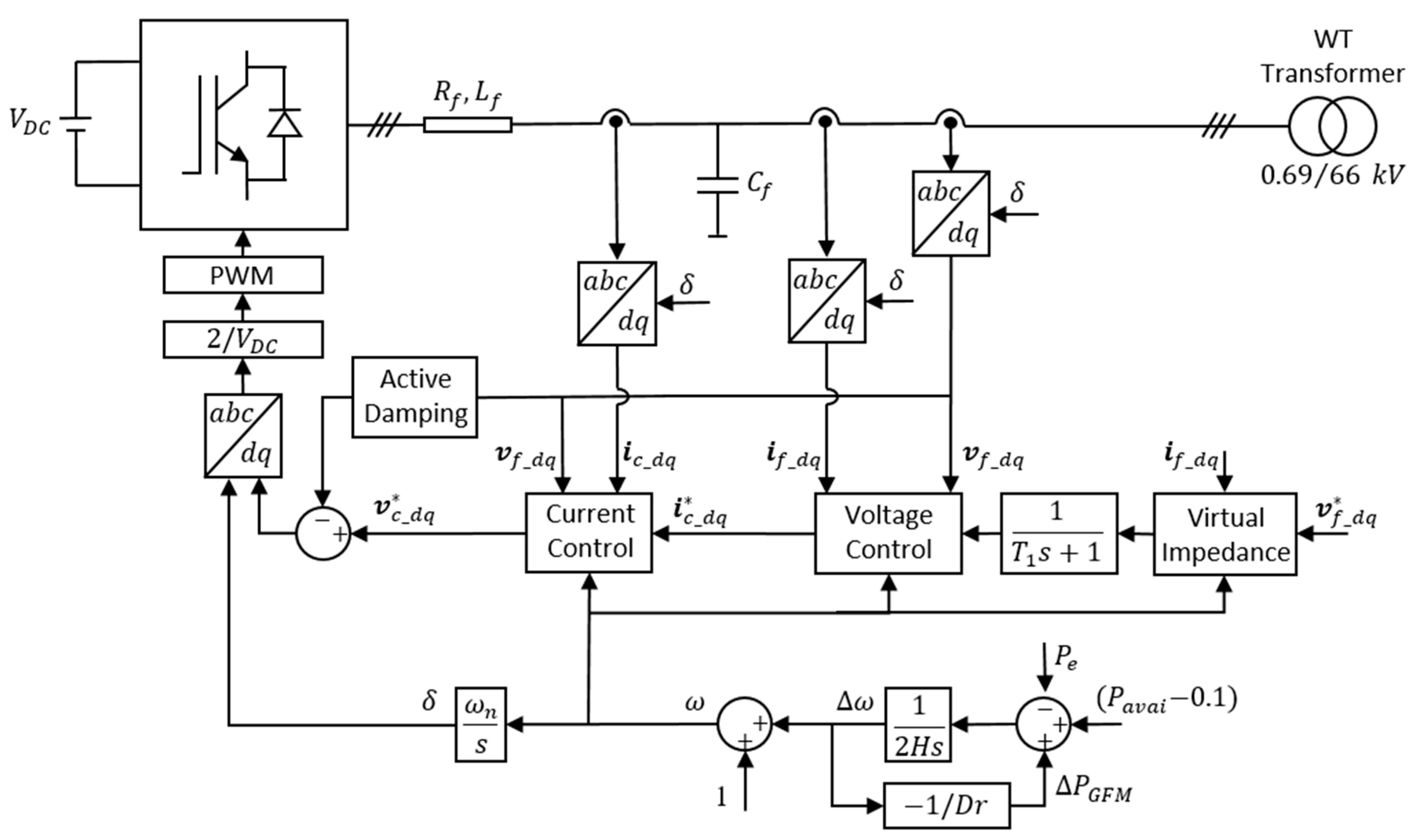
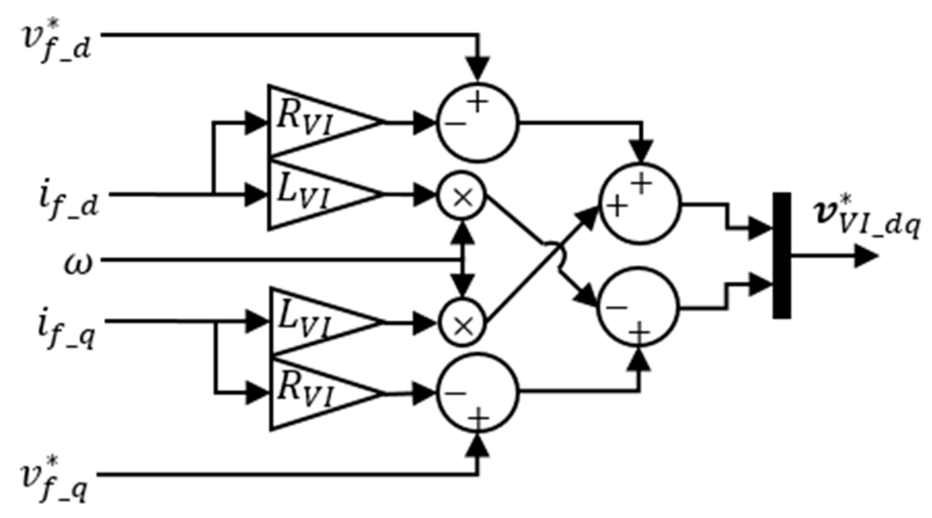
21], as a typical VSM control scheme, is considered as the GFM-FCM in this work, with the addition of a virtual impedance, facilitating parallel operation. The block diagram of the GFM-FCM implemented on each WT is shown in
Figure 4 below. The droop coefficient
is the same with that in the GFL-FCM, which is
. The inertia constant
is kept at
in this work. The values of the remaining parameters are in
Table A4 in the
Appendix A.
The block diagram of the virtual impedance is shown in
Figure 5.
is
, and
is
.
3. Comparison of the GFM-FCM and GFL-FCM on FFR
In this section, we compare the influence of GFM-FCM and GFL-FCM on fast frequency response (FFR) from WPs. In this work, FFR is defined as the same fast frequency response that needs to be delivered in the fast frequency reserve product [
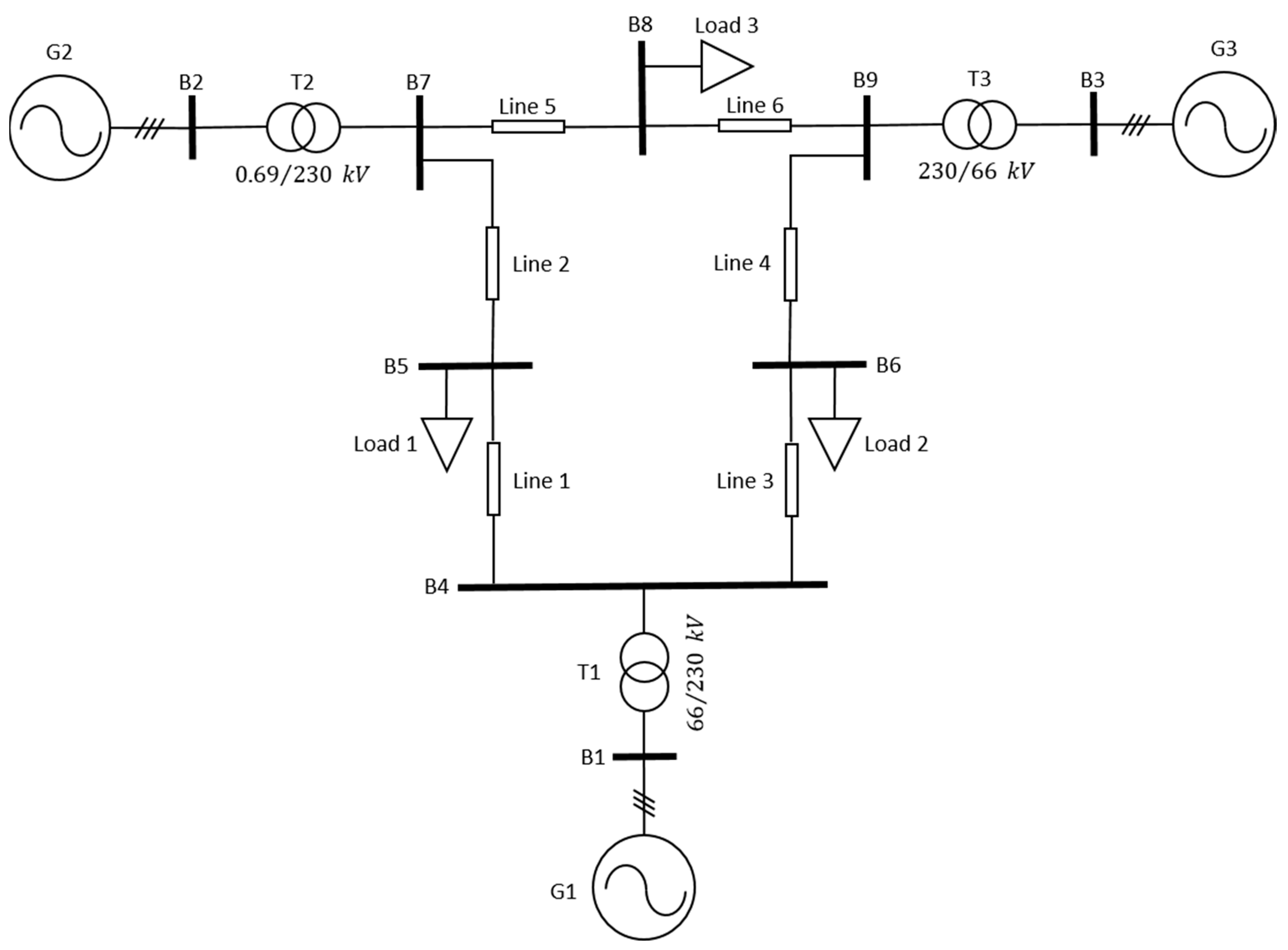
26], in terms of technical properties (activation, duration, etc.). The comparison is tested in the benchmark WSCC 9-bus system [
27,
28,
29]. The topology is shown in
Figure 6. The parameters of the passive components (transformers and lines) can be found in
Table A3 in
Appendix A.
There are three power plants in the system;
is a conventional thermal power plant (TPP),
and
are two WPs that have the same configuration, as shown in
Figure 1. The difference between them is the control mode. In the following simulations, three scenarios are considered. The first is that both WPs are controlled in GFL mode; the second is that
is a GFL-WP whereas
is a GFM-WP; and the third scenario is that both are GFM-WPs. It each scenario, the same frequency event is tested. Therefore, the GFL-FCM and GFM-FCM described in
Section 2 are compared in the same system in the second scenario. More significantly, these three scenarios show how the system frequency stability is developing when GFL-WPs are gradually replaced by GFM-WPs.
As mentioned in
Section 2, for the two WPs
and
, each consists of three WTs and each WT has a capacity of
. Hence, each WP has a capacity of
. For simplicity, the thermal power plant
has the same capacity as each WP, and the three loads are equal in the active power consumption. The parameters of the TPP can be found in
Table A6 in
Appendix A.
An under-frequency event is simulated to check the frequency response of the system. Initially, all three power plants are operating at
of their nominal power, and the WPs have a 10% reserve used for frequency support in an under-frequency event. The event happens at
, when each load is increased by
(equal to 10% capacity of each power plant). The load increase is equally shared by the three power plants as they have the same droop coefficient
. Therefore, for each power plant, their active power output is supposed to increase by
, from
to
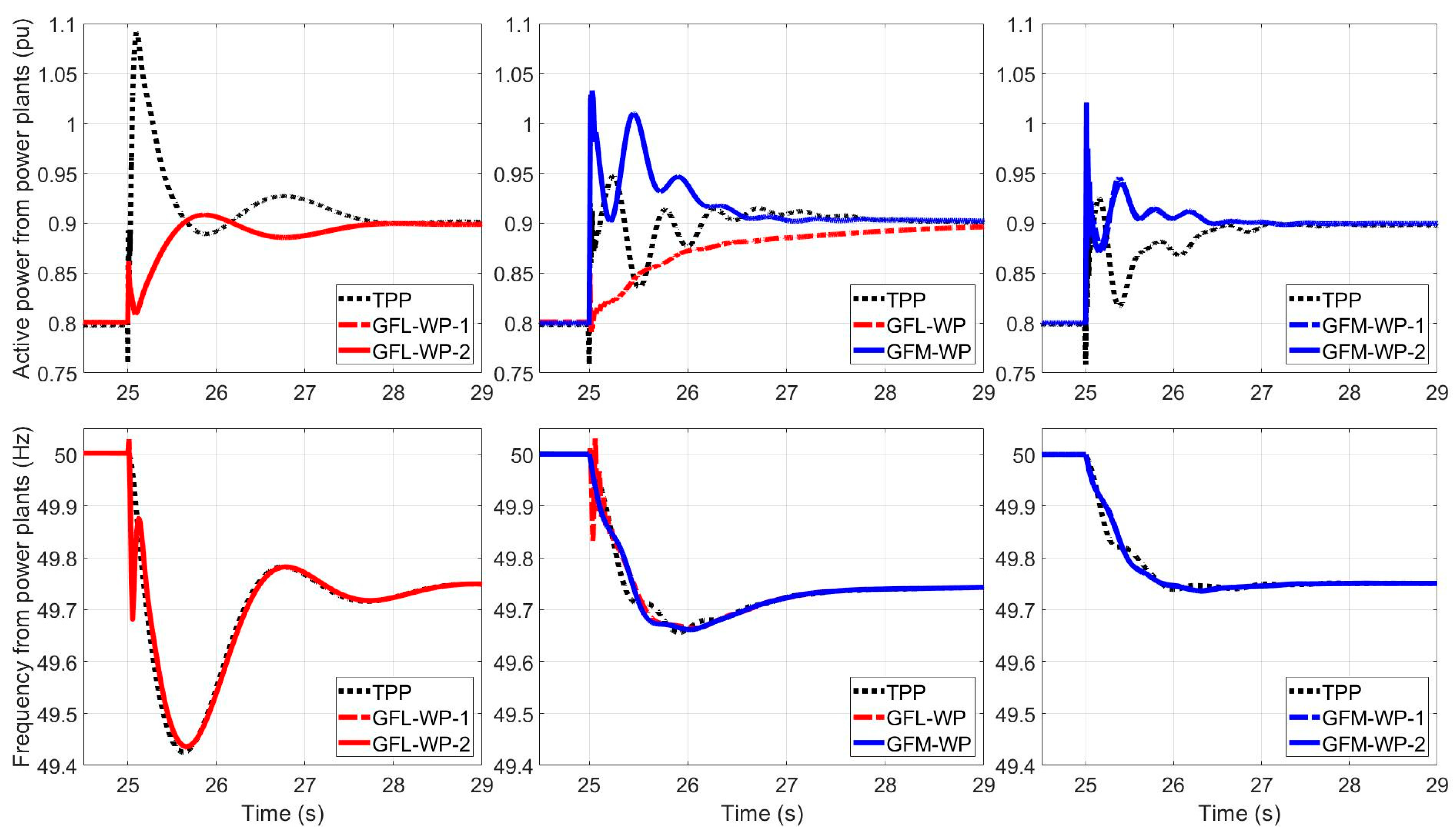
. The results of this frequency event for the three scenarios considered are shown in
Figure 7 and
Figure 8.
The three columns in
Figure 7 represent the three scenarios respectively. In all three scenarios,
is unchanged, which is the thermal power plant in
Figure 6, whereas
and
are varied in the three scenarios: (i)
and
are GFL-WPs; (ii)
is a GFL-WP while
is a GFM-WP; (iii)
and
are GFM-WPs.
The first row in
Figure 7 is the active power output from the three power plants after the under-frequency event
. The second row depicts the corresponding grid frequency in each scenario for the same frequency event. Each subfigure plots of the grid frequency are estimations at these power plants. For the thermal power plant
, the rotating speed of the SG is used as an estimation for the grid frequency. For a GFL-WP, the estimated frequency comes from the PLL. For a GFM-WP, the estimated frequency is the internal frequency within the GFM controller in each WT (
in
Figure 4).
The first row shows the active power outputs after the frequency event, starting on the left with the system with one TPP and two GFL-WPs. As there is a virtual inertial response included in the GFL-FCM, at the beginning of the event, the GFL-WPs are able to provide an instantaneous active power support, which is around in this event of load increase. However, this instantaneous active power support tends to be just a pulse; the active power outputs from GFL-WPs drop instantly close to the pre-event level after the pulse and then gradually increase. On the contrary, the TPP provides a much larger active power support, which is more than 25% of its capacity, immediately after the event because of its inherent inertia. More importantly, though gradually decreasing after the peak, this extra power persists above for half a second before reaching the same level as those from GFL-WPs. Therefore, we might conclude that, in the first half second after the frequency event, which can be considered as the (virtual) inertial response period, the main contributions for frequency support come from the TPP instead of the GFL-WPs. After the (virtual) inertial response period, all three power plants contribute to the frequency support by outputting their active power at , as a consequence of the droop control implemented in them. In addition, low frequency (around ) interactions are observed in active power between the TPP and GFL-WPs. These two WPs have almost the same responses in this event.
In the middle subfigure of the first row, three distinct curves represent the active power response from three different types of power plants in the system. In this scenario, the GFM-WP replaces the TPP and takes the main responsibility for the instant power support at the moment of the event. The instant power support rises up to more than 20% of its capacity. It needs to be addressed that, in this work, no current limitation is considered for the GSCs in WTs. Furthermore, we assume the WPs have a 10% reserve in active power, which is meant for the extra power output in the steady state after the event, for example,
in
Figure 7. Hence, the extra part of their power output in the first second after the event, which is beyond the 10% reserve, needs to be supplied from somewhere else. An energy buffer, either a super-capacitor or battery, at the DC-link is able to fulfil the task, but this aspect is out of the scope of this work. A DC voltage source is connected at the DC-link for all the WTs (as shown in
Figure 1,
Figure 3 and
Figure 4), which provides the possibility of any amount of extra power from WTs.
If we still consider the first half second as the (virtual) inertial response period, in this stage, the main contributions for frequency support come from the GFM-WP and the TPP. The GFM-WP has an even larger contribution than the TPP in terms of the velocity of action and the amount of power. The former might be due to the rapidity of converters, which is an obvious advantage of GFM-WPs in FFR. For the GFL-WP, its power output at the instant of the event is very similar to that in the subfigure on the left, which increases and decreases almost at the same time (). It is also a pulse of around , but it is overlapped by the blue curve in the middle subfigure. Afterwards the GFL-WP slowly increases its active power from pre-event set-point to post-event steady state . Because of the droop control implemented in all three power plants, they all contribute equally in compensating for the load change. In this scenario, low frequency (around ) interactions are observed in active power from the TPP and the GFM-WP.
The subfigure in the upper right corner gives the results of active power responses in the system with the TPP and two GFM-WPs. The initial responses are very similar to those in the middle subfigure. The GFM-WPs contribute more than the TPP in the momentary overshoot of power at the starting of the event. This is because virtual inertial response is inherent in the GFM-FCM by emulating the swing equation of SGs. Although inertial response is inherent in SGs, it seems that the virtual inertial response from a GFM converter behaves faster and stronger than the inertial response from the mechanical rotating mass of an SG, under the circumstances that both of them have the same (virtual) inertial constant values. This is thanks to the rapidity of power electronic devices and their electronic controllers, which possibly turns out to be an advantage of GFM IBRs over traditional TPPs in maintaining the power system stability. As a GFM-WP is contributing more than a TPP in the early stage of FFR (around after the event, including the virtual/real inertial response period) and there are two GFM-WPs in this scenario, the TPP is contributing less in this early stage than that in the second scenario (the middle subfigure). Similar interactions in active power, such as those in the second scenario also exist from the TPP and GFM-WPs in the third scenario. All three power plants share the same load increase in the post-event steady state due to the same droop coefficient values in their controls. In general, from the second and third scenarios, we can conclude that GFM controls enable a WP to achieve behaviour (FFR in this case) that is more dominant than that of a TPP.
In the second row are the results of the system frequency. The frequency curves are derived at each power plant, with its own estimation method. As GFL-WPs rely on PLLs to estimate the system frequency, drastic changes in the frequency values are observed at the origin of the event in the first two subfigures (from left to right). This illustrates the transient process in the PLL to track the frequency. These drastic changes in frequency estimation bring challenges in calculating the RoCoF and introduce disturbances to the control system. This could be considered as a drawback of using PLL in FFR. In addition, there are also some minor mismatches between the frequency estimations from the TPP and GFM-WPs in the early stage of FFR (around after the event). In steady state, all the frequency estimations are identical as it is a global variable. However, the most important part is the nadir of the frequency, and the results show a clear improvement when GFM-WPs are gradually replacing GFL-WPs in the system.
To have a clearer and more direct comparison of the three scenarios, we plot the system frequency of the three scenarios in the same figure (
Figure 8). The frequency estimation from the rotating speed of the SG is used as the indicator of the system frequency for all three scenarios.
The improvements—both for the frequency nadir and for the RoCoF—are very clear, leading to the conclusion that by replacing a GFL-WP with a GFM-WP, both the nadir of frequency and the RoCoF are improved in an under-frequency event.
Furthermore, to compare these three scenarios horizontally both in
Figure 7 and
Figure 8, it is also easy to draw the conclusion that by replacing a GFL-WP with a GFM-WP, it takes less time for the system to go through the transients and to reach a new steady state after the frequency event.
4. Conclusions
In this paper, we mainly compare two different frequency control methods from wind turbines and plants: grid-following and grid-forming control. Two control schemes of these two types of controls are introduced, implemented and compared in a WSCC 9-bus system. Three scenarios of system configurations are simulated and compared, in which grid-following and grid-forming controlled wind power take different shares in pre-event power output and post-event frequency support. This gives an insight into how the frequency stability of power systems changes as grid-forming wind plants gradually replace grid-following ones.
Grid-following and grid-forming frequency control methods present rather different frequency support response in active power output from wind plants. With virtual inertial response implemented in the frequency control method, grid-following wind plants could provide instantaneous power support at the instant of the frequency event, but this power output cannot sustain long, being almost just a pulse, especially when coexisting with other grid-forming units (SGs or GFM-WPs) in the system. The magnitude of the pulse is also quite limited. Hence, grid-following frequency control methods in fact cannot contribute much in the virtual inertial response period, in which grid-forming units take the main responsibility. Overall, in the whole frequency support process (from the beginning of the event to the post-event steady state), grid-following wind plants behave just like ‘followers’. By saying so, we mean, they are not as active as grid-forming units in their ability to quickly and largely increase the power output to make up the power imbalance. On the contrary, grid-following wind plants increase power output at a slow pace and gradually reach the steady state with no or little overshoot. Partly this is due to the dominant role of grid-forming units in frequency and voltage controls.
In contrast, grid-forming wind plants show very similar behavior as synchronous generator-based power plants in frequency control, which is very beneficial for maintaining the system frequency stability while at the same time increasing the wind power penetration in the system. More importantly, grid-forming wind plants demonstrate even more dominant behavior in the frequency support context than thermal power plants, due to the rapidity in response of power electronic devices compared to slow dynamics in rotating machines. This indicates a potentially promising popularization of grid-forming IBRs and their contributions to forming a reliable 100% inverter-based power system.
From the comparison of the three scenarios, by replacing a grid-following wind plant with a grid-forming one, the system frequency undergoes less severe RoCoF and higher nadir in an under-frequency event. This illustrates the superiority of grid-forming frequency control methods over grid-following ones. This also suggests a roadmap towards increasing wind power penetration further in the system while maintaining or even improving the system’s frequency stability.


