Dynamic Lyapunov Machine Learning Control of Nonlinear Magnetic Levitation System

Abstract

This paper presents a novel dynamic deep learning architecture integrated with Lyapunov control to address the timing latency and constraints of deep learning. The dynamic component permits the network depth to increase or decrease depending on the system complexity/nonlinearity evaluated through the parameterized complexity method. A correlation study between the parameter tuning effect on the error is also made thus causing a reduction in the deep learning time requirement and computational cost during the network training and retraining process. The control Lyapunov function is utilized as an input cost function to the DNN in order to determine the system stability. A relearning process is triggered to account for the introduction of disturbances or unknown model dynamics, therefore, eliminating the need for an observer-based approach. The introduction of the relearning process also allows the algorithm to be applicable to a wider array of cyber–physical systems (CPS). The intelligent controller autonomy is evaluated under different circumstances such as high frequency nonlinear reference, reference changes, or disturbance introduction. The dynamic deep learning algorithm is shown to be successful in adapting to such changes and reaching a safe solution to stabilize the system autonomously.

1. Introduction

Deep learning is a multi-layer technique for shallow machine learning that enables the neural network to learn complex nonlinear patterns. While a single-layer neural network can make approximate outcome predictions, the addition of hidden layers improves prediction accuracy. Over the last few years, the integration of deep learning into industrial applications has progressed in areas such as robotics, self-driving vehicles, healthcare, and renewable energy. Researchers have advanced the integration of deep learning and nonlinear controls, enabling the controller to successfully learn control policies and iteratively arrive at approximate solutions via reinforcement learning [1]. Other researchers have concentrated on the use of machine learning to gain insight into the unknowns associated with complex system dynamics [2].

While deep-learning-based cyber–physical systems have a number of advantages, such as the ease with which complex patterns may be detected, ability to adapt and learn towards unknowns, and a higher degree of accuracy of predicting the outputs compared to shallow neural networks, but they also present a number of downsides. For instance, DNNs places a premium on the accuracy and diversity of the data collection in order to produce objective findings. Additionally, DNNs make no guarantees about the safety or feasibility of a proposed solution or its conclusions [3]. The introduction of additional data to the DNN addressed the set bias issue, it imposed a delay in the time required for the DNN to identify the best approach [4]. One of the major challenges of DNN in CPS presented in [5] is also finding the right balance between deeper architectures and practical regularization approaches. Linear and nonlinear controllers have presented a practical solution to low to mid-complexity static systems. Despite being efficient in managing mid-complexity system behaviors, they become susceptible to high complexity cyber–physical systems [6]. The control Lyapunov function (CLF) has been employed successfully to control complex nonlinear duffing and Van der Pol systems [7,8,9]. The idea behind using nonlinear controllers allows for a lossless control strategy to avoid system linearization while the integration of deep learning allows for the continuous adjustment and selection of system and control parameters. Machine learning has been utilized in previous research along with usually what is described as a cost function, but one of the downsides found was the amount of time required for the DNN to relearn during the process of updating the data set and also the time requirement to come up with the appropriate solution [10,11]. Further, as demonstrated in [12], the DNN accuracy and run-time to find a solution was affected by the number of parameters required and the dataset size.

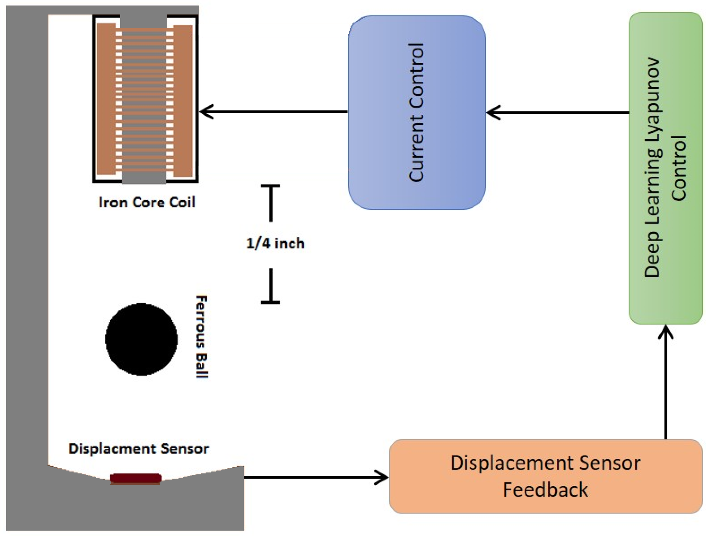
Magnetic levitation has emerged as a feasible solution to the present demand for quicker and more efficient transportation methods, and its contact-free technology is already finding uses in space and military in addition to allowing for high speed, safe transit alternatives to railways. For the feedback control loop in a magnetic levitation system, position, velocity, and acceleration measurements are obtained. After the necessary signals have been measured and processed, they are fed into a feedback loop. To measure position, velocity, and acceleration in a Maglev system, contactless transducers must be used. Position and accelerometer sensors are employed to gather system data. Broadband, stability, and robustness in all working situations, linearity over the operational ranges, noise immunity, and immunity to radiation and stray magnetic fields all go into the selection of the transducer. Magneto-optical transducers are made up of two coils wrapped around a nonmagnetic rod. To activate the primary coil, which generates the magnetic field that creates an eddy current, an alternating current must be applied to it. When the eddy current passes through the secondary coil, it forms a magnetic field that generates voltage. The output of the secondary coil decreases as the track gets closer to the secondary coil, due to an increase in the opposing eddy-current field. The output of the transducer may be monitored using Lyapunov nonlinear control, and the clearance between the object and the rails can be regulated. Since batteries have a limited amount of power and are used in both present and future transportation applications, efficiency has been one of the most important design factors. The Maglev system in [13,14,15] incorporated energy harvesting or energy scavenging, which is the technique of capturing and converting ambient energy into useful electrical energy. Various energy sources have been effectively recycled during the last decade, including wind, solar radiation, thermal radiation, vibrations, and, most recently, magnetic energy harvesters. Coils, actuators, and a controller are all necessary components of magnetic energy harvester systems in order to collect and govern the recovered energy. There are coil-magnet components in the harvester that utilize Faraday’s law of electromagnetic induction [16].

CPS systems will continue to grow in complexity following a trend of growth in technology and microchips. The National Academies journal has stated in 2016 that: “today’s practice of CPS system design and implementation is often ad hoc and unable to support the level of complexity, scalability, security, safety, interoperability, and flexible design and operation that will be required to meet future needs”. While previous literature in [17,18] focused on toggling the control law between two or more options through machine learning. In addition, several assumptions or utilizing machine learning are used to utilize the control law over multiple iterations. In this research, we realize that computational solutions such as deep learning have some limitations when it comes to time constraints [10]. This research introduces the use of Pearson correlation and prioritizing high correlation parameters to the error within the algorithm. Moreover, we focus on the utilization of parameterized complexity to evaluate the dataset and keep the depth of the NN to a minimum while maintaining accurate output. A custom architecture of layers is presented. To the best of our knowledge, the integration of the previously mentioned concept has not been discussed in previous literature.

In this research, a novel approach is developed based on the parameterized complexity theory to estimate the complexity of the dataset and accordingly change the depth of the DNN. Rather than quantifying the system complexity purely in terms of its input length, other numerical properties of the input instance are considered such as the correlation between the dataset parameters collected while the CPS system is running or the memory occupation increase or decrease. The initial data set is a collection of parameter variations and their effects on the output. An updated dataset is collected via the deep neural network (DNN), and runs based on the initially defined CPS information. We identify high-performance compact deep learning architectures through a neural architecture search and meta learning. The neural network architecture is customized to minimize the training time and computational power required. A new data set is recorded if the delta error between the actual system error and the predicted system error generated by the DNN after the substitution with the proposed parameters is greater than 0.4. The system begins to add to its current data set while keeping in memory 40% of the older data set. A novel function to calculate the number of NN layers required to relearn the parameters tuning effect on the model. In addition, a novel control Lyapunov function is presented and the results are compared to a PID-controlled Maglev system from [19]. The proposed controller is shown to successfully stabilize the system under different disturbances and reference signal changes safely without going into an infinite loop.

2. Materials and Methods

Due to its efficiency and wide range of applications in real life, the study of magnetic levitation devices has been a focus in both the industrial and long-term theoretical research fields. As more Maglev applications are launched, additional control modifications will be required to ensure the system’s stability.

In this section, a traditional Magnetic Levitation system plant model is explored and the system dynamics equations are presented [20] and then the energy harvesting portion of the model dynamics is introduced [21].

The nonlinear model can be represented by the following set of differential equations and is schematically shown in Figure 1.

2.1. Magnetic Levitation System Dynamics

Traditional magnetic levitation model:

$$m\ddot{x}-\sigma \dot{x}=\frac{i^2{k}_c}{{(x-x_0)}^2}-m_{k}g$$

(1)

m: mass of the ball.

g: gravity.

x: displacement.

ẍ: acceleration.

i: current.

$\sigma$: damping constant [N/m.s].

The displacement and current position of the ball in the magnetic field is controlled by electric current supplied and governed by Equation (2).

$$F_s=\frac{I\left(t\right)}{U\left(t\right)}=\frac{k_a}{T_s+1}$$

(2)

i(t): current at time t.

U(t): voltage at time t.

$K_a$: coil inductance.

$T_s$: time constant.

Energy harvesting magnetic levitation model:

$$x+mg+x{K}_{ma{g}_b}-K_{ma{g}_t}+S\dot{q}+(c_m+c_e)\dot{x}=0$$

(3)

m: mass of the ball.

g: gravity.

x: displacement.

ẍ: acceleration.

i: current.

Alpha: magnetic force constant.

The system in Equation (3) presents a traditional magnetic levitation system dynamics. The displacement sensor will provide the feedback needed for the Lyapunov deep learning control to determine the appropriate control signal.

$$L_s\ddot{q}+R_s\dot{q}+\frac{q}{C_s}-S\dot{x}=ecos\left(\omega t\right).$$

(4)

v: voltage input.

R: resistance.

L: inductance.

2.2. State Space Representation

The below state space equation is aimed towards controlling the position of the Ferrous ball. Taking

$$x_1=Displacement,x_2=Velocity,x_3=i$$

(5)

therefore, Equations (4) and (5) can be written as a matrix format while considering position as output.

$$\left[\begin{array}{c}\dot{x_1}\\ \dot{x_2}\\ \dot{x_3}\end{array}\right]=\left[\begin{array}{c}{x}_2\\ g-\frac{\alpha }{m}{\left(\frac{x_3}{x_1}\right)}^2\\ -\frac{R}{L}{x}_3+\frac{2\alpha }{L}\frac{x_2{x}_3}{x_1^2}\end{array}\right]+\left[\begin{array}{c}0\\ 0\\ \frac{1}{L}\end{array}\right]$$

(6)

$$y_{Position}=\left[\begin{array}{ccc}1& 0& 0\end{array}\right]$$

(7)

A variation in the y matrix is made to change the intended controlled output.

$$y_{Velocity}=\left[\begin{array}{ccc}0& 1& 0\end{array}\right]$$

(8)

$$y_{Current}=\left[\begin{array}{ccc}0& 0& 1\end{array}\right]$$

(9)

2.3. Design of the Lyapunov Controller

Lyapunov control has proven successful in managing complex nonlinear oscillators to a certain extent of oscillator frequency $\omega$ = 2.5 Hz [7]. In order to improve the system stability at a higher $\omega$, deep learning was introduced in [4]. The deep learning algorithm is taught the relationship between the system parameters change, the controller parameter change, and the output error slope. If the algorithm detects a sudden change in slop a parameter update is triggered and the deep learning algorithm substitutes the current parameters with updated parameters that are expected to bring the system to stability.

The application of control Lyapunov functions was developed by Z. Artstein and E. D. Sontag in the 1980s and 1990s. Control Lyapunov functions are utilized to determine the stability of a system or a system ability to regain stability. A control Lyapunov function u is selected such that the function is globally positive definite and the time derivative of the control function $\dot{u}$ is negative definite and globally exponentially stable.

$$u=\frac{1}{2}{(\dot{e}+\alpha e)}^2$$

(10)

taking the time derivative of u

$$\dot{u}=(\dot{e}+\alpha e)(\ddot{e}+\alpha \dot{e})$$

(11)

$$\dot{u}=(\dot{e}+\alpha e)((\ddot{y_d}-\ddot{y})+\alpha \dot{e})$$

(12)

such that the error e = $y_d-y$. $y_d$ is the desired state and y is the actual state. Upon substitution in $\ddot{y}$ in (12) we obtain the control law U. The Lyapunov function for the system in (1) is derived for the magnetic levitation model as

$$U=\frac{km}{2}(\dot{e}*\alpha e)+\alpha \dot{e}m+gm+K_{f}v\dot{x}-\frac{i^2*K_c}{{(x-x_o)}^2}+\ddot{y}m$$

(13)

The Lyapunov function for the system in (3) is derived for the energy harvesting magnetic model as

$$U=-\ddot{y_d}-{\alpha }_4\ddot{y}-{\omega }_{4}y+{\alpha }_3\frac{\ddot{x}+x+{\omega }_3{x}^3+{\alpha }_2\dot{y}}{-{\alpha }_1}-Ncos\left(\theta t\right)-\alpha \dot{e}-\frac{k}{2}(\dot{e}+\alpha e)$$

(14)

2.4. Deep Learning Algorithm

The research completed in [7] revealed that the controller parameters had substantial impact on the desired system outcome and error; therefore, the research in [4] successfully presented a deep learning approach that would allow 1 of the controller parameters to change while the system is operational thus tackling sudden changes in stability. One of the disadvantages found through the survey in [10] is that the system learning/relearning process robustness is significantly reduced if more parameters require updates simultaneously. Thus to reach system stability the time requirement and computational cost would significantly increase due to the large variations in the data in the data set. Since the updated parameters are not found within the target time, the system would fail.

In this paper we present a deep learning approach aided by different methods to alleviate the timing issue in research [11] and to increase the number of parameters that can be changed while maintaining a timely outcome and system stability. Researchers have proven success in utilizing the Lyapunov stability function in dynamic DNN weights [22] but in this research the number of deep learning layers increase or decrease in proportionality to the dataset complexity. The controller parameters that fall under the deep learning network include $k,\alpha ,k_{fv},k_c,{\alpha }_3$. The parameters were selected by measure of effect on the controller signal and desired output.

Recently, optimization has become popular for finding network architectures that are computationally efficient to train while still performing well on certain classes of learning problems [23,24,25], leveraging the fact that many datasets are similar and thus information from previously trained models can be used. While this strategy is frequently highly effective, the current disadvantage is 11 certain works, for example [26], place a greater emphasis on the model’s memory footprint reduction. The overhead of meta learning or neural architecture search is computationally intensive in and of itself, since it needs training several models on a diverse collection of datasets, while the cost has been dropping in recent years approaching the cost of traditional training.

A critical constraint for learning is the size of the data set used to train the original model. For instance, shown that picture recognition performance is strongly influenced by image biases and that without these biases, transfer learning performance is reduced by 45%. Even with unique data sets created specifically to imitate their training data, we observe an 11–14% decrease in performance [27]. Another possibility for circumventing deep learning’s computational limitations is to switch to other, maybe undiscovered or undervalued methods of machine learning; therefore, in this research we integrated several methods to circumvent the data complexity relationship to computational cost.

2.4.1. Custom Deep Learning Architecture

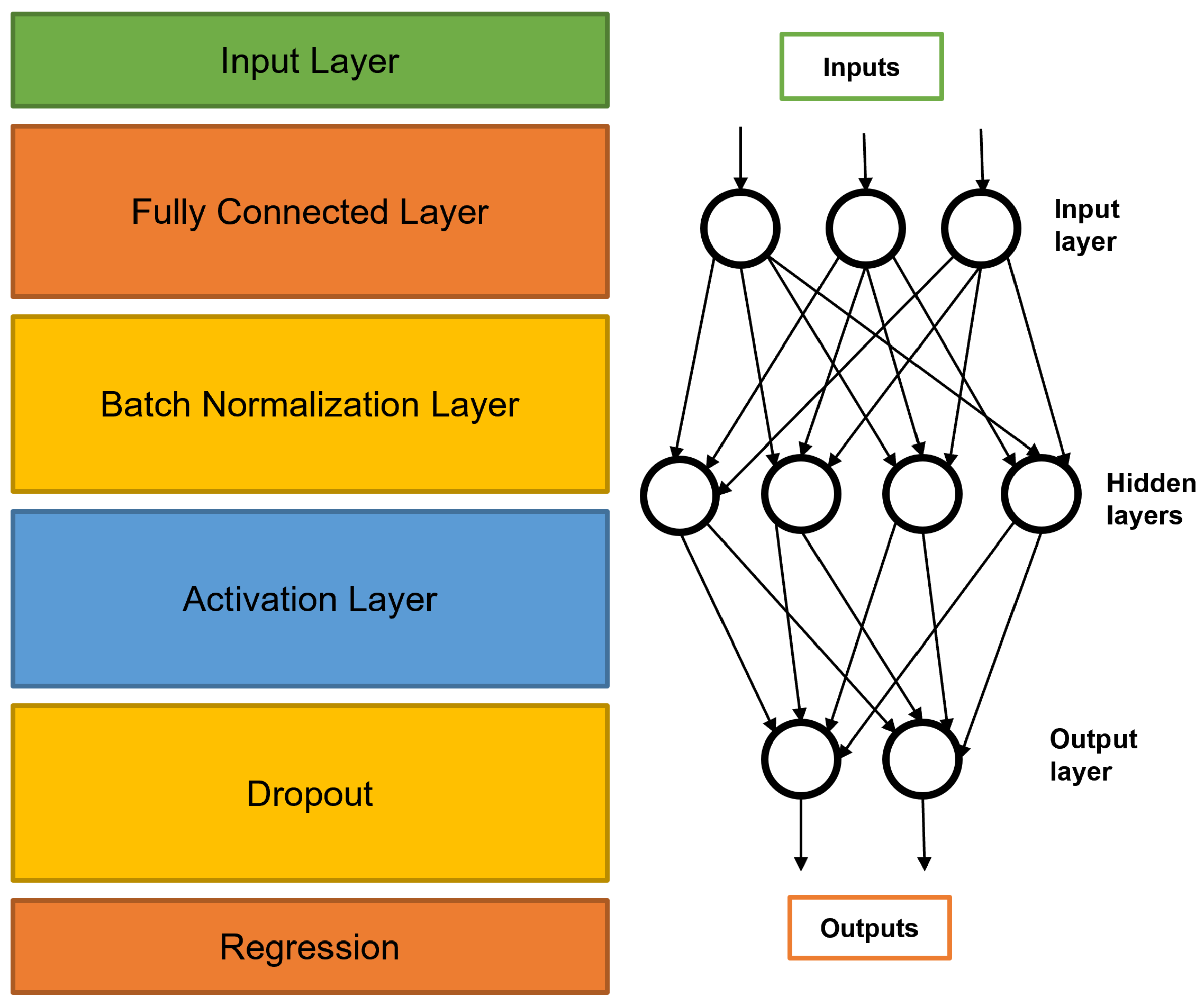
The network architecture begins with the input layer receiving a precollected data set of 38,000 points including the time, V (cost function), velocity, position, parameters ($k,\alpha ,k_{fv},k_c,{\alpha }_3$), reference, and error. Secondly, we create a convolution layer to compute the correlation between the input data sets. A fully connected convolution layer reduces the losses in correlation in contrast to a regular convolution layer. The third layer is a batch normalization layer to stabilize the learning process and reduce the number of training epochs required to train the network. The forth activation layer is required to stabilize the learning process and reduce the number of training epochs required to train deep networks. A fifth dropout layer is introduced to resolve the problem of over-fitting. Over-fitting occurs when the networks have high accuracy on the training data set but very low accuracy on the test data set. Finally the regression layer is added to compute the losses and readjust the node weights to accordingly. Algorithm 1 presents the steps towards obtaining the output.

Algorithm 1: Dynamic Deep Learning Algorithm.

Memory = 40% of the old training data previous_system_average = system error average of the training data initialization;

2.4.2. Parameterized Complexity and Dynamic Programming

The goal of parameterized complexity is to provide an alternate way for resolving intractable computational problems [28]. Rather than defining the complexity of an algorithm solely in terms of the length of its input, other numerical features of the input are considered. For example, the vertex cover problem is NP-hard, which means that it is unsolvable in the usual sense. If the run-time is additionally expressed in terms of the vertex cover size k, this problem can be solved in time 2O(k)nO. If k is small enough in comparison to the number of cases to solve, this is referred to as tractable. This improved concept of efficiency is called fixed-parameter tractability, and it has evolved into a canon of computational complexity [29]. Dynamic programming breaks down a complex problem into smaller decision sub-problems. These usually contain overlapping values that can be adjusted, but more crucially, the local values can be blended in a controlled fashion. Value functions are typically indicated by the notation V1, V2, …, Vn, where Vi signifies the system’s value at step i. Typically, the procedure involves some type of recursion [30,31]. Following this reasoning we define the complexity of our data set using two factors. factor K is the number of data points, As the number of data-points increases the assumed dataset complexity increases proportionally. On the other hand factor f is defined as the number of parameters or features defined in the data set, as the correlation increases the relationship between the parameter and controlling the error is easier to ascertain. According to the above assumptions, the relationship $O\left(kfnLog\right(n\left)\right)$ was utilized. For the case of having 38,000 data-points where K is the constant $2.8\times {10}^{-4}$ and 7 features, it would yield 37 min of estimated DNN run time. At 6 min of run time it was found that 5 deep learning layers delivered 97% accuracy; with the increase in the required run time for each additional 10 min of run time, one additional layer was added. For 100,000 datasets, for 17 min of run time we added one additional fully connected convolution layer with 50 nodes increasing the number of deep neural network layers to 6 layers while maintaining 97% accuracy or higher.

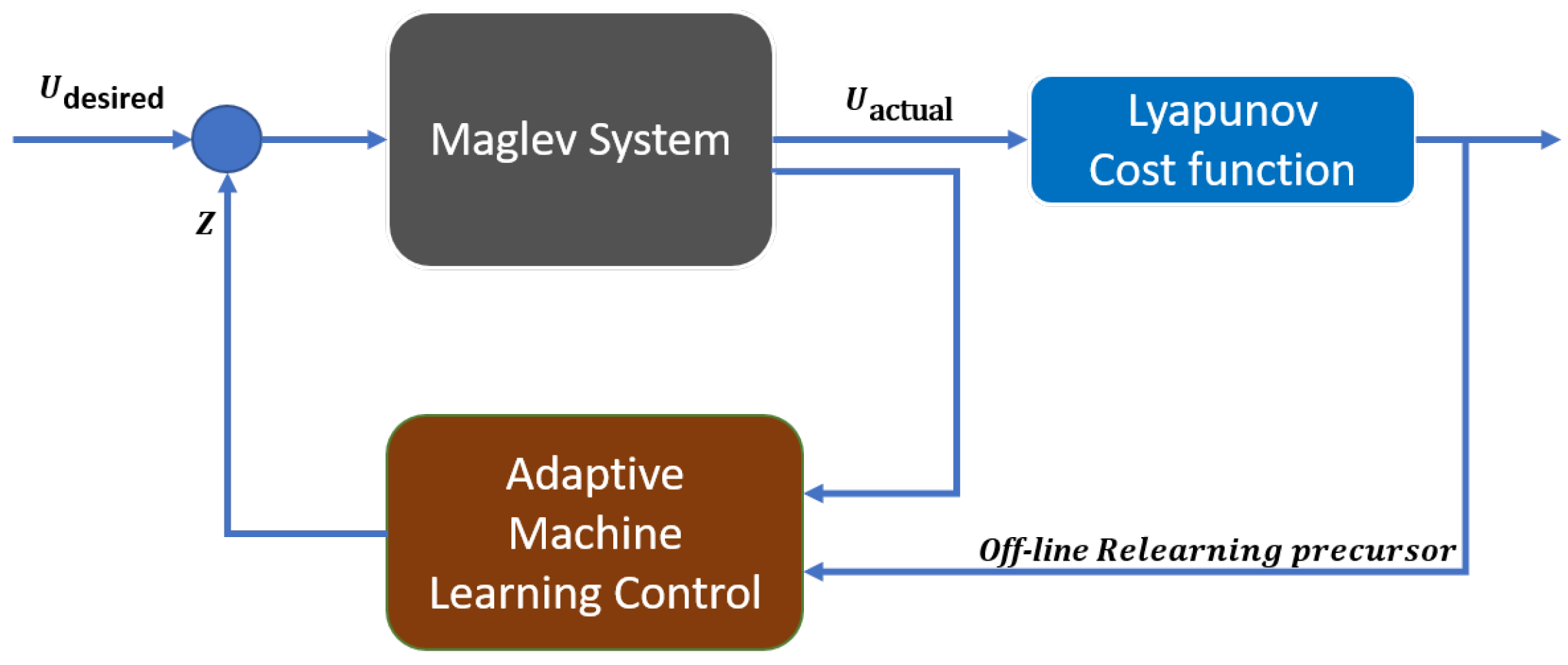
The algorithm flow diagram is presented in Figure 2 to integrate the Maglev system model and Lyapunov control with the DNN running in the background with the continues stream of new data to support relearning. The DNN architecture developed is presented in Figure 3 where 38,000 data-points propagate through the input and hidden layers as the system begins to accumulate new data points. In order to maintain safe control strategy only 10% of the data set is updated when the DNN predicted error accuracy begins degrading. The AI runs continuously in tandem with the control and system. If the error slope surpasses a set threshold > abs|1| the neural network is queried to introduce new control parameters that are predicted to reduce the current system error. The network proposed in Figure 3 is initially trained and then used to predict new ($k,\alpha ,k_{f_v},k_c,{\alpha }_3$).

The concept of memory use is commonly referred to as self-refreshing memory and was first introduced and tested in [32,33,34]. The notion is that even when perturbations occur, they may not stay long enough for the network to lose its ability to anticipate the system error if the system parameters return to normal after the network has been retrained numerous times.

2.4.3. Deep Learning Algorithm Data Set

Initially the model is ran multiple times with different ($k,\alpha ,k_{fv},k_c,{\alpha }_3$) while the output velocity, displacement and error is collected in a time indexed data set. The data set is later used to train the dynamic DNN model, which predicts the error for any suggested set of ($k,\alpha ,k_{fv},k_c,{\alpha }_3$) depending on the current state of the system (velocity, displacement) at time t. The DNN is triggered to intervene if the error slope of 10 sequential data points exceeds the set value of 0.5. The algorithm sequentially begins to suggest an alternative set of control parameters predicted by the DNN to bring the system back to stability. After the suggested parameters are placed in the controller if the error slope does not begin to decline within 5 s from the introduction of new parameters the algorithm restarts the process while in parallel comparing the actual error to the predicted error if the difference is more than 1 then the DNN is triggered to relearn the system dynamics keeping 40% of the old data set in memory to maintain system safety.

3. Results

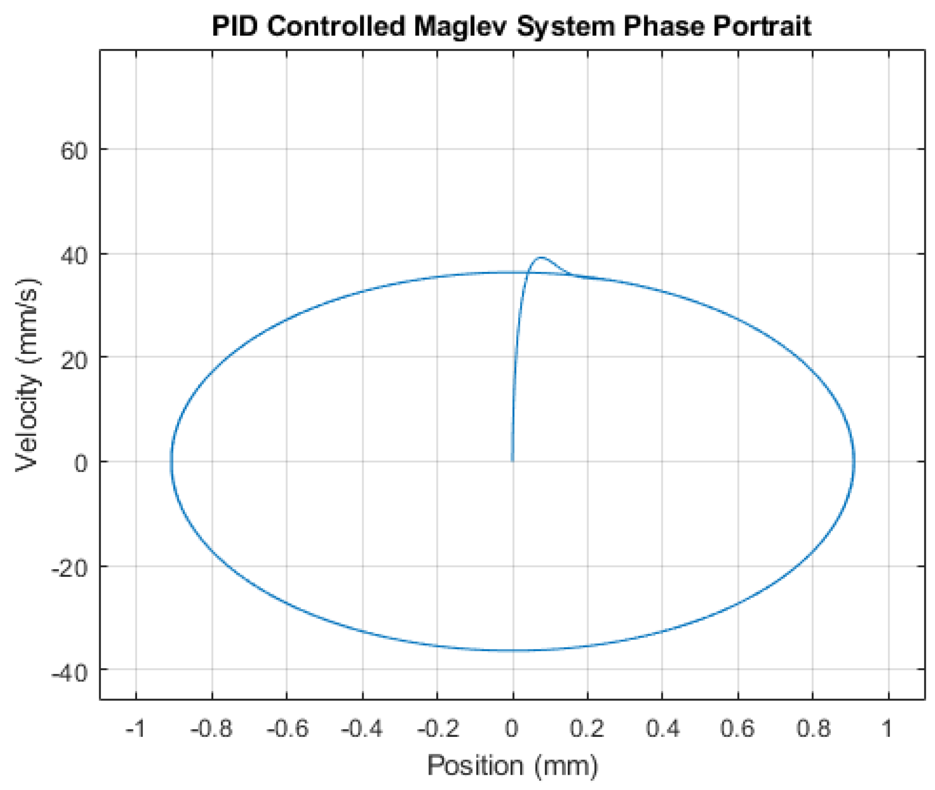
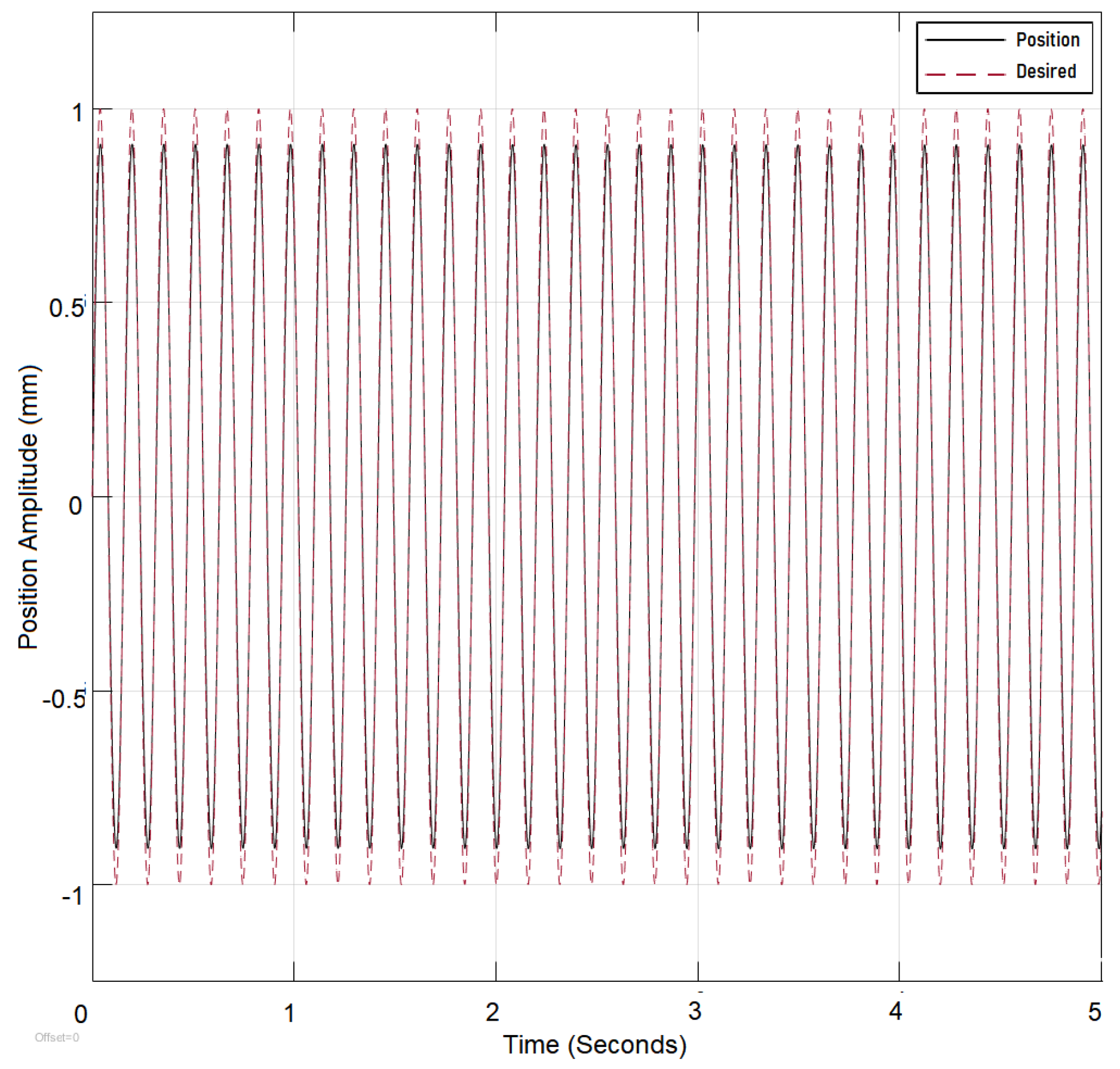
Initially The system is tested without the DNN and with the Lyapunov control in place. The results are compared to a system without the DNN and with PID control in place. Both controllers were tested under an input reference sine wave signal and input frequency of 40 rad/s. The results are recorded as shown in (Figure 4, Figure 5, Figure 6 and Figure 7). The system is found to be stable with the system parameters set to the values in

Table 1. Maglev system parameters.

Parameter	Value
Mass (Kg)	0.1
Gravity ($\frac{m}{s^2}$)	9.8
$R_s\left(Ohm\right)$	1
$C_s\left(F\right)$	0.5
$L_s\left(Henry\right)$	0.4
e	0.002
S	0.4
$\omega$	2

and the controller parameters set to the initial static values in

Table 2. Lyapunov controller parameters.

Parameter	Value
K	0.1
Alpha1	9.8
$K_{fv}$	2
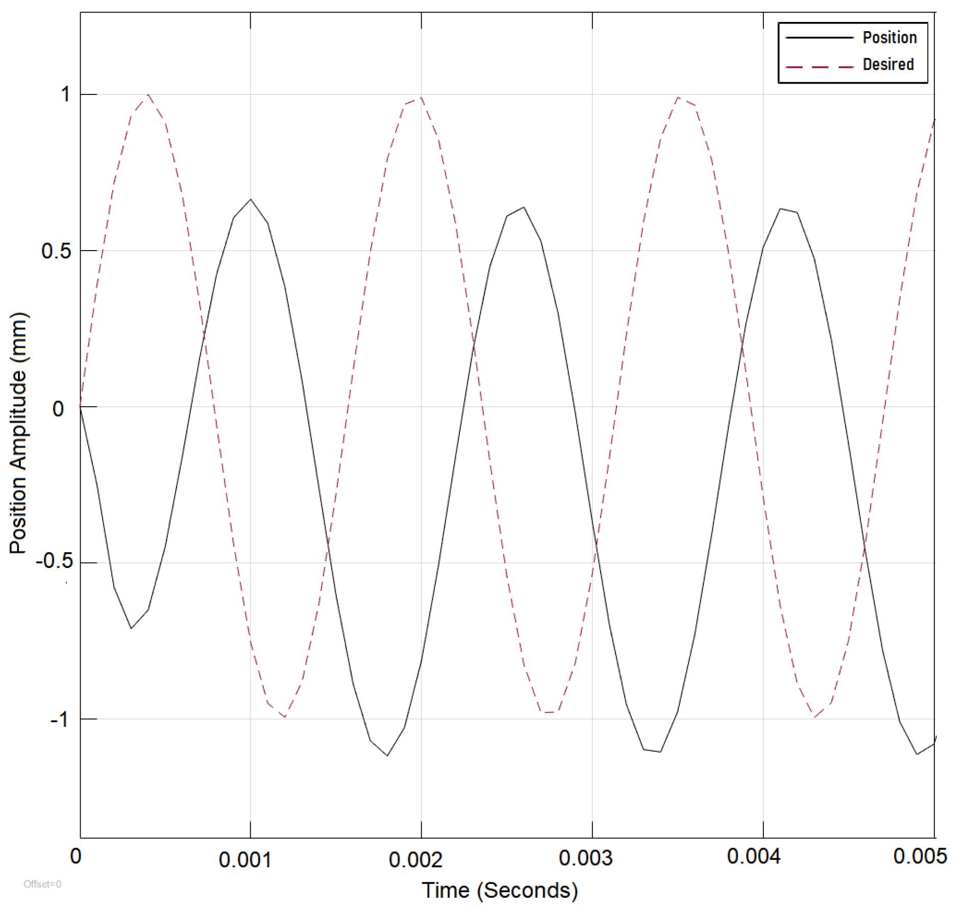
$K_c$	0.001

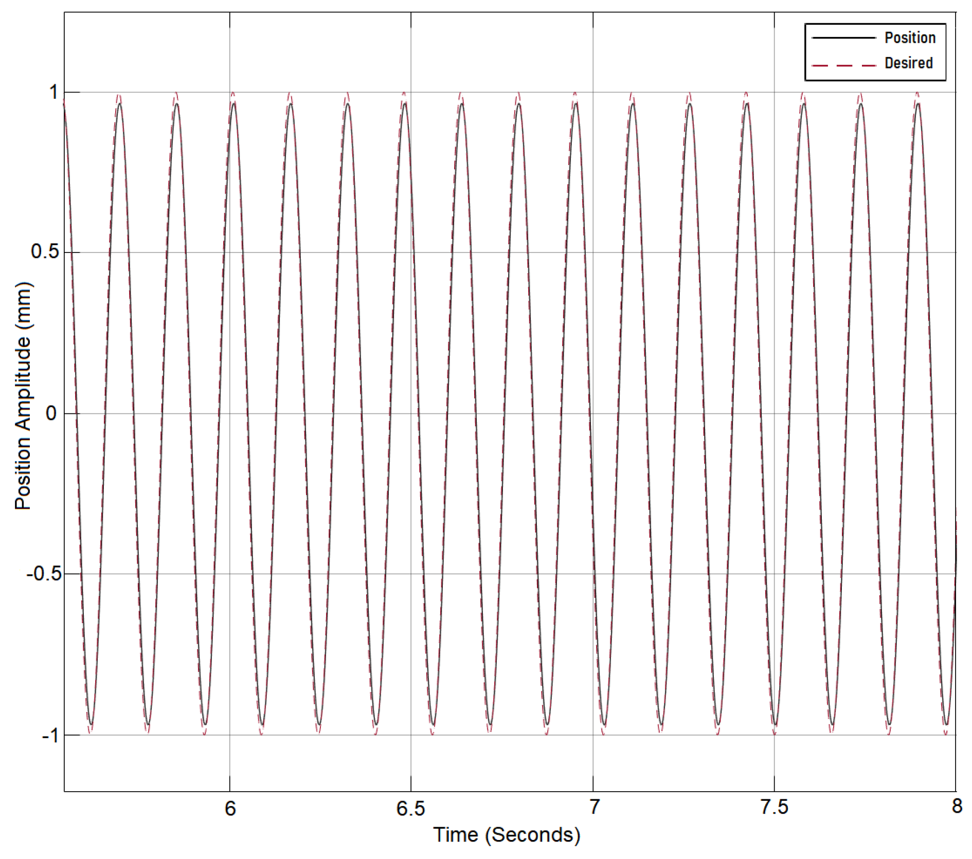
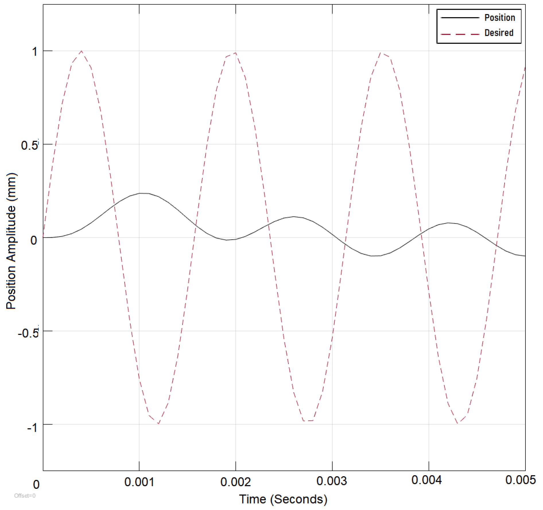
until the $\omega$ frequency of oscillations of the reference signal is increased over 4000 rad/sec where the system error begins to increase and both controllers have shown there static parameters unable to compensate for the change in $\omega$ (Figure 8 and Figure 9). The Lyapunov-controlled system outperformed PID since PID required a choice between overshoot and undershoot. 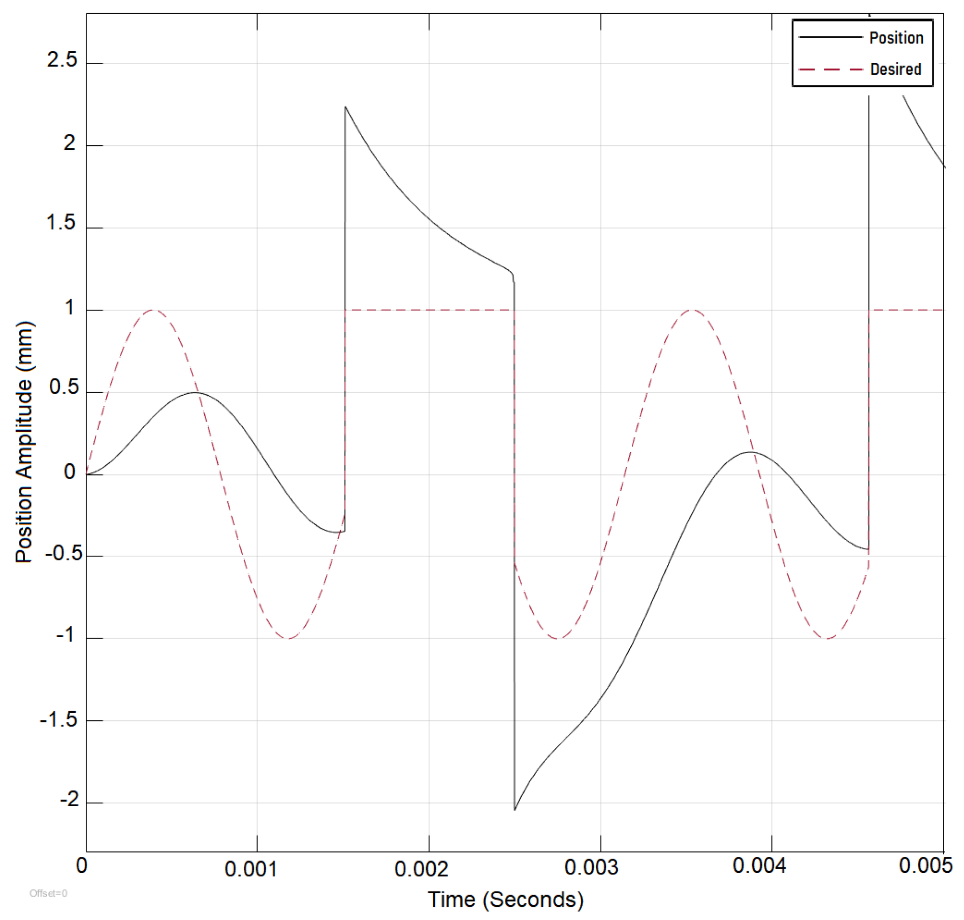The system performance would improve but with an initial overshoot that would repeat with the change of the step value; therefore, Lyapunov control was selected for the adaptation as Lyapunov controller performance is shown to be superior to the PID as shown in Figure 4 and Figure 5. The system was also tested under switching reference signals before the addition of dynamic deep learning and after its addition and the results are recorded to show the improvement. Under switching signal conditions the PID controller is shown to perform less effectively as shown in Figure 10).

Once the desired reference signal is changed from sinusoidal to the step function, the output error increases significantly as the static parameters require some changes to adapt for the signal change. Hence, the application of deep learning resolves sudden changes in the reference signal, as is shown in Section 3.2, where the algorithm reaction to reference signal change is detailed.

3.1. Error Parameter Correlation Study and Deep Learning Algorithm Application Results

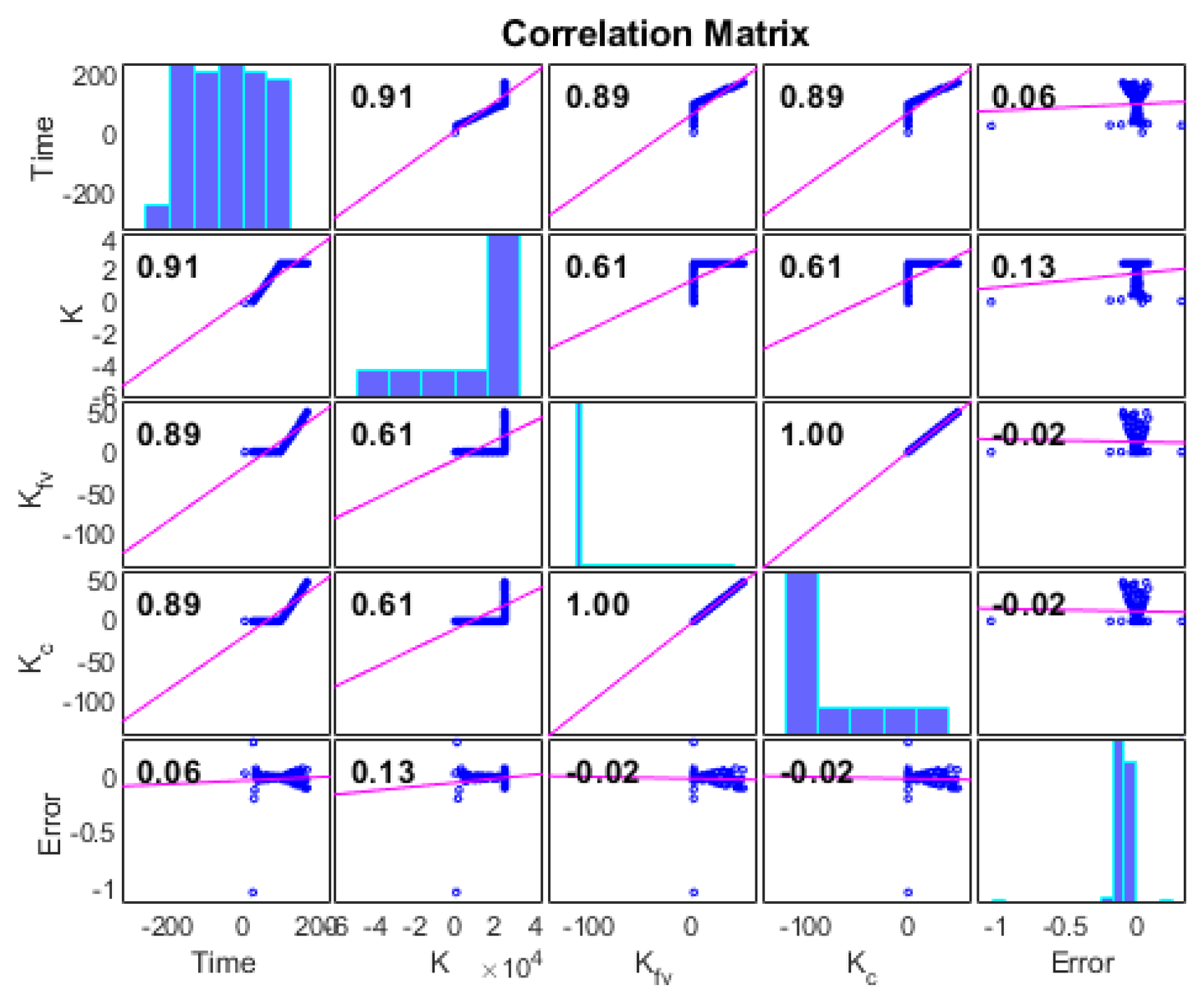
The controller parameters were found to have different effects on the error variation as time progress. It was found that as the dataset is increased from 38,000 points to 100,000 data points and the parameters under the DNN purview are increased from one parameter K to 5 parameters ($k,\alpha ,k_{fv},k_c,{\alpha }_3$) the DNN time required to find the appropriate combination of parameters was infinite; therefore, a Pearson correlation study between the effect of parameter change and error was utilized. The Pearson correlation coefficient (PCC) is a measure of the linear correlation between two sets of data and the results presented in Figure 11. The ratio of two variables covariance to the product of their standard deviations with the result always falling between −1 and 1 was demonstrated by (15). The priority is then assigned to each parameter accordingly. The correlation data are updated with the introduction of a new data set or if the deep learning network is triggered to relearn. The sequence at which the parameters are changed is also studied by varying the parameters in different sequences while the error vector is recorded. It was found that the change of sequence of the controller parameters had no effect on the output error reduction but instead the parameter with the highest correlation to the error had the most impact on the error reduction.

$$r=\frac{{\sum }_{i=1}^n(x_i-\overline{x})(y_i-\overline{y})}{\sqrt{{\sum }_{i=1}^n{(x_i-\overline{x})}^2}\sqrt{{\sum }_{i=1}^n{(y_i-\overline{y})}^2}}$$

(15)

As Figure 11 shows, the highest correlation is between K, and as the error in parameter K is varied, the error is either reduced or increased depending on the state of the system; therefore, the priority of change to control is given to k and then the other parameters sequentially $\alpha ,k_{fv},k_c,{\alpha }_3$. The correlation is continuously calculated as mentioned in the previous paragraph to account for change. In this section, we apply the DNN described in Section 2.4 to observe its effect on the system performance and hence the error. 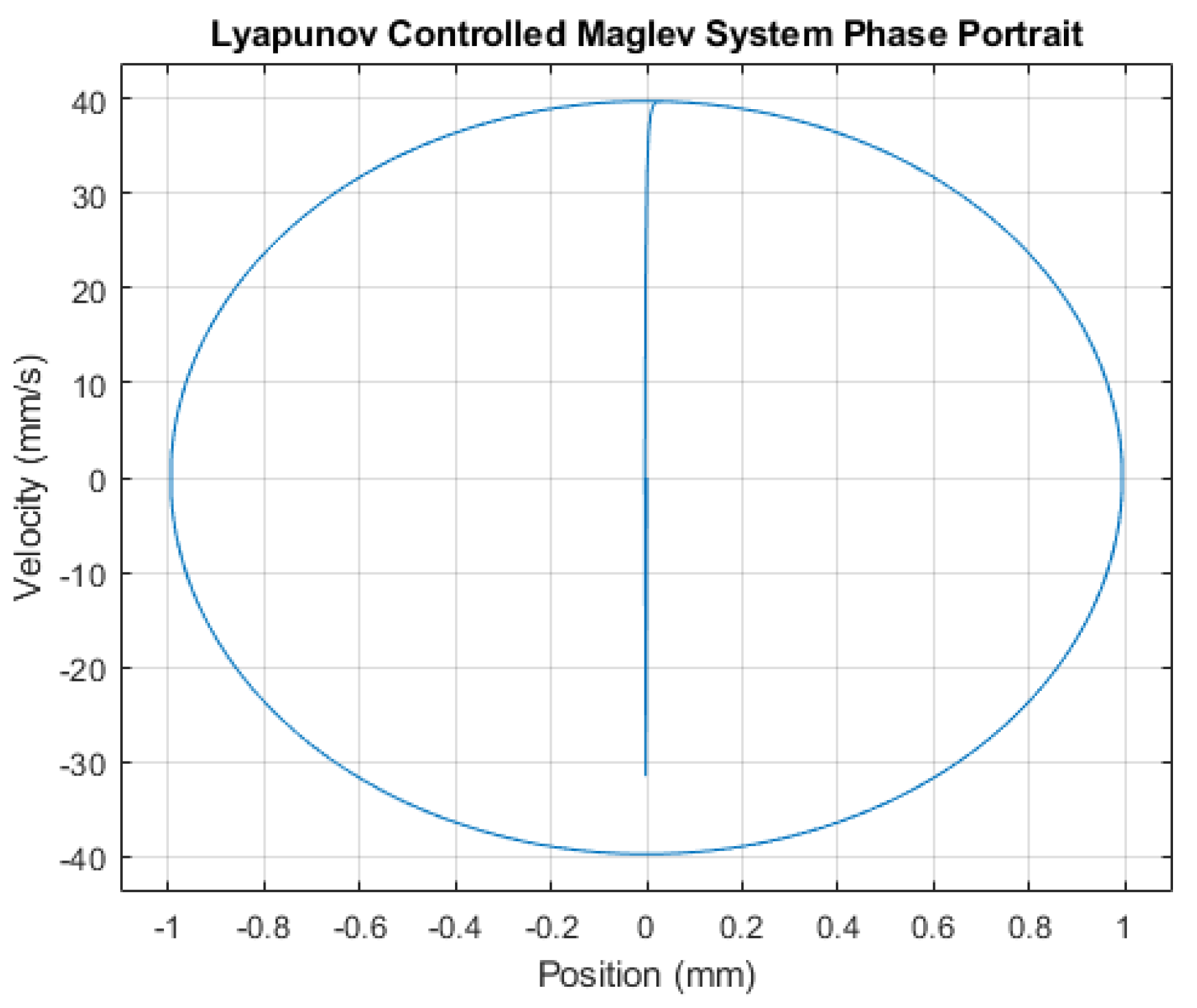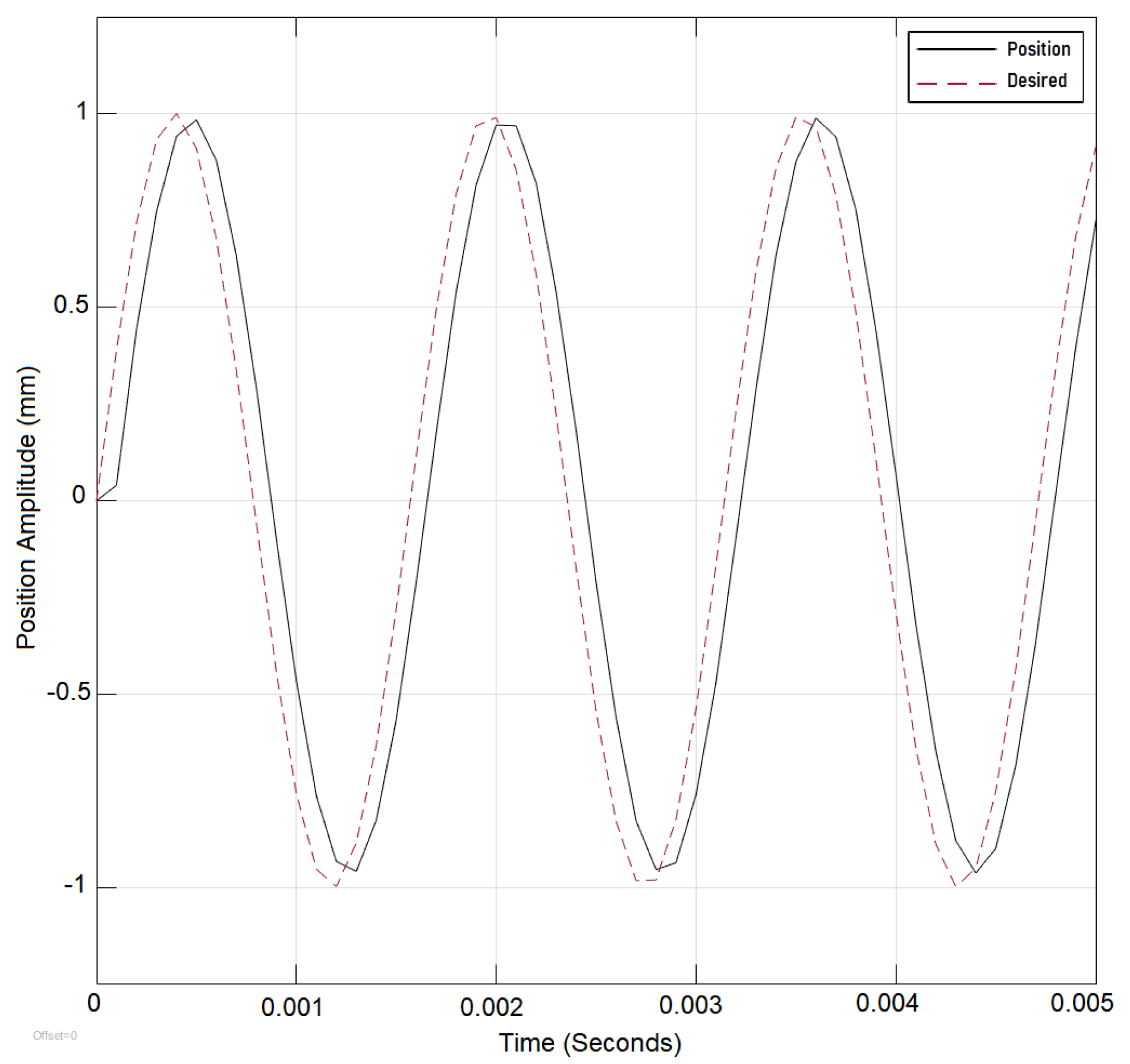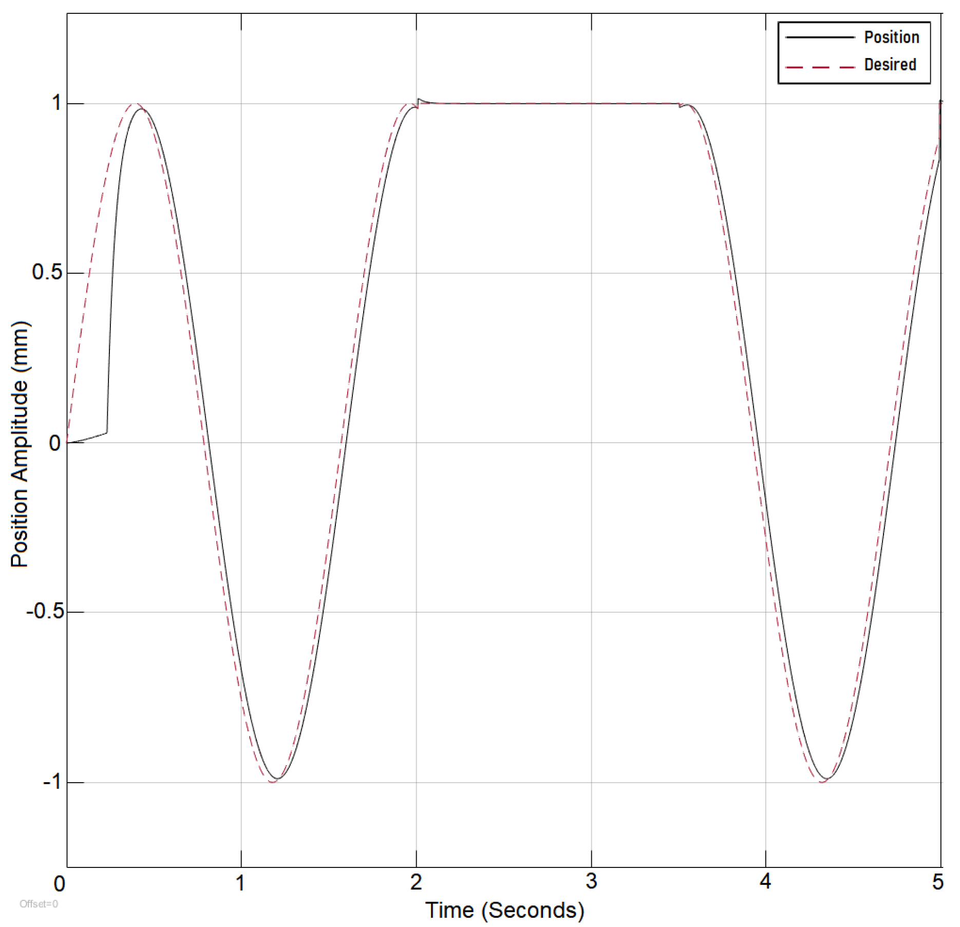Figure 12 and Figure 13 shows the effect of utilizing the Dynamic Lyapunov control in stabilizing the system output under high frequency. In Figure 14, the reference signal is shown to be switched from sinusoidal to the step function and back to sinusoidal with the error between the reference and output position signal successfully being under control. The deep learning network reacts to the change of the reference signal type by updating the controller parameter K to 2700 from 20. If the change of K does not restabilize the system, the algorithm considers the second-highest parameter correlation to the error $\alpha$ and then the third, as mentioned at the beginning of this section.

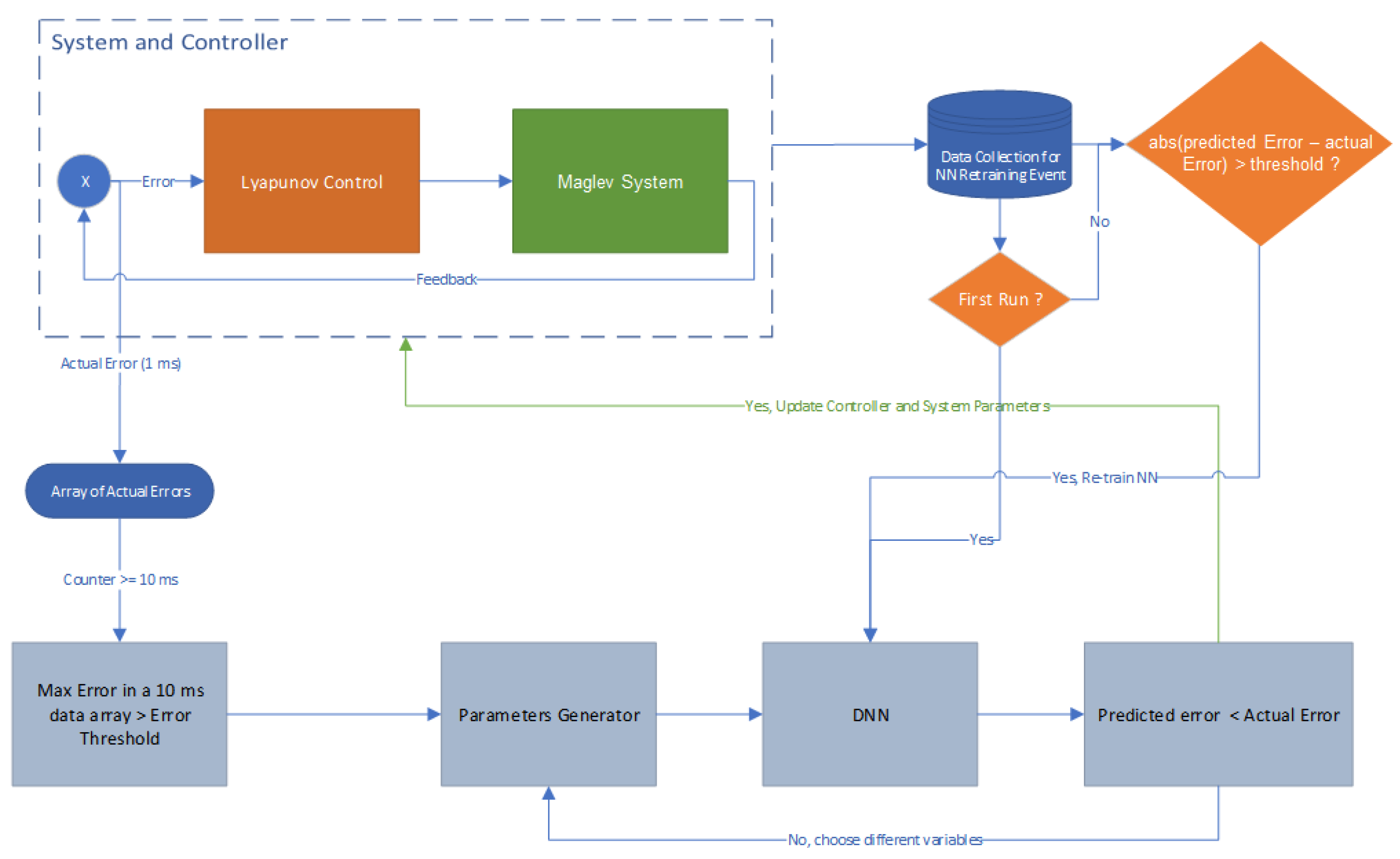
3.2. Network Retraining

It was found that without the use of memory, the retraining phase of the neural network could take longer and, in some situations, continue into an indefinite state without finding the best solution. Because we only examine the change in the average of the system error, the speed with which the system returns to its stable condition has an impact on the retraining phase. The requirement for retraining will not be met if the difference between the prior system error average and the new system error average does not exceed the set point. The network can recall the stable and perturbed history of the system parameters attributable to the new data introduced to the memory. 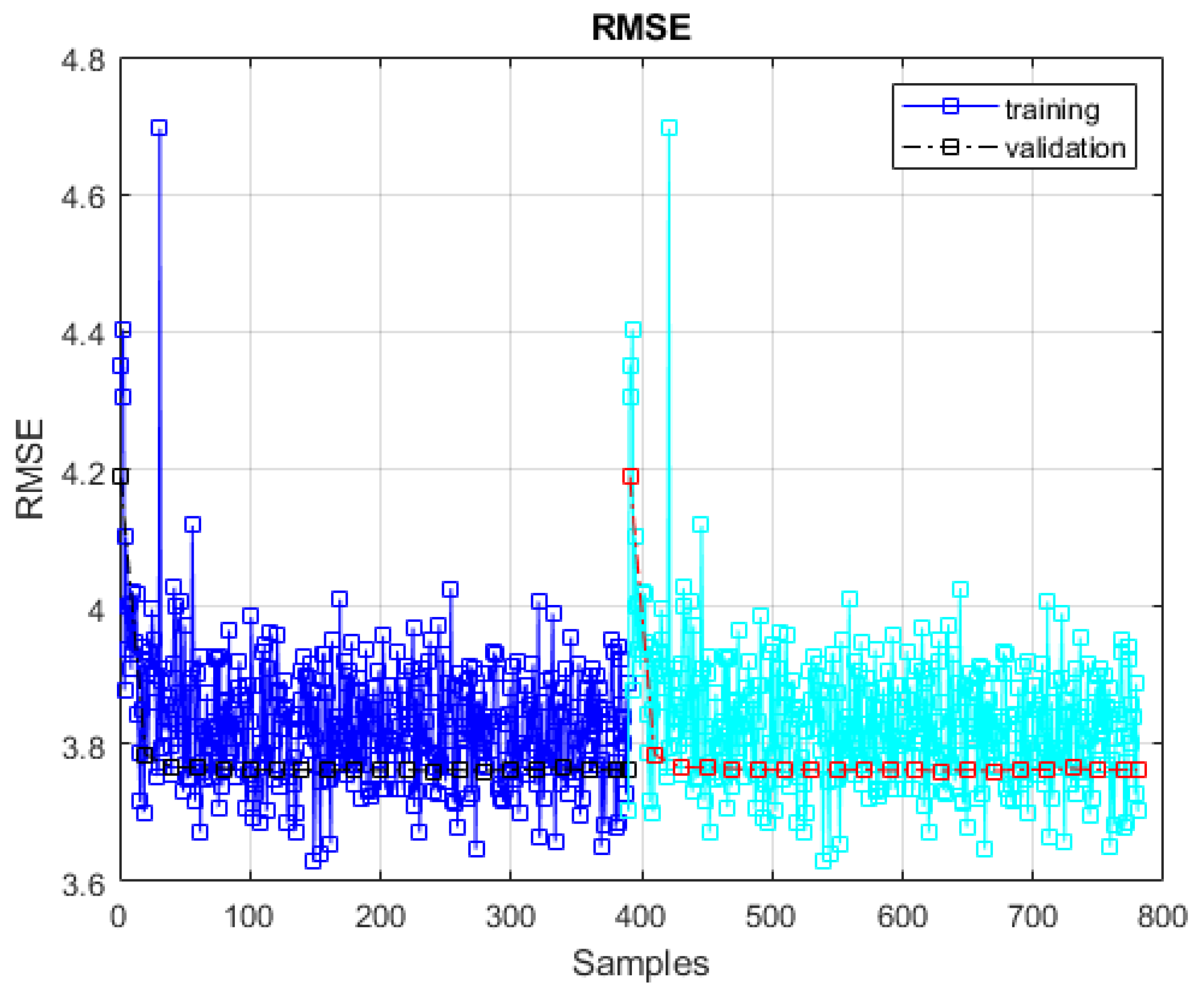Figure 15 presents the flow logic and conditions towards the retraining process. While in Figure 16 the RMSE for training and re-training phase are presented.

4. Conclusions

Dynamic Lyapunov control is applied to a nonlinear Maglev model that is experiencing chaotic behavior. The study shows the effectiveness of dynamic deep learning integration with Lyapunov control allowing an autonomous CPS algorithm where the optimal parameters are found to maintain CPS stability. The algorithm is able to achieve safe parameter recommendations within 0.1 ms to 8 s from triggering the DNN depending on the number of parameters that require change and the type of nonlinear dynamics introduced. The algorithm is shown to yield successful results after testing different scenarios of switching inputs or applying high frequency input. In future studies, unsupervised types of machine learning architectures may be researched. Additionally, another research direction is to enable the deep learning system to select between different types of controllers or strategies based on the type of instability discovered. Adjusting the control mechanism would require additional processing power and data sets, but can be utilized in conjunction with parameter adjustment as a last resort towards system stability. Additionally, sliding mode control can be examined, which, when combined with the deep learning methods utilized in this study, could produce positive outcomes.