A Numerical Multistage Fractured Horizontal Well Model Concerning Hilly-Terrain Well Trajectory in Shale Reservoirs with Natural Fractures

Abstract

Multistage hydraulic fracturing is one of the most prevalent approaches for shale reservoir development. Due to the complexity of constructing reservoir environments for experiments, numerical simulation is a vital method to study flow behavior under reservoir conditions. In this paper, we propose a numerical model that considers a multistage fractured horizontal well with a hilly-terrain trajectory in a shale reservoir with the presence of natural fractures. The model was constructed based on the MATLAB Reservoir Simulation Toolbox and used the Embedded Discrete Fractured Model (EDFM) to describe the interrelationship between the matrix, fractures, and wellbore. The model was then applied to an actual condensate gas well producing from a shale reservoir, and the effects of reservoir parameters on the simulation data were studied based on this well case. The simulation results were highly consistent with the actual production data, which validates the accuracy of this model and proves its potential for predicting future production trends. We extended the discussion to two examples with extreme well trajectories by reviewing the inflow contribution of each hydraulic fracture with respect to fracture pressure, and the changes in static pressure with time. In conclusion, the proposed model is capable of providing simulation results close to reality and thus guiding field design and operation in the fracturing and drilling process.

1. Introduction

Hydraulic fracturing in horizontal wells is a common practice to effectively extract hydrocarbon resources from the formation in industry. This approach can be often seen in the production of hydrocarbon fluids from unconventional reservoirs such as shale, tight formation, and coalbed methane [1]. The relationship between formation pressure and saturation with respect to production time can be analyzed by calculating reservoir productivity based on a fractured horizontal well, thus leading to the law of change in well productivity with time [2]. Given that well productivity is directly related to the total recovered hydrocarbon of a well, a major criterion for economic evaluation, the well productivity is one of the key guiding indexes for the production design and optimization in horizontal well drilling and completion, as well as a major reference to realize the maximum output of oil and gas production.

The calculation of productivity for fractured horizontal wells includes two parts, namely the reservoir and the wellbore. The reservoir part mainly considers characteristics of flow in and between the porous media and fractures [3]. Meanwhile, coupled calculation of matrix and fluid properties and their changes with respect to environmental conditions is performed to obtain the fluid flow distribution within the range of the entire reservoir [4]. The wellbore part focuses on the pipe flow as reservoir fluid migrates to the bottom hole. By calculating the local pressure drop along the wellbore, the relationship between the flowrate of reservoir inflow fluid and wellbore pressure can be obtained [5]. Therefore, an accurate fractured horizontal well productivity calculation requires fine coupling between the reservoir and wellbore.

Currently, existing productivity calculation methods for fractured horizontal wells have established a systematic approach in terms of reservoir simulation, especially for numerical simulation represented by a finite element method and discrete fracture model [6,7]. Notably, the discrete fracture model treats the fracture parameters as one of the boundary conditions of the host reservoir units and thereby reduces the dimension of the fracture lower than the reservoir dimension [8,9]. For example, in a three-dimensional reservoir simulation, fractures are treated as two-dimensional planes existing between reservoir units. In this way, the discrete fracture model significantly improves computational efficiency while ensuring simulation accuracy. Numerical simulation divides the entire reservoir into a finite number of units, couples the flow between fracture and matrix, and solves the governing equation using numerical methods.

In contrast, there have been relatively complete theories and models regarding the pressure distribution and cause of pressure drop in a horizontal wellbore simulation [10]. Models describing the different phases’ distribution and flow regimes have also been pro-posed and testified by experiment. There has been extensive research based on multiphase flow in a hilly-terrain pipe, but most studies were conducted mainly by experimental methods [11]. Due to gravitational effect, under the difference of flowrate between liquid and gas, multiphase mixture in a curved wellbore is likely to form slug flow that introduces instability to the pipeline [12,13]. In actual numerical simulations of reservoir productivity, horizontal wells are often treated as perfectly horizontal and the internal pressure loss is neglected, meaning the wellbore is treated as a source term.

In fact, horizontal wells can exhibit a certain degree of hilly terrain due to factors such as limitation of drilling technology and poor geological conditions. In such cases, the trajectory of the horizontal well is no longer a straight line, but a curve that has an undulating path [14]. Fluid flowing along such a well path can result in an extra pressure drop due to the gravitational effect. When both liquid and gas phases flow within the horizontal well, the liquid is more likely to accumulate at the lower part of the wellbore, thus bringing instability to the wellbore system and a possible decrease in production [15].

Furthermore, when the horizontal well has multiple stages of hydraulic fractures on a curved well path, these hydraulic fractures may locate at different depths along the fractured section. In such a scenario, depth difference leads to pressure difference between each fracture, and thus leads to different amounts of inflow of reservoir fluid to each fracture. This difference results in an uneven contribution of fractures to the overall productivity [16]. Due to the fact that fluid tends to flow from a high to a low pressure zone, the fracture that has a lower pressure may have more reservoir fluid inflow than others [17]. Moreover, if the reservoir pressure is close to the dew point pressure of the reservoir fluid, for instance in a condensate gas reservoir, then phase change involves in the process of reservoir simulation, which poses a significant burden on computation efficiency and accuracy [18,19]. The depth difference between hydraulic fractures at different locations along a hilly-terrain horizontal well becomes a factor that can influence phase change of reservoir fluid when it flows from the reservoir to the fracture, and at last to the wellbore [20]. Thus, it is necessary to study the productivity of a multistage fractured well with a hilly-terrain trajectory, and further quantify the inflow behavior of reservoir fluid when hydraulic fractures are located at different depths [21]. In this case, even though the simplified reservoir–wellbore coupling method (which assumes the horizontal well has a straight trajectory and neglects pressure change within the wellbore) effectively reduces the simulation difficulties and computation burden, a significant error can be introduced in the calculation of productivity [22].

However, despite extensive research focusing on either reservoir simulation or pipe flow simulation, rare studies pivoting on coupling simulation of reservoir and pipe flow concern horizontal wells with hilly-terrain geometry [23,24]. In cases where there is a need to simultaneously consider the reservoir matrix, fractures, and hilly-terrain wellbore, existing numerical simulation methods are insufficient to precisely predict the inflow behavior of each fracture.

To this end, a numerical model considering a hilly-terrain production well trajectory in a shale reservoir was established based on the open-sourced MATLAB Reservoir Simulation Toolbox (MRST). The model simulates the well productivity after multistage hydraulic fracturing. Other than hydraulic fractures, the model considers the presence of natural fractures that intersect with the well and hydraulic fractures. The solving process involves the Peaceman well model [25] and the embedded discrete fracture model (EDFM) [26,27]. The model construction process is illustrated in detail in the following sections.

2. Methodology

2.1. General Procedure

The construction and computation of the model include the following steps.

• Set up the reservoir properties and pressure field and mesh the reservoir into finite units. Define end time and time interval Δt.
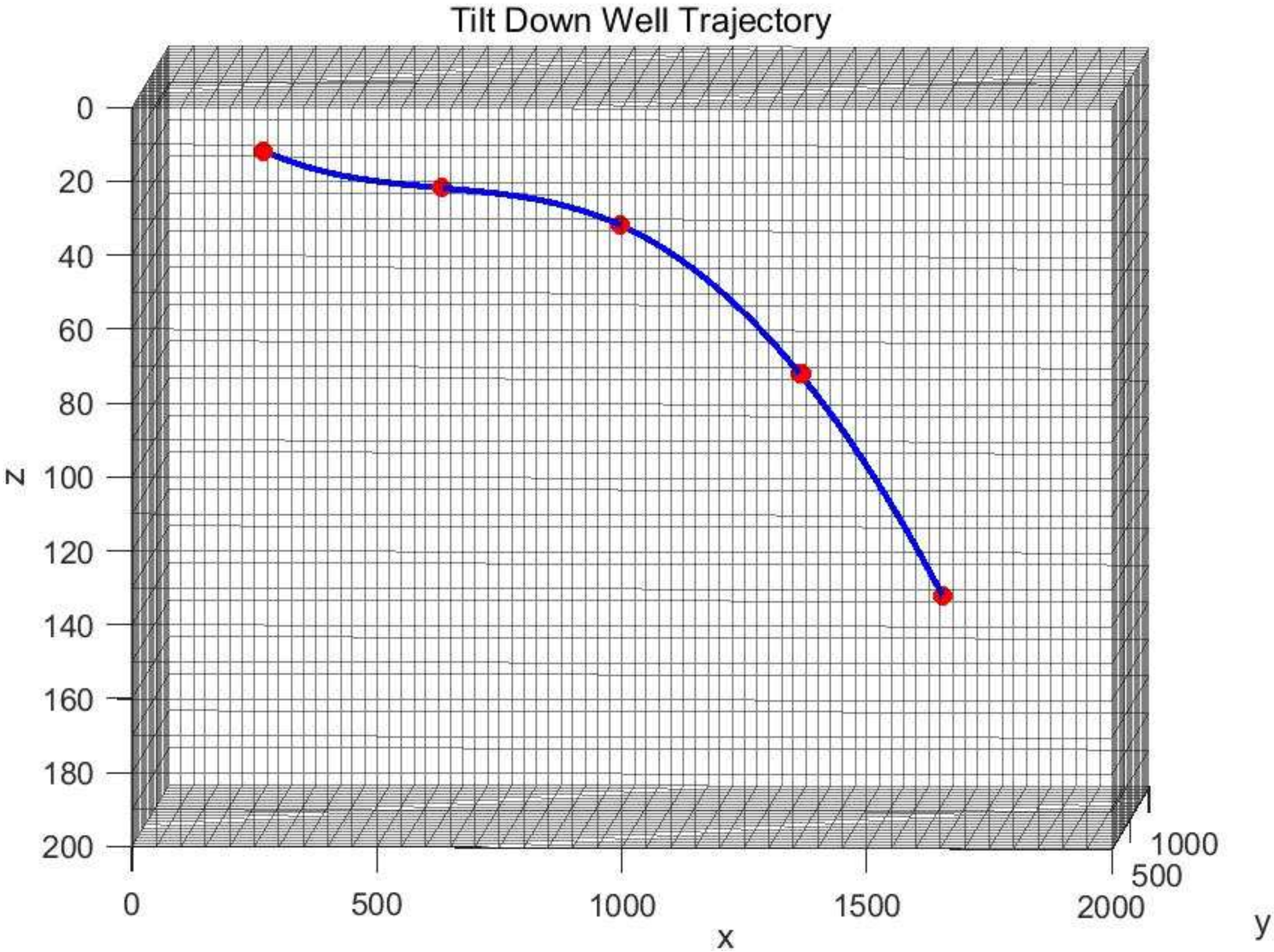
• Pick a number of coordinates of the undulating horizontal well based on model computation efficiency and define well trajectory by using the interpolation method. Similar to the reservoir, the wellbore is divided into wellbore units with wellbore properties defined.
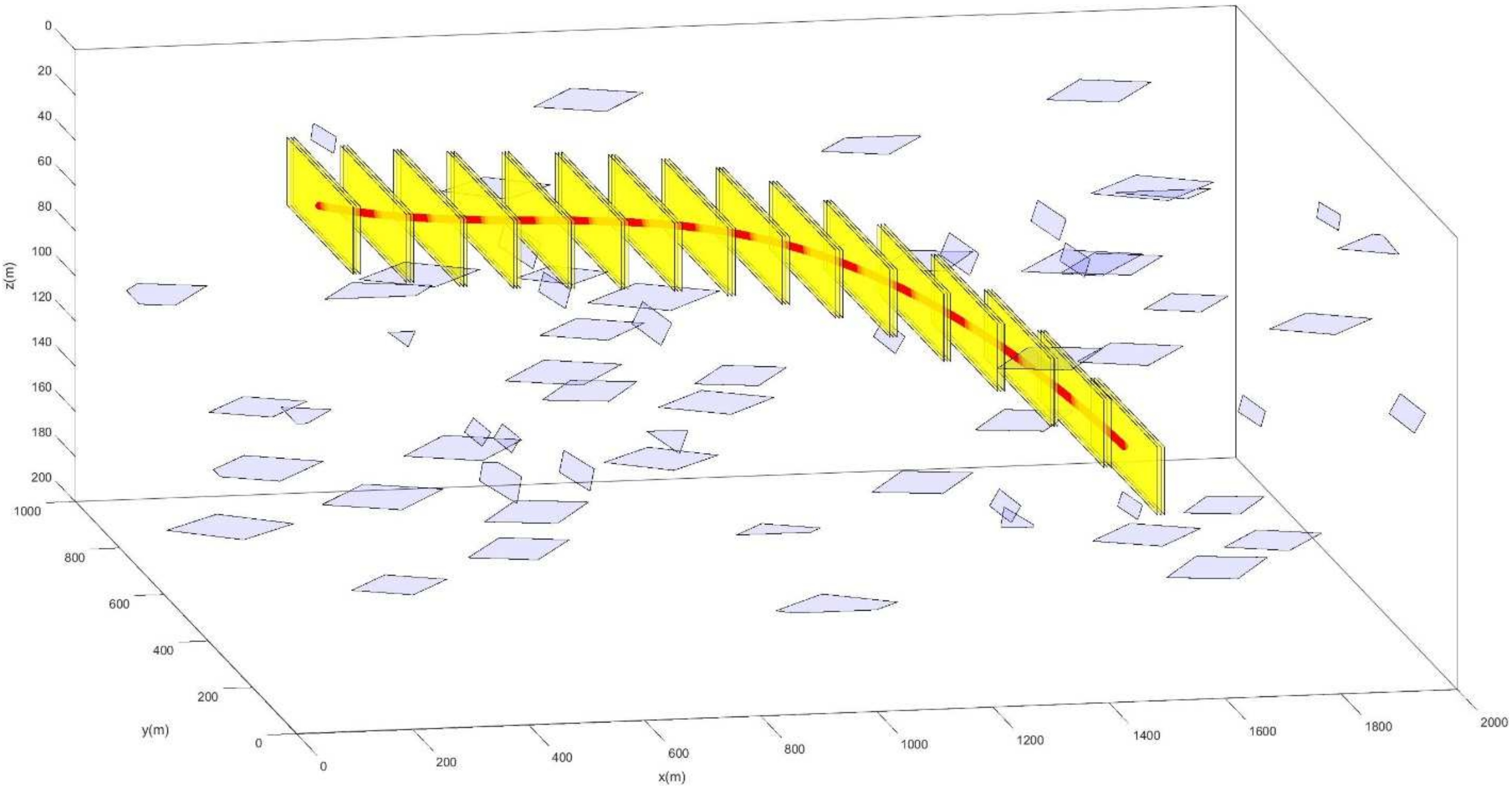
• Define fracture initiation point, fracture boundary, and interval along the well trajectory. Couple the fractures with the matrix unit by using the discrete fracture method and set up fracture properties.
• Couple the flow equations of both reservoir and wellbore from time t to t + Δt. Then, discretize and solve them through the iterative process.
• Calculate the oil and gas flowrate and their corresponding saturations of each reservoir and wellbore unit from time t to t + Δt and obtain well productivity.
• Enter the next time period and repeat steps 4 and 5.

Compared to the conventional model construction procedure, with an extra step of defining separate horizontal well coordinates with an elevation difference, this model is capable of describing the impact of hilly-terrain horizontal wellbore internal pressure changes on productivity at different periods. It can thereby accurately simulate reservoir flow distribution and production at different times.

2.2. Mathematic Model

The building of the mathematical model starts with the setup of initial reservoir properties and the division of reservoir units. Initial reservoir properties include matrix porosity ɸ_m, permeability k_m, initial phase saturation S, and rock compressibility factor. Fluid properties include density ρ_α, viscosity μ_α, relative permeability K_rα of each phase α, dissolved gas–oil ratio R_s, oil–gas ratio R_v, and volumetric factor B_α. Wherein, the relationship between rock compressibility and reservoir pressure is as follows:

$$c_r=\frac{1}{{\varphi }_m}\frac{d{\varphi }_m}{dp}$$

(1)

where c_r is the rock compressibility factor, and p is the reservoir pressure.

To divide the reservoir into units is to divide it into cubes with identical length, height, and width measurements. Other than the geometric partition of reservoir, these cubes are also the units that store the above reservoir properties.

The division of the wellbore is similar to that of the reservoir, in which the wellbore is divided into m segments with each measurement corresponding to the reservoir unit. Likewise, each wellbore unit is more than a geometric partition, but stores parameters such as unit flow length L_w,m, diameter D_w,m, volume V_w,m, depth Z_w,m, wellbore damage s_w,m, and unit centroid location x_w,m.

Different coordinates of the horizontal well are points located on the measured horizontal well trajectory, and can be expressed as:

$$a=x_0,x_1,\dots ,x_i,x_{i+1},\dots ,x_n$$

(2)

where x_o represents the toe-end coordinate while x_n represents the hill-end coordinate of the well. With this notation, the interpolation curve of the horizontal well coordinates can be expressed as follows:

$$[X,Y,Z]=spline(x)$$

(3)

where spline represents cubic spline interpolation.

When constructing a hilly-terrain horizontal well, it is imperative that the fracture centroids locate correctly on the well trajectory. Thus, the coordinates picked to generate well trajectory should contain the points where hydraulic fractures are created. After generating the well trajectory, fracture initiation points are selected to define the hydraulic fracture’s location and geometry. Here they are denoted as [X_i,Y_i,Z_i]. For simplicity, in this model, fractures are treated as upright planes that distribute along the horizontal well. Their four endpoints can be expressed as:

$$\left\{\begin{array}{c}[X_{i1},Y_{i1},Z_{i1}]=[X_i,Y_i-\frac{L_f}{2},Z_i+\frac{H_f}{2}]\\ [X_{i2},Y_{i2},Z_{i2}]=[X_i,Y_i+\frac{L_f}{2},Z_i+\frac{H_f}{2}]\\ [X_{i3},Y_{i3},Z_{i3}]=[X_i,Y_i+\frac{L_f}{2},Z_i-\frac{H_f}{2}]\\ [X_{i4},Y_{i4},Z_{i4}]=[X_i,Y_i-\frac{L_f}{2},Z_i-\frac{H_f}{2}]\end{array}\right.$$

(4)

In this model, for multistage fracturing scenarios, different hydraulic fractures locate and distribute based on fracture interval and facture cluster interval. Each fracture unit stores parameters such as fracture porosity, permeability k_f, length L_f, height H_f, and width W_f.

The generation of fractures in this model selects the embedded discrete fracture method (EDFM) to implicitly describe fractures in reservoir matrix grids, aiming to improve fracture description accuracy and model computation efficiency. An emerging fracture description technique, the EDFM method simplifies fractures to be smooth and parallel planes, and thus obtains the equivalent flow parameters along the fracture’s aperture direction based on the concept of single fracture equivalence and cubic law. This method simplifies fractures by reducing their dimension and thereby significantly improves computation efficiency. Compared with the traditional dual-porosity and permeability model, this model can better simulate the fractures’ geometry form at any angle while ensuring relatively high computation efficiency and accuracy. In this approach, flow is classified in the following 4 ways based on different interunit communication scenarios (intermatrix flow, matrix–fracture flow, intrafracture flow, and interfracture flow. Specifically, flow within fractures that satisfies the Navier-Stokes equation is treated as a source term that satisfies Darcy law, and can be expressed as:

$$q_x^{nnc}={\displaystyle \sum _{m=1}^{N_{nnc}}{A}_m^{nnc}{\displaystyle \sum _{x=1}^{n_p}\frac{k_m^{nnc}{k}_{rx}}{{\mu }_x}}}{\rho }_x[\frac{P_x-{(P_x)}_m^{nnc}}{d_m^{nnc}}]$$

(5)

where N_nnc represents the number of units in non-neighbor connections with a certain matrix unit. The terms A^m_nnc, k^m_nnc, and d^m_nnc represent the area, permeability, and distance of the non-neighbor connection, respectively. These three parameters can be calculated as follows:

$$A^{nnc}=2A_f$$

(6)

$$k^{nnc}=\frac{k_m{k}_f}{k_m+k_f}$$

(7)

$$d^{nnc}=\frac{{\displaystyle {\int }_V{x}_{n}dv}}{V}$$

(8)

The three-phase flow equations consist of the mass balance equation and Darcy equation, and can be expressed as:

$$\begin{array}{l}\frac{\partial }{\partial t}[\varphi ({\rho }_o{S}_o+{\rho }_g{S}_g)]+\nabla ({\rho }_o\stackrel{\rightharpoonup }{v_o}+{\rho }_g\stackrel{\rightharpoonup }{v_g})-({\rho }_o{q}_o+{\rho }_g{q}_g)/V=0\\ \frac{\partial }{\partial t}[\varphi ({\rho }_w{S}_w)]+\nabla ({\rho }_w\stackrel{\rightharpoonup }{v_w})-({\rho }_w{q}_w)/V=0\end{array}$$

(9)

In the equation, the subscripts o, g, and w correspond to the oil, gas, and water phase, respectively. The v term is the flow velocity, q is the source term, and V is the unit volume.

Furthermore, the relationship between velocity and pressure can be represented as:

$$\overrightarrow{v_{\alpha }}=-\frac{K{k}_{r\alpha }}{{\mu }_{\alpha }}\nabla {\mathrm{\Phi }}_{\alpha },\alpha =o,g,w$$

(10)

where subscript α marks phase α.

In each flow unit, there is a constraint condition of saturation, meaning the sum of three-phase saturation equals one.

$$S_g+S_o+S_w=1$$

(11)

Within the wellbore, the three-phase flow equations can be expressed by mass balance equations and the pipe flow velocity–pressure equation. Here, the mass balance equations are as follows:

$$\begin{array}{l}{\partial }_t(b_w{y}_w)+{\partial }_x(b_w{y}_w)-b_w{q}_w=0\\ {\partial }_t(b_o{y}_o+b_g{R}_v{y}_g)+{\partial }_x(b_o{v}_o+b_g{R}_v{v}_g)-b_o{q}_o-b_g{R}_v{q}_g=0\\ {\partial }_t(b_g{y}_g+b_{\mathrm{o}}{R}_s{y}_o)+{\partial }_x(b_g{v}_g+b_o{R}_s{v}_o)-b_g{q}_g-b_o{R}_s{q}_o=0\end{array}$$

(12)

where the coupling term q_α is the phase flow rate that flows in or out of the wellbore unit, and can be written as:

$$q_{\alpha }=WI\frac{K{K}_{r\alpha }{\rho }_{\alpha }}{{\mu }_{\alpha }{B}_{\alpha }}[P_{bh}-P_{\alpha }-{\rho }_{\alpha }g(Z_m-Z)]{\delta }_m,\alpha =o,g,s$$

(13)

In this equation, δ is the Dirac function defined in the centroid of the wellbore flow unit, P_bh is the flow unit’s pressure, WI is the wellbore index of the corresponding wellbore flow unit, and Z is the depth of the corresponding matrix unit.

The pipe flow velocity–pressure equation can be expressed as:

$$\nabla p-g\rho \nabla Z_w-\frac{\rho u_c{}^2}{2C_v{}^2}+\frac{2f{L}_w}{D_w}\rho u^2=0$$

(14)

In this equation, g is the gravitational acceleration, u_c and u represent the flow velocity in the choke and horizontal well, respectively, C_v is the flow coefficient of choke, and f represents the frictional factor. All fluid parameters in this formula are physical parameters of oil–gas–water mixture fluid.

The above Equations (5)–(14) will were discretized using the MATLAB Reservoir Simulation Toolbox (MRST) for the sequential implicit coupling framework. At the beginning of the calculation, reservoir boundary conditions can be set as closed or constant pressure boundary. The initial condition refers to the pressure at corresponding reservoir depth with or without the consideration of gravity. The discrete phase velocity of the equation (oil phase as an example) is expressed by a two-point flux approximation scheme (TPFA):

$$\stackrel{\rightharpoonup }{v_o}=-T_{ik}{\lambda }_o^{n+1}grad(P_o^{n+1})$$

(15)

Once the above equation is discretized, it can be expressed by the Newton–Raphson iteration method:

$$\frac{\partial R^{k+1}}{\partial X}\Delta X=-R^{k+1}$$

(16)

where the term on the left-hand side of the equation is the Jacobian matrix, and X is the initial variable.

Once each time step is calculated, reservoir pressure and saturation distribution are updated, thus making well productivity available.

This model is constructed based on the reservoir matrix and fracture meshing tool of the MATLAB Reservoir Simulation Toolbox (MRST), which will be introduced specifically in the following section. This study conducts a numerical simulation of fractured hilly-terrain horizontal well on productivity and analyzes the productivity of a multi-stage fractured horizontal well under the influence of hilly-terrain well trajectory. A hybrid numerical simulation program based on structured grids, discrete fracture, and a discrete well was developed for horizontal wells with undulating trajectory, where hydraulic fractures and the wellbore were treated implicitly. The program simultaneously considers trans-scale flow of multiphase (oil-gas-water) flow in reservoir matrix, fracture, and wellbore, calculates the characteristics of change in reservoir pressure and saturation in terms of space and time, and obtains the corresponding productivity of the well to analyze the impact caused by hilly-terrain horizontal well trajectory.

3. Modeling

This model was built using the MATLAB Reservoir Simulation Toolbox (MRST), an open-sourced toolbox based on MATLAB for reservoir modeling and simulation [28]. The main structure of the module is divided into the minimum core module, providing basic data structure and function, and a large number of additional modules, providing discretization, solver, physical model, various simulators, and workflow tools [29].

Reservoir numerical simulation based on MRST starts with the introduction of data objects to track all the different entities that make up these objects. These data objects include:

• State structure: unknown pressure, saturation, concentration, fluxes between units, and unknowns related to wells;
• Grid structure: geometry and topological structure of meshes;
• Rock structure: rock physical data such as porosity, permeability, and net to gross ratio;
• Transmissibility matrix: flow multiplier between neighboring units;
• Fluid structure: a set of function handles that can calculate fluid density and viscosity and further evaluate parameters such as relative permeability and formation volume factor;
• Additional structure: additional conditions including driving mechanism, source conditions, and boundary conditions;
• Optional operator structure that contains discrete operators for differentiation and averaging.

In the process, these data objects are passed as parameters to the solver or function to perform subtasks such as calculation of subsequent equations. The overall structure of this model consists of 5 modules, which are as follows:

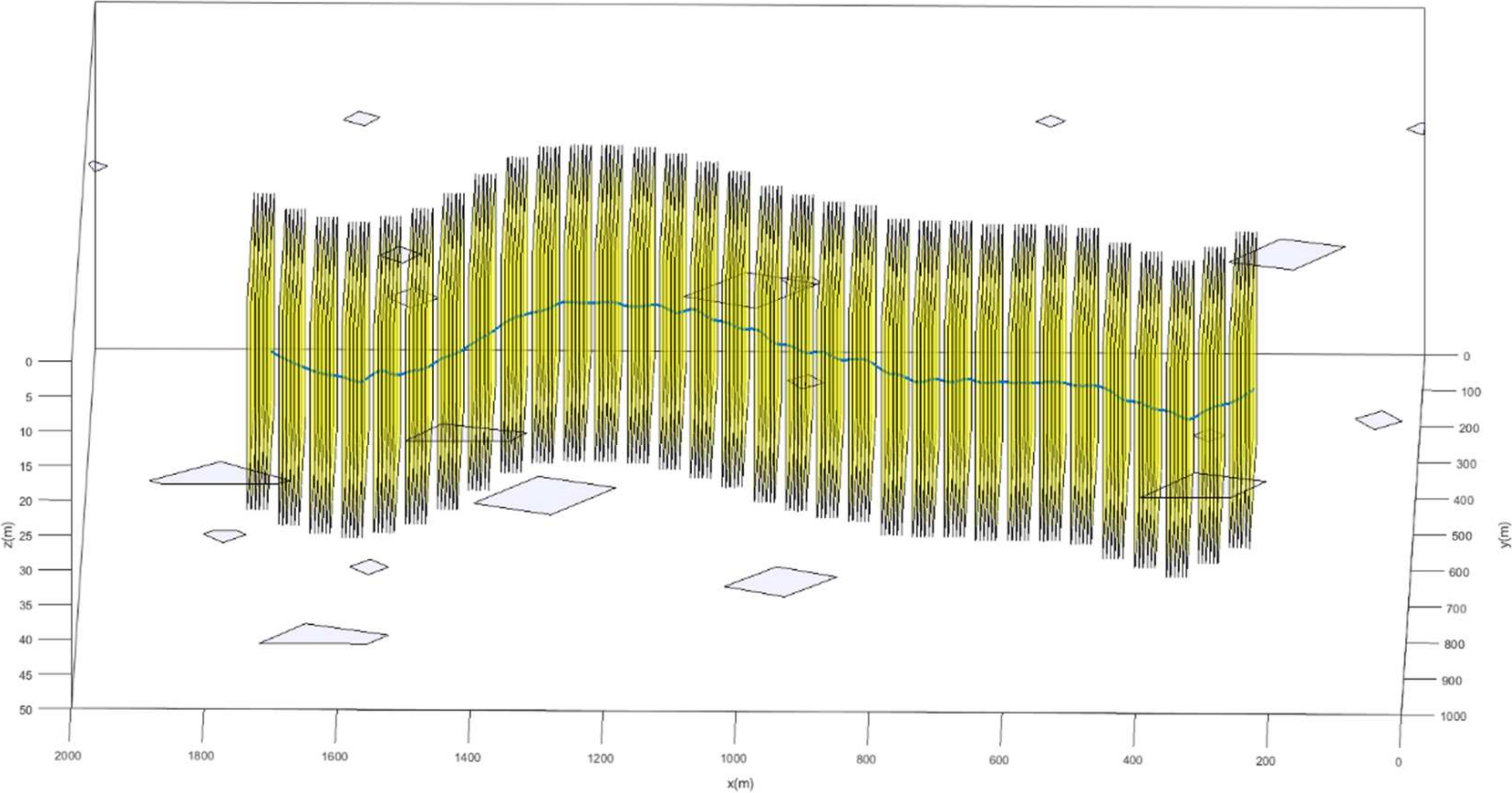
• Geometric and meshing module: establishes reservoir structured matrix grids according to the actual geological structure and determine the locations of the corresponding well and hydraulic fracture location, so as to implicitly characterize fractures, divide the wellbore based on matrix grids, and thereby form complete reservoir flow units;
• Parameter acquisition and assignment module: acquires physical parameters of the reservoir, hydraulic fractures, and well, and assigns values to reservoir flow units;
• Physical model module: plugs the parameters collected by the previous module into fluid flow equations, and forms discrete equations based on flow units, namely the nonlinear calculation matrix;
• Computation module: solves the nonlinear calculation matrix in the previous module by using the Newton–Raphson method to obtain a converged solution of pressure and saturation;
• Prediction module: obtains, analyzes, and optimizes the well production according to the previously given solutions at each time period.

4. Validation

4.1. Validation of Model Accuracy

This model was modified and applied to calculate the well productivity of a multi-stage fractured horizontal well in a condensate gas reservoir. Simulating production from a condensate reservoir can be challenging, as retrograde condensation occurs during the migration of fluid from the reservoir to the wellbore. Phase changes and the interaction between oil and gas phases in the reservoir bring nonlinear characteristics to the simulation, which can largely lower the possibility of a converged result. Existing studies have simulated condensate reservoirs using a modified black oil model or compositional model [30,31]. Together with a hilly-terrain well trajectory, the small pressure difference between formation pressure and fluid dew point results in a retrograde problem that hinders the production.

Indeed, there are many commercial software programs capable of simulating reservoirs and coupling with well calculations. Different from this software, the MRST, as an open-sourced toolbox, allows users to perform secondary programing to adjust and modify the simulation process based on their own research purposes.

In this study, to reduce the computational burden while ensuring accuracy to the greatest extent, this model uses a pre-imported fluid property file to better describe the phase behavior of condensate gas. The horizontal well trajectory of the case well is shown in Figure 1.

In Figure 1, the trajectory is generated by 64 coordinates in total to construct a horizontal well section 1500 m in length. The red dots represent these coordinates, and the blue line represents the well trajectory generated by interpolation. Multistage fracturing was conducted with 32 stages from toe- to heel-end, which is illustrated in Figure 2.

In Figure 2, the model of the case horizontal well with hydraulic and natural fractures is shown. Each yellow rectangle represents one hydraulic fracture. In this model, for the sake of efficiency, all hydraulic fractures were assumed to have identical geometry and distributed with equal interval distance along the trajectory. The uneven quadrangles are stochastic natural fractures generated based on a micro-seismic report of the target reservoir.

The output of this model mainly includes the static pressure, three-phase production, and the three phases’ saturations changing with respect to time. Herein, the oil and gas production of this model were compared with actual production data to validate the accuracy of this model. The output was exported from the simulation results and plotted together with the actual production data since the production began, which are shown in Figure 3 and Figure 4.

In Figure 3 and Figure 4, except for a few abnormal points on the actual production data, both oil and gas production are consistent with the actual production data. This consistency sufficiently validates the accuracy of the model and has proved that the model is capable of exhibiting future production trends.

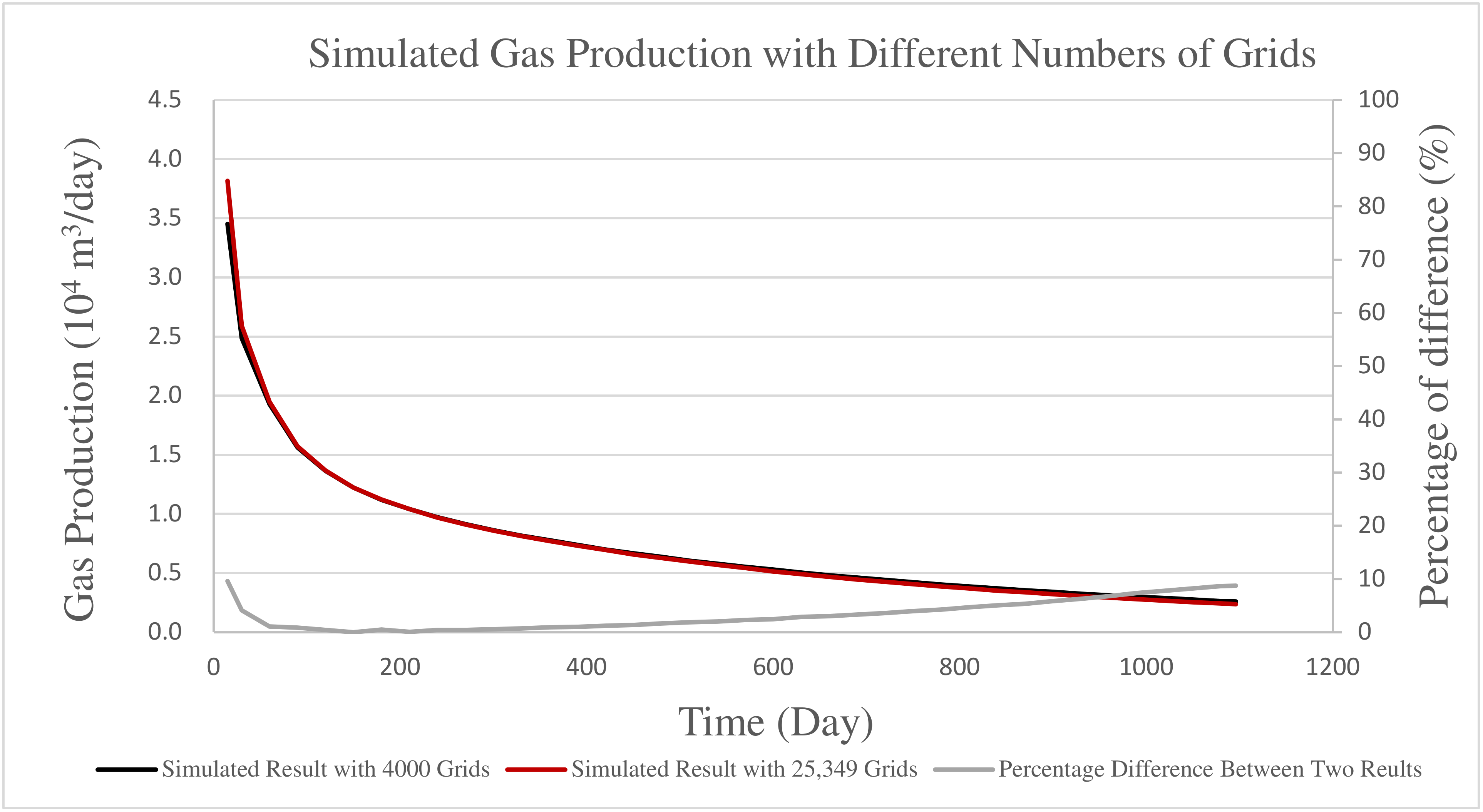
4.2. Validation of Grid Independence

The reservoir in this study was set to 2000 m in length, 1000 m in width, and 50 m in height. The grid size was initially set to 50 m in length, 50 m in width, and 10 m in height. The number of grids was 4000. To validate the grid independence and further examine the accuracy of this model, the grid size was then adjusted to 25 m in length, 25 m in width, and 10 m in height. The number of grids then became 25,349. While parameters other than the grid size were kept unchanged, the simulation was conducted again. Since the case well was drilled to a condensate gas reservoir and mostly produced gas, the comparison was made primarily on gas production.

As shown in Figure 5, the red and black lines are the two sets of simulated gas production data that correspond to the values in the y-axis to the left, while the gray line represents the difference of the two sets of data divided by the production simulated by using 25,349 grids. The result produced by the simulation with smaller grid size is lower than that produced by the one with larger grid size, and thus more accurately describes production in real case. Overall, the results produced by two cases with different grid sizes are consistent, with a percentage of difference less than 10 percent, proving the grid independency of the proposed model.

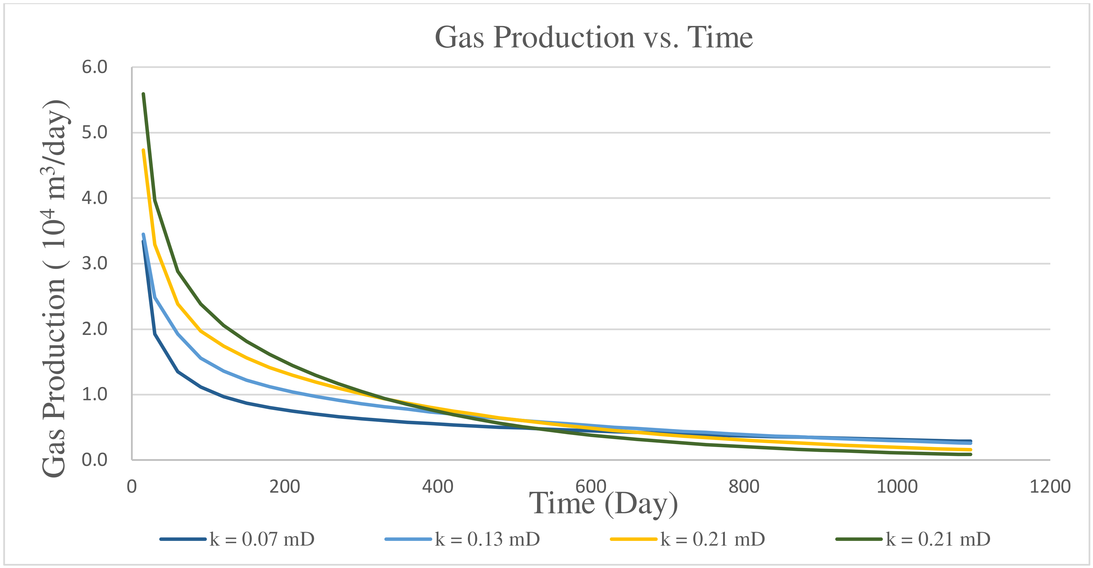
4.3. Effect of Formation Parameters on Simulated Results

With other parameters unchanged, the formation permeability was set to 0.07 mD, 0.21 mD, and 0.3 mD, respectively, in addition to original value of 0.13 mD. The simulated gas productions were then plotted on Figure 6.

As shown in Figure 6, higher permeability leads to higher production at the beginning of production and a faster production decline at the later stage. Therefore, the curve representing the formation with a permeability of 0.3 mD has the highest production at first and has the lowest production at the production end, whereas the 0.07 mD curve has the lowest production at first and the highest production in the long term. This phenomenon exemplifies the fact that fluids in formation with higher permeability can be produced faster than those in formation with lower permeability; however, this comes with the cost of faster reservoir pressure decline leading to a relatively low production rate in the long term.

In addition to permeability, formation porosity can be a key factor that affects the well’s productivity. With other parameters unchanged, the formation average porosity was set to 0.0131, 0.0262, and 0.0786, respectively, in addition to the original value of 0.0524. The simulated gas productions were then plotted in Figure 7.

In contrast to that of changing permeability, the effect of changing porosity on simulated gas production is rather significant. The curve that represents the porosity of 0.0131 approximately halves the 0.0786 porosity curve, and there is no intersection on the four curves plotted above. This means the formation porosity can affect the total production considerably, as a less porous formation hinders the flow within it.

The number of natural fractures in the target formation can also be a factor that influences well productivity. According to the micro-seismic test result, except for a few detected at the midway of the hydraulic fracturing section, natural fractures were not generally developed in the formation of the case well. Therefore, this simulation originally was set to generate 20 natural fractures distributed in the formation matrix. With other parameters unchanged, the simulation was then set to generate 30, 60, and 200 natural fractures, respectively, in addition to the original value of 20. The simulated gas productions were plotted in Figure 8.

As shown in Figure 8, the simulated gas productions at different natural fracture amounts overlap with each other except for at the beginning of production, where a noticeable difference can be observed. This phenomenon indicates that the number of fractures has a small effect on the overall production of the case well, as the fracture permeability of the fractures in the four curves remained unchanged.

Furthermore, to compare and see the simulation difference between a multisegment well with a hilly-terrain trajectory and a conventional well with a straight trajectory, the simulation was conducted under the same conditions but with a straight trajectory.

The hilly-terrain case well trajectory was generated by the micro-seismic report of the actual production well, with a length of 1500 m and a depth difference less than 20 m. The comparison case eliminates the 20 m depth difference and assumes the well trajectory is perfectly horizontal and straight. The simulated production data were then plotted in Figure 9 to observe the difference between the two well calculation methods.

As shown in Figure 9, the simulation using a hilly-terrain well trajectory was generally consistent with but slightly lower than the simulation using a straight well trajectory. As the hilly-terrain well trajectory case involved pressure changes caused by gravitational and frictional effects within the wellbore, the simulated production was lower than the straight well trajectory case. Even though the percentage difference is generally less than 10% despite some turbulence at the starting point, it is worth noting that this difference was found in the case of a depth difference less than 20 m in a 1500 m long horizontal well. In a case in which the well has a depth difference higher than 20 m, even over 100 m, in the same well length, the difference can be significant and the influence brought by a hilly-terrain well trajectory on well productivity cannot be ignored.

5. Discussion

To further explore the impact of undulating well trajectory on a well’s productivity, two examples consider more extreme well trajectories where depth displacement can reach over 100 m in a 1.5 km horizontal well section. The first example is shown in Figure 10 and has a tilt-up trajectory. Figure 11 shows the distribution and density of hydraulic fractures along the well, which are divided into 16 stages with two fractures at each stage. Figure 11 also shows the locations of natural fractures, and some of them are observed to be intersecting with hydraulic fractures and the wellbore. The second example, also shown in Figure 12 and Figure 13, demonstrates a well with tilt-down trajectory.

As mentioned previously, in this study, we aimed to create a coupled simulation of the reservoir with natural fractures and a hilly-terrain horizontal well; thus, it was vital to specifically observe the uneven inflow behavior of hydraulic fractures. For the two cases generated above, the flowrate at each hydraulic fracture was pulled out and plotted together with the fracture pressure, as shown in Figure 14 and Figure 15. The x-axis at both figures represents the first hydraulic fracture at the heel-end of the well to the very last hydraulic fracture at the toe-end. The production contribution of each fracture was calculated by the flowrate at each hydraulic fracture divided by the total flowrate at reservoir conditions.

In Figure 14 and Figure 15, a similar relationship between fracture pressure and production contribution can be observed. Higher fracture pressure results in a lower flowrate from reservoir to fracture, whereas lower pressure brings a higher flowrate from the reservoir. Specifically, in the tilt-up case, the hydraulic fracture at the toe-end contributes to almost 3.5% of the total production, which is over eight times the fracture at the heel end, because of the lower pressure at a shallower depth.

Herein, the production of oil and gas with respect to time was exported, together with static pressure distribution at different production times. The simulated production data of the tilt-up well case are shown in Figure 16, and the static pressure distribution at different times in this case is shown in Figure 17.

The simulated production data of the tilt-down well case are shown in Figure 18, and the static pressure distribution at different times in this case is shown in Figure 19.

The two well cases had identical reservoir and wellbore parameters except for their different well trajectories. The difference in depth of these two cases is the same, but the two trajectories have different directions of curvature. In Figure 17 and Figure 19, the pressure distribution of both well cases are similar and show rapid pressure decline at the heel-end of the wellbore regardless of the curved directions. According to the simulated production data of the two well cases in Figure 16 and Figure 18, both wells exhibit a similar production trend, and the production shows a small difference in values. However, by overlaying the production datasets of the two well cases, shown in Figure 20, we can see that the tilt-up case has higher oil and gas production, which is attributed to lower toe-end pressure of the well due to gravitational effects.

6. Summary

In this study, a numerical simulation model that considers hilly-terrain well trajectory in the presence of natural fractures and hydraulic fractures is proposed. The model simulates the well’s productivity by dividing the reservoir into structured grids and using the embedded discrete fracture model to describe flow behavior between different grids. Several conclusions are drawn, as follows:

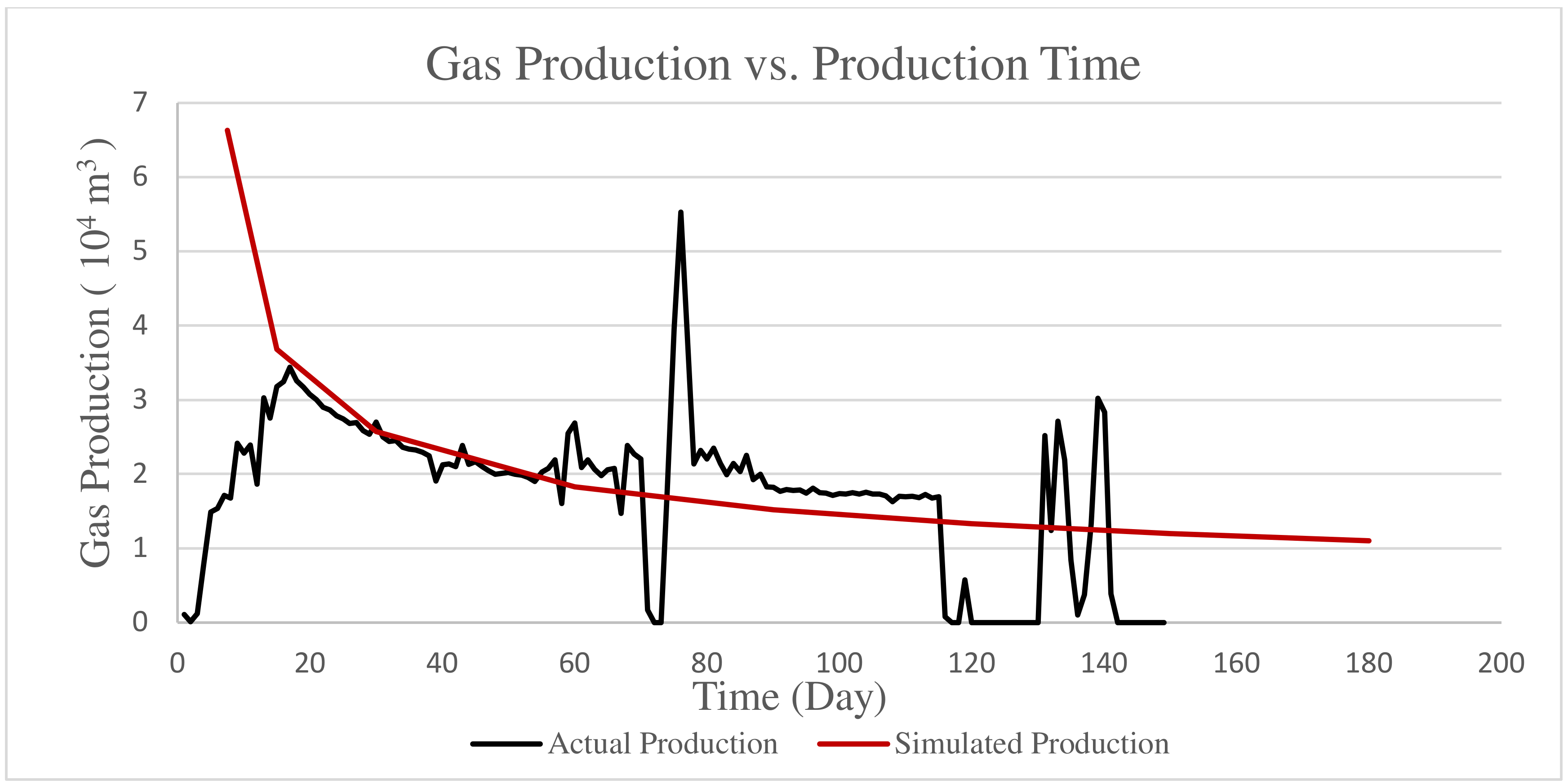
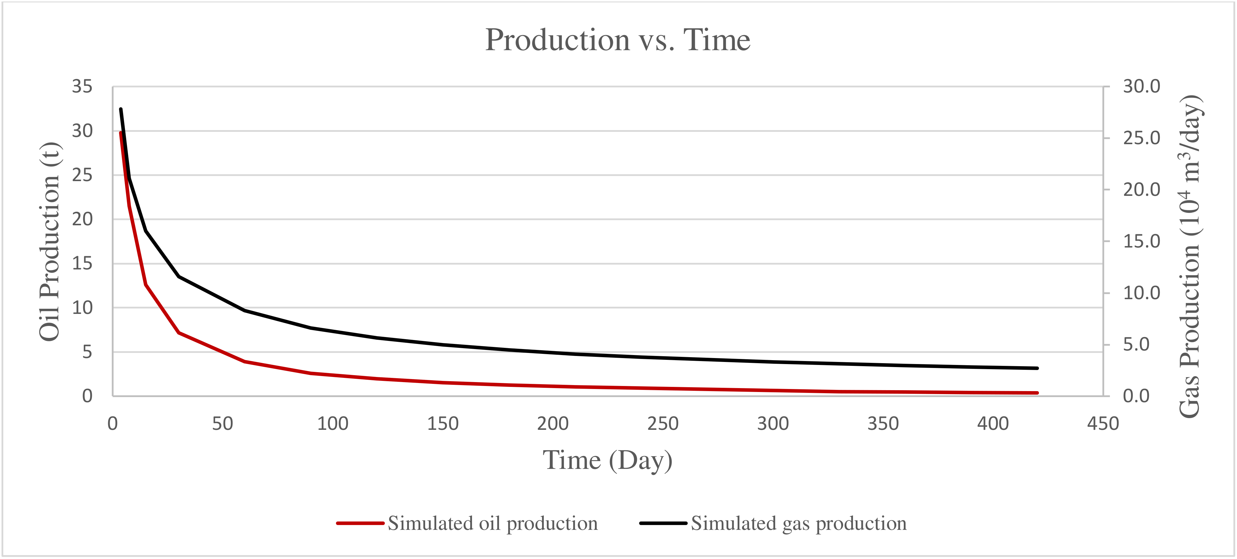
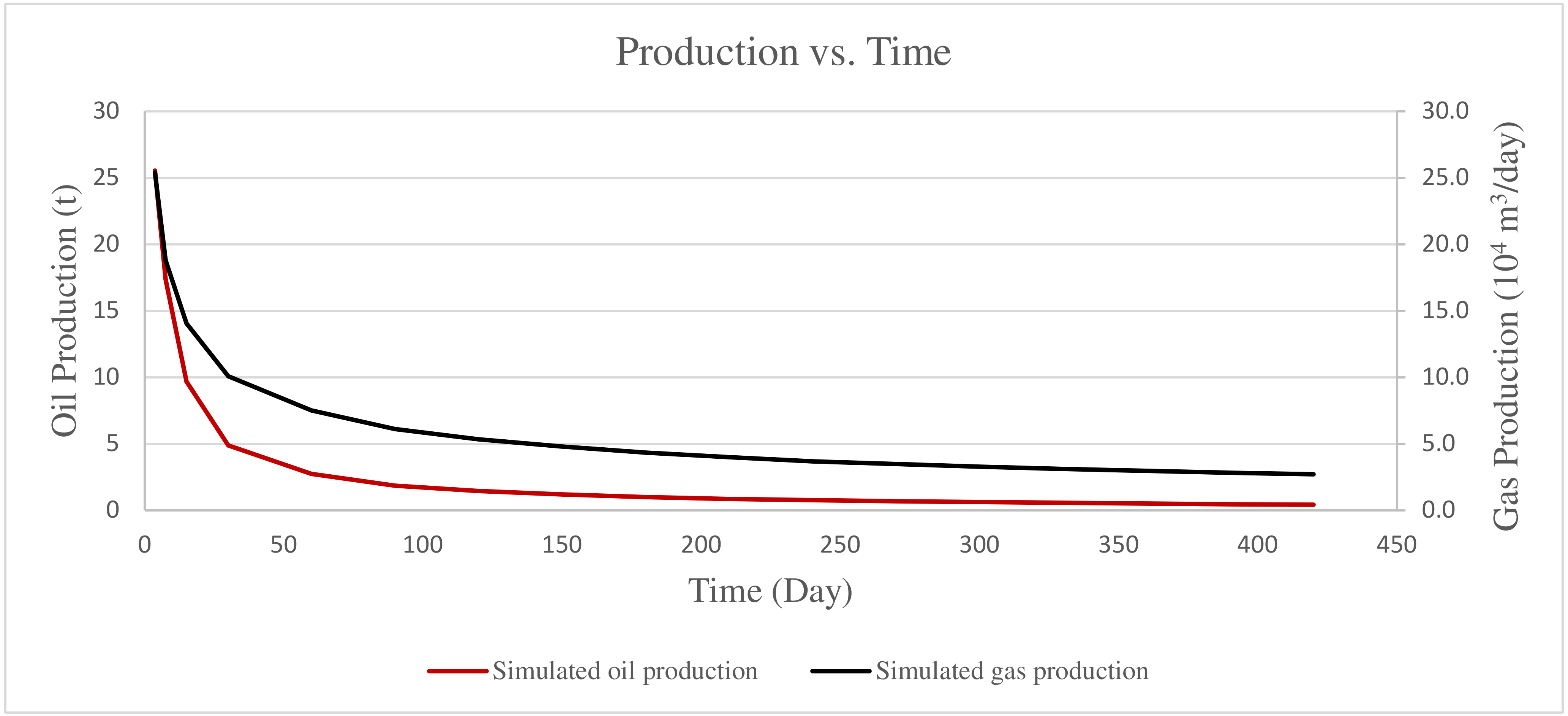
• The simulation results of the case well are compared to the actual production data. The high consistency between the two datasets has proved the accuracy of this model and its capability of predicting a well’s future production trend.
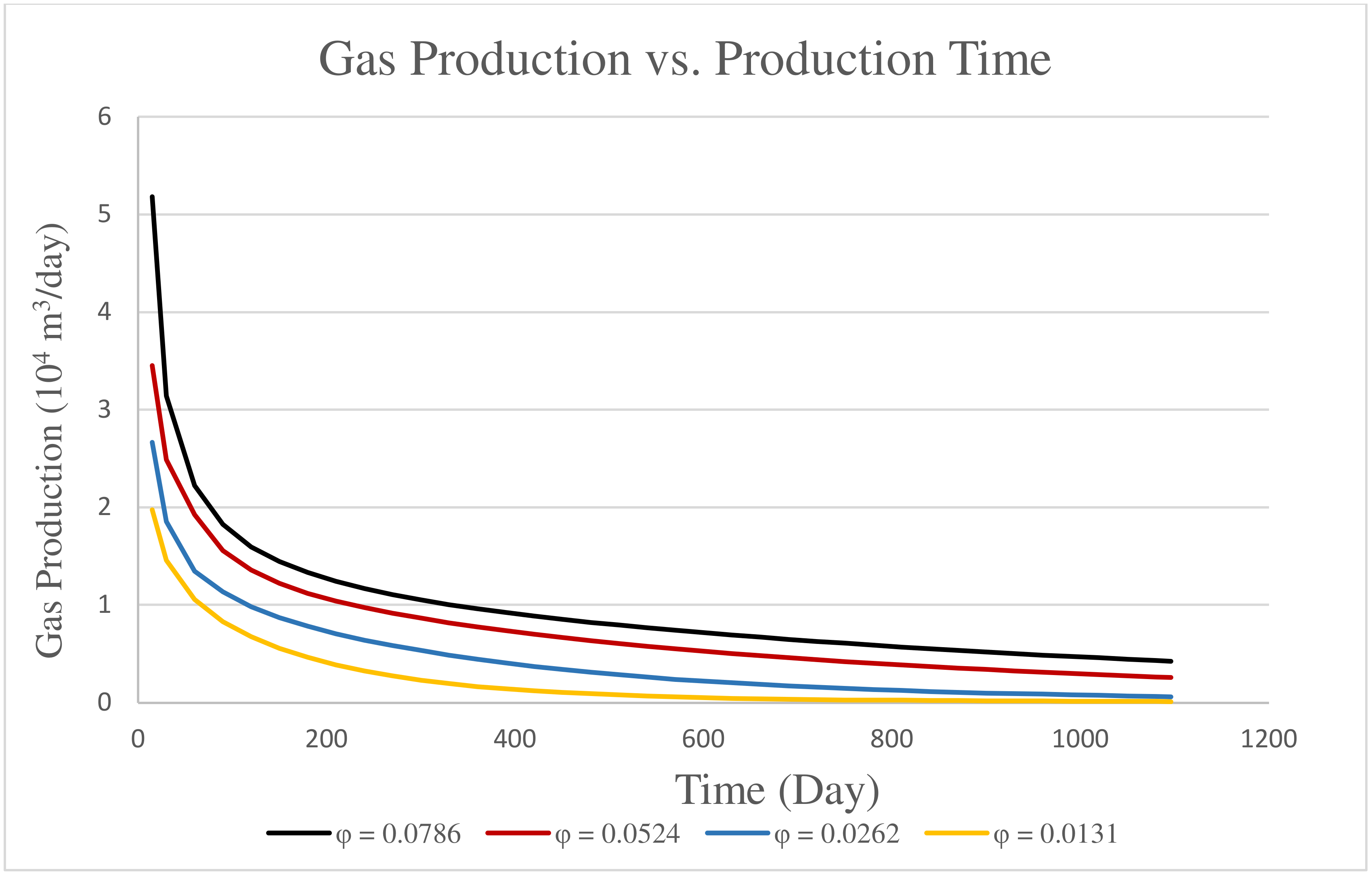
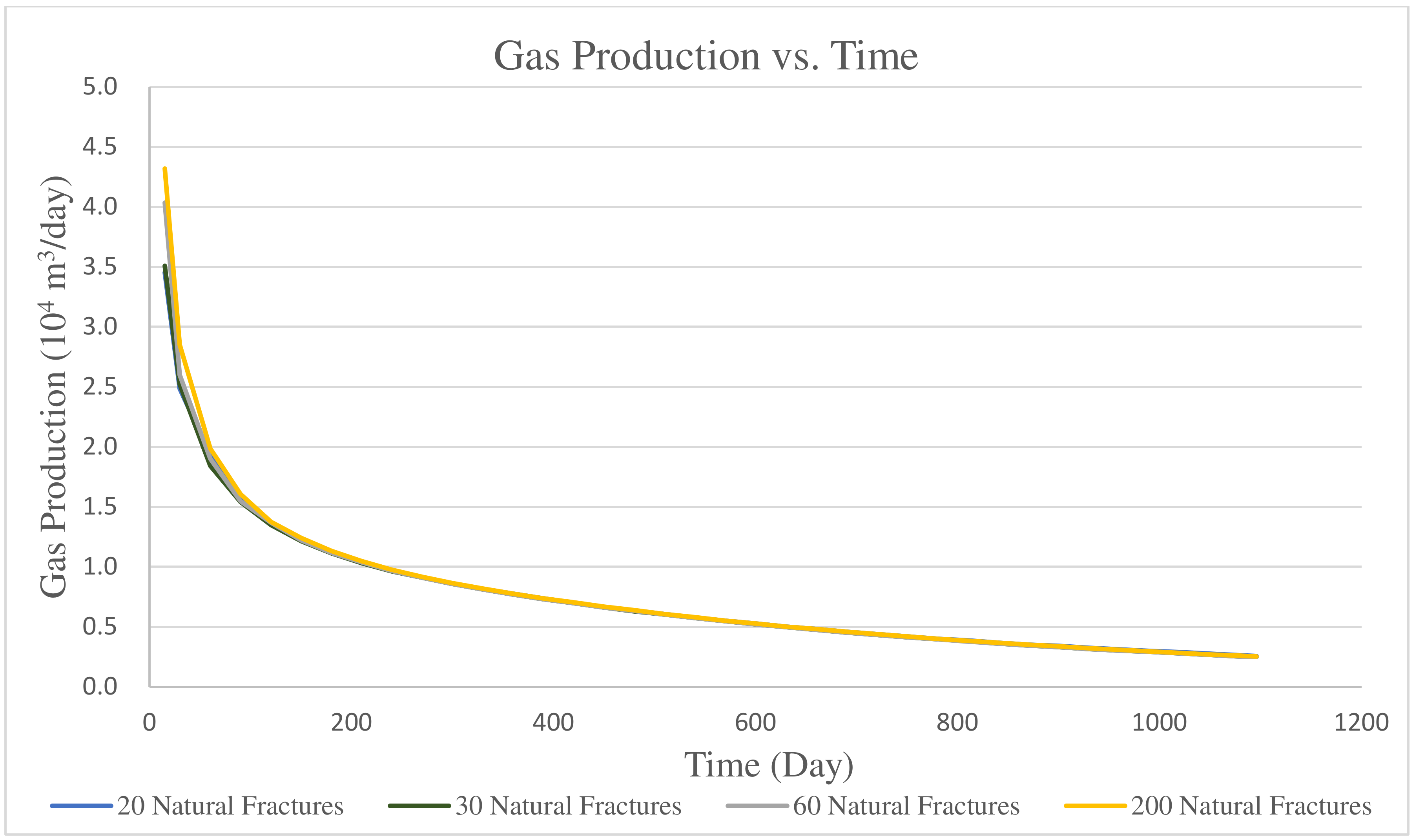
• The effect of reservoir parameters on simulated results was studied, and by keeping other parameters unchanged, the effect of changes in reservoir permeability, porosity, and the number of natural fractures was analyzed. The reservoir porosity had the most significant impact on the overall productivity of the well, followed by permeability and the number of natural fractures.
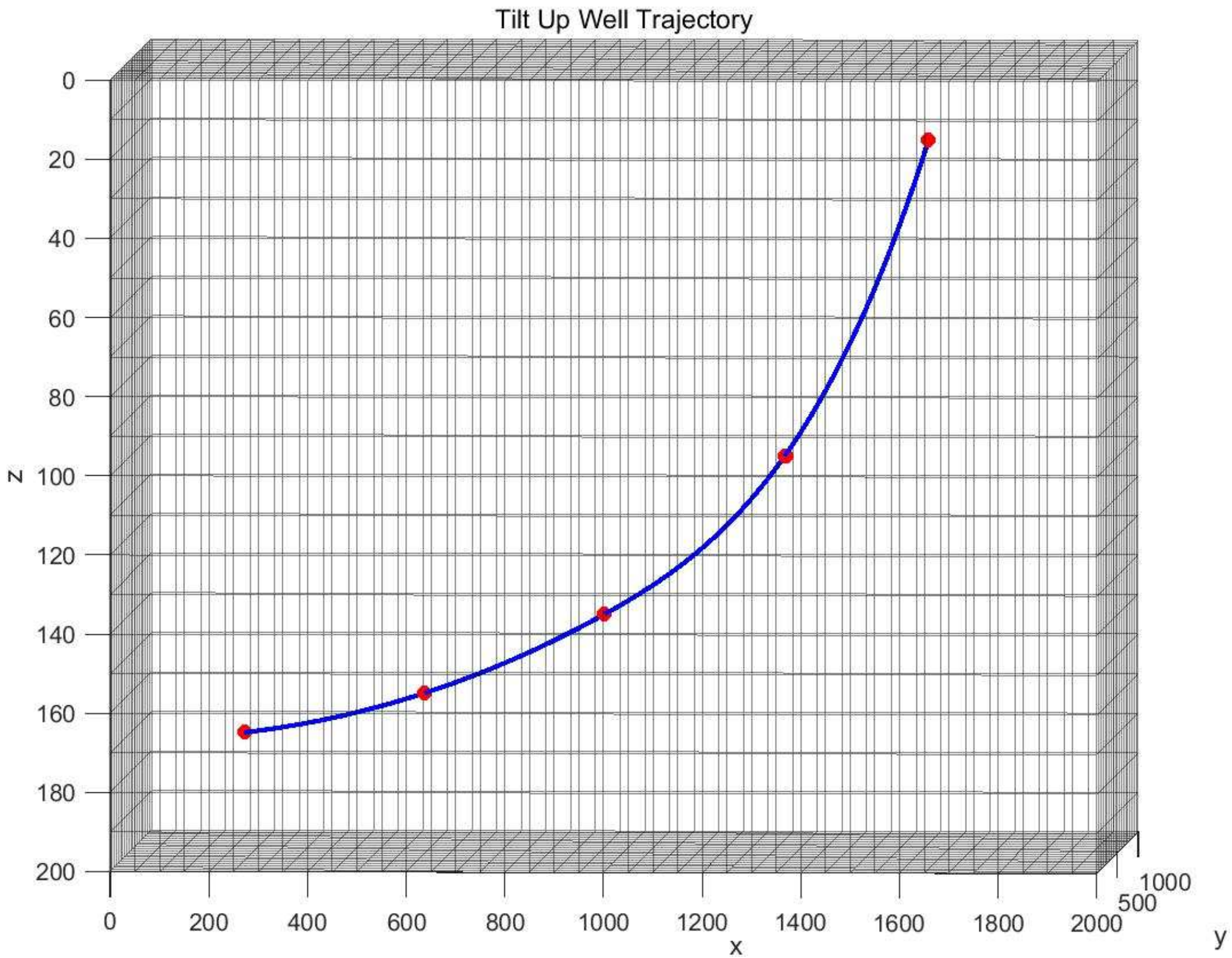
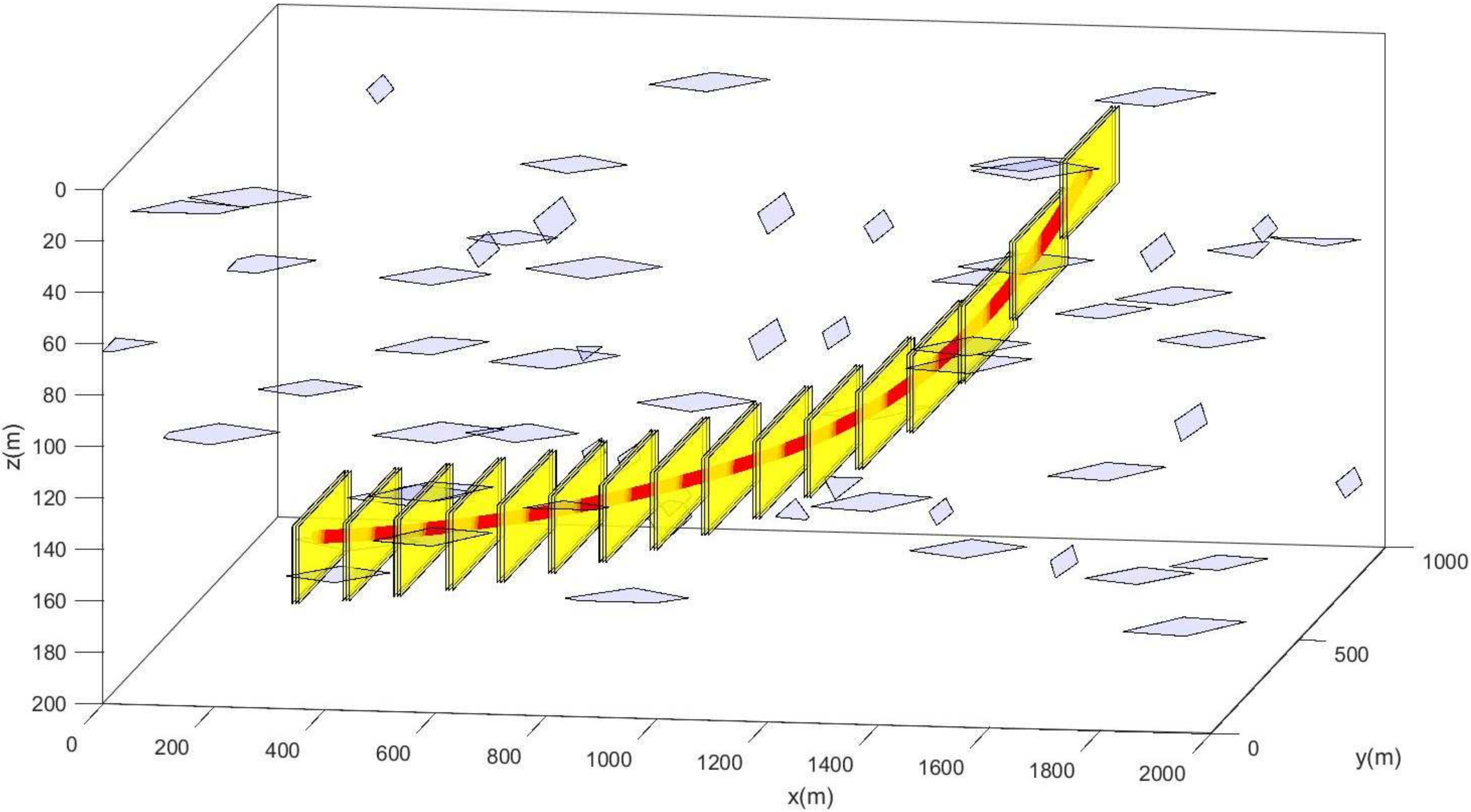
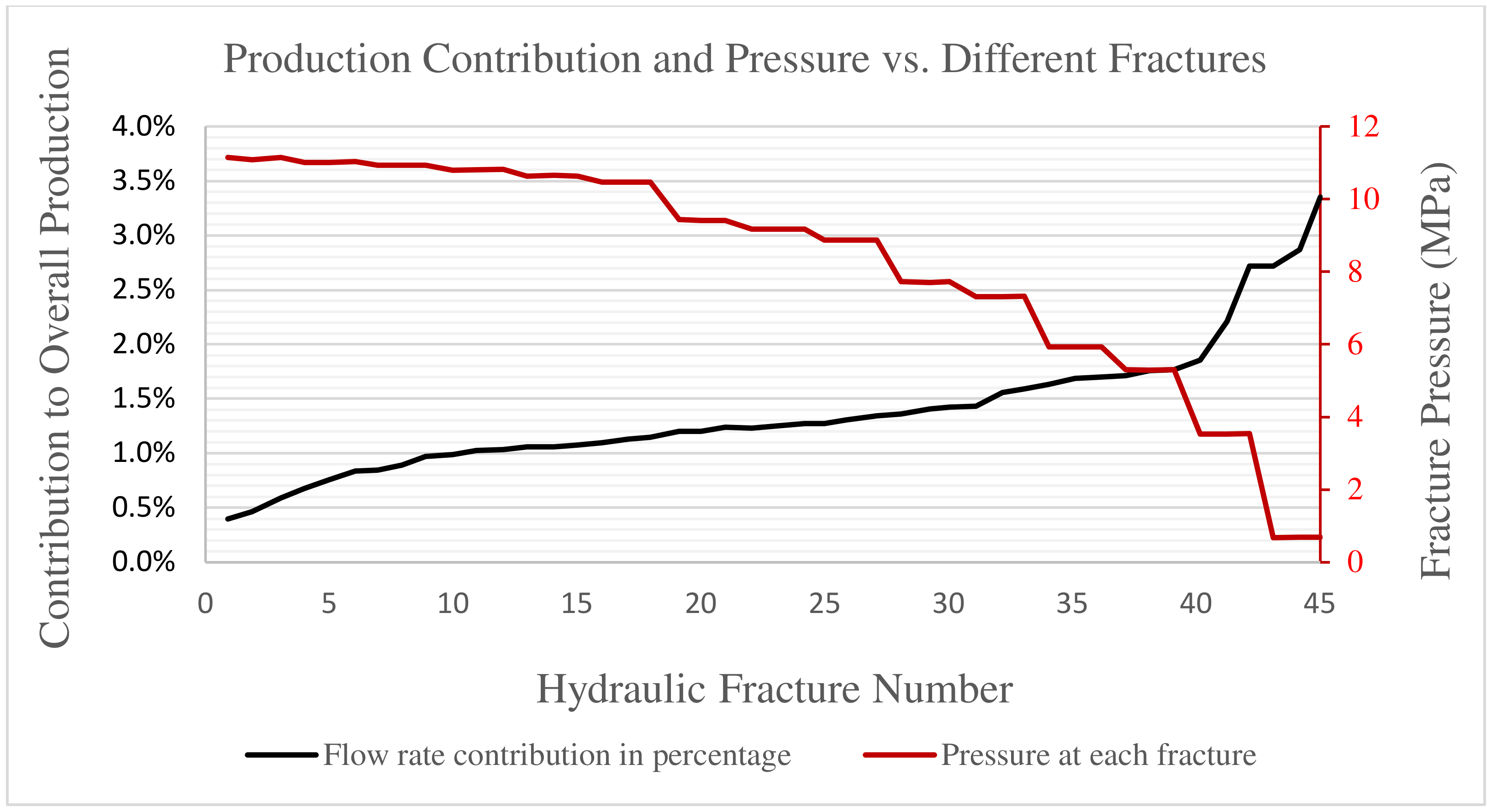
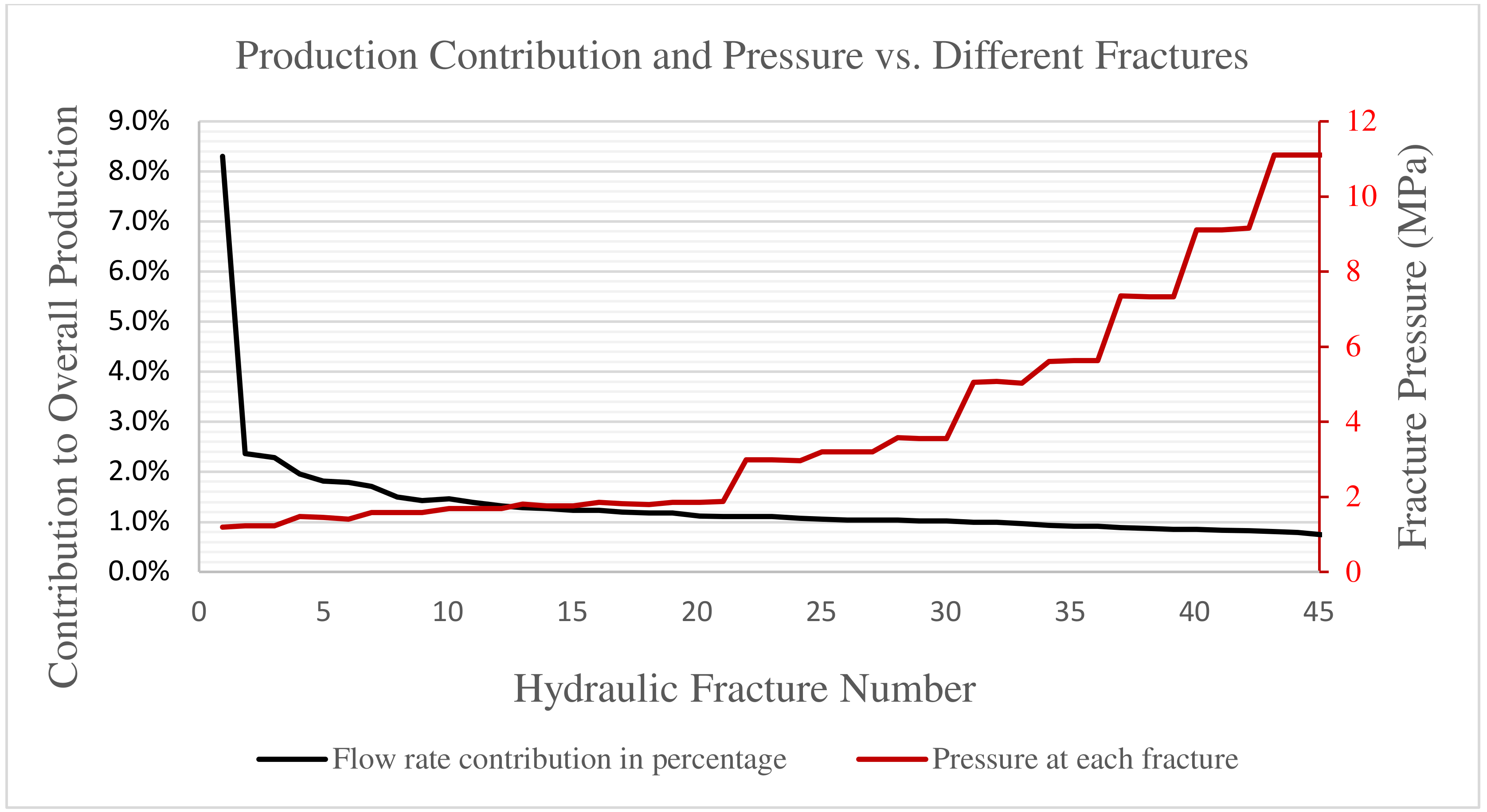
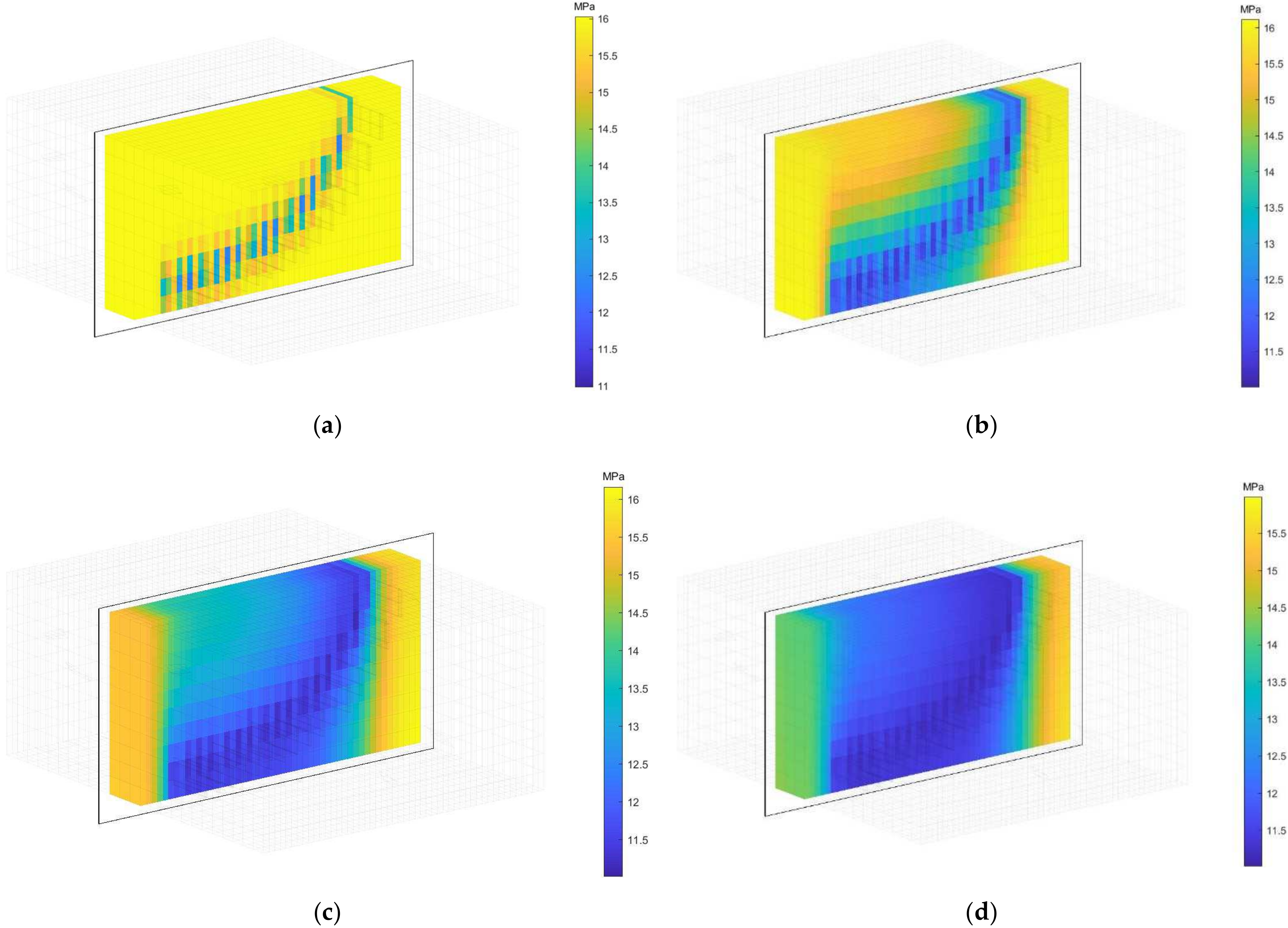
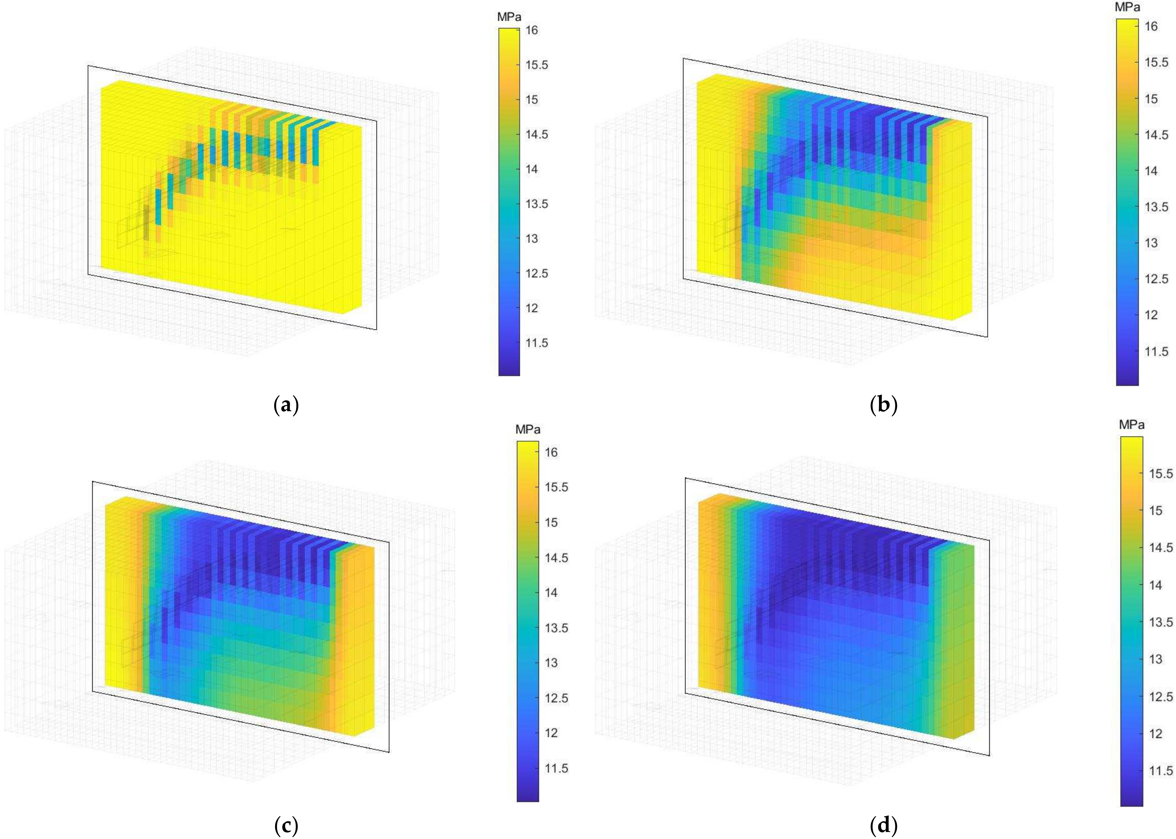
• The model was extended and applied to two examples with extreme well trajectories to explore the impact of trajectory in this level on well productivity. The pressure and flowrate at each fracture was calculated, and the latter was converted into the production contribution. By comparing pressure distribution to production contribution of each hydraulic fracture, the production contribution was found to be oppositely proportional to the fracture pressure.
• The model using a hilly-terrain well trajectory was compared to the one using a straight well trajectory. Though the percentage difference was less than 10% in most of the time steps, it should be noted that the case well had a depth difference less than 20 m in an overall 1500 m well length. In a case where the well has a depth difference over this value, and even exceeding 100 m in some scenarios, the effect of hilly-terrain well trajectory on well productivity should not be ignored.
• The simulated production data of the two cases was plotted together and compared. The tilt-up case well was found to have higher production due to the lower bottomhole pressure at shallower depths.

In conclusion, this model comprehensively considers the effects and inter-relationship of natural fractures, hydraulic fractures, and the hilly-terrain well trajectory, produces simulation results consistent with actual production conditions, and is expected to guide field design and operation in fracturing and drilling.

References

1. Smith, M.B.; Montgomery, C. Hydraulic Fracturing; CRC Press: Boca Raton, FL, USA, 2015. [Google Scholar]
2. Joshi, S.D. Horizontal Well Technology; OSTI: Washington, DC, USA, 1991. [Google Scholar]
3. Torres, F.; Xavier, M.; Ailin, J.; Yu, W.; Yunsheng, W.; Junlei, W.; Xie, H.; Li, N.; Miao, J. Comparison of dual porosity dual permeability with embedded discrete fracture model for simulation fluid flow in naturally fractured reservoirs. In Proceedings of the 54th U.S. Rock Mechanics/Geomechanics Symposium, Online, 28 June–1 July 2020. [Google Scholar]
4. Peaceman, D.W. Fundamentals of Numerical Reservoir Simulation; Elsevier: Amsterdam, The Netherlands, 2000. [Google Scholar]
5. Wang, G. Issues concerning application of horizontal well data in 3-d modeling of shale reservoirs. In Proceedings of the AAPG Annual Convention and Exhibition, Houston, TX, USA, 3 April 2017. [Google Scholar]
6. Da Silva, D.V.A.; Jansen, J.D. A review of coupled dynamic well-reservoir simulation. IFAC-PapersOnLine 2015, 48, 236–241. [Google Scholar] [CrossRef]
7. Liyong, L.; Lee, S.H. Efficient field-scale simulation of black oil in a naturally fractured reservoir through discrete fracture networks and homogenized media. SPE Reserv. Eval. Eng. 2008, 11, 750–758. [Google Scholar]
8. Kim, J.-G.; Deo, M.D. Finite element, discrete-fracture model for multiphase flow in porous media. AIChE J. 2000, 46, 1120–1130. [Google Scholar] [CrossRef]
9. Jiang, J.; Younis, R. An improved projection-based embedded discrete fracture model (pEDFM) for multiphase flow in fractured reservoirs. Adv. Water Resour. 2017, 109, 267–289. [Google Scholar] [CrossRef]
10. Dumkwu, F.A.; Islam, A.W.; Carlson, E.S. Review of well models and assessment of their impacts on numerical reservoir simulation performance. J. Pet. Sci. Eng. 2012, 82, 174–186. [Google Scholar] [CrossRef]
11. Sharma, Y.; Ihara, M.; Manabe, R. Simulating slug flow in hilly-terrain pipelines. In Proceedings of the SPE International Petroleum Conference and Exhibition in Mexico, Villahermosa, Mexico, 10–12 February 2002. [Google Scholar]
12. Zheng, G.H.; Brill, J.; Shoham, O. An experimental study of two-phase slug flow in hilly terrain pipelines. SPE Prod. Facil. 1995, 10, 233–240. [Google Scholar] [CrossRef]
13. Yang, Y.; Li, J.; Wang, S.; Wen, C. Gas-liquid two-phase flow behavior in terrain-inclined pipelines for gathering transport system of wet natural gas. Int. J. Press. Vessel. Pip. 2018, 162, 52–58. [Google Scholar] [CrossRef] [Green Version]
14. Shi, S.; Wu, X.; Han, G.; Zhong, Z.; Li, Z.; Sun, K. Numerical Slug Flow Model of Curved Pipes with Experimental Validation. ACS Omega 2019, 4, 14831–14840. [Google Scholar] [CrossRef] [PubMed]
15. Zheng, G.; Brill, J.P.; Shoham, O. Hilly terrain effects on slug flow characteristics. In Proceedings of the SPE Annual Technical Conference and Exhibition, Houston, TX, USA, 3–6 October 1993. [Google Scholar]
16. He, Z.; He, L.; Liu, H.; Wang, D.; Li, X.; Li, Q. Experimental and Numerical Study on Gas-Liquid Flow in Hilly-Terrain Pipeline-Riser Systems. Discret. Dyn. Nat. Soc. 2021, 2021, 5529916. [Google Scholar] [CrossRef]
17. Cerna, C.K.Q.; Moreno, R.B.Z.L. Condensate banking characterization using pressure transient analysis and numerical simulation. In Proceedings of the SPE Latin American and Caribbean Petroleum Engineering Conference, Quito, Ecuador, 18–20 November 2015. [Google Scholar]
18. Ali, J. Parametric study of gas condensate flow near the wellbore. In Proceedings of the Canadian International Petroleum Conference, Calgary, AB, Canada, 5–8 June 2000. [Google Scholar]
19. Ayala, L.F.; Ertekin, T.; Adewumi, M.A. Compositional modeling of retrograde gas-condensate reservoirs in multimechanistic flow domains. SPE J. 2005, 11, 480–487. [Google Scholar] [CrossRef]
20. Ghahri, P.; Jamiolahmady, M.; Sohrabi, M. Gas condensate flow around deviated and horizontal wells. In Proceedings of the SPE EUROPEC/EAGE Annual Conference and Exhibition, Vienna, Austria, 23–26 May 2011. [Google Scholar]
21. Moinfar, A.; Varavei, A.; Sepehrnoori, K.; Johns, R.T. Development of an Efficient Embedded Discrete Fracture Model for 3D Compositional Reservoir Simulation in Fractured Reservoirs. SPE J. 2014, 19, 289–303. [Google Scholar] [CrossRef] [Green Version]
22. Chen, Z.; Liao, X.; Zhao, X.; Dou, X.; Zhu, L.; Sanbo, L. A finite-conductivity horizontal-well model for pressure-transient analysis in multiple-fractured horizontal wells. SPE J. 2017, 22, 1112–1122. [Google Scholar] [CrossRef]
23. Zhang, D.; Dai, Y.; Ma, X.; Zhang, L.; Zhong, B.; Wu, J.; Tao, Z. An analysis for the influences of fracture network system on multi-stage fractured horizontal well productivity in shale gas reservoirs. Energies 2018, 11, 414. [Google Scholar] [CrossRef] [Green Version]
24. Kamyab, M.; Dejam, M.; Masihi, M.; Ghazanfari, M. The gas-oil gravity drainage model in a single matrix block: A new relationship between relative permeability and capillary pressure functions. J. Porous Media 2011, 14, 709–720. [Google Scholar] [CrossRef]
25. Peaceman, D.W. Interpretation of Well-block pressures in numerical reservoir simulation with nonsquare grid blocks and anisotropic permeability. Soc. Pet. Eng. J. 1983, 23, 531–543. [Google Scholar] [CrossRef]
26. Olorode, O.; Wang, B.; Rashid, H.U. Three-Dimensional Projection-Based Embedded Discrete-Fracture Model for Compositional Simulation of Fractured Reservoirs. SPE J. 2020, 25, 2143–2161. [Google Scholar] [CrossRef]
27. Rao, X.; Cheng, L.; Cao, R.; Jia, P.; Dong, P.; Du, X. A modified embedded discrete fracture model to improve the simulation accuracy during early-time production of multi-stage fractured horizontal well. In Proceedings of the SPE/IATMI Asia Pacific Oil & Gas Conference and Exhibition, Bali, Indonesia, 29–31 October 2019. [Google Scholar]
28. Lie, K.-A. An Introduction to Reservoir Simulation Using MATLAB/GNU Octave: User Guide for the MATLAB Reservoir Simulation Toolbox (MRST); Cambridge University Press: Cambridge, UK, 2019. [Google Scholar]
29. Stein, K. MRST-AD: An open-source framework for rapid prototyping and evaluation of reservoir simulation problems. In Proceedings of the SPE Reservoir Simulation Symposium, Houston, TX, USA, 23–25 February 2015. [Google Scholar]
30. Zhao, Y.; Lu, G.; Zhang, L.; Wei, Y.; Guo, J.; Chang, C. Numerical simulation of shale gas reservoirs considering discrete fracture network using a coupled multiple transport mechanisms and geomechanics model. J. Pet. Sci. Eng. 2020, 195, 107588. [Google Scholar] [CrossRef]
31. Tran, T.V.; Ngo, A.T.; Hoang, H.M.; Tran, N.H. Production performance of gas condensate reservoirs: Compositional numerical model—A case study of Hai Thach–Moc Tinh Fields. In Proceedings of the Abu Dhabi International Petroleum Exhibition and Conference, Abu Dhabi, UAE, 9–12 November 2015. [Google Scholar]
Figure 1. The case well trajectory with a hilly-terrain trajectory.
Energies 15 01854 g001
Figure 2. Case well demonstration with both hydraulic fractures and natural fractures.
Energies 15 01854 g002
Figure 3. Plot of oil production data with time.
Energies 15 01854 g003
Figure 4. Plot of gas production data with time.
Energies 15 01854 g004
Figure 5. Comparison of gas productions simulated by using different grid sizes and grid numbers.
Energies 15 01854 g005
Figure 6. Simulated gas production at different permeabilities.
Energies 15 01854 g006
Figure 7. Simulated gas production at different porosities.
Energies 15 01854 g007
Figure 8. Simulated gas production with different numbers of natural fractures.
Energies 15 01854 g008
Figure 9. Comparison between the hilly-terrain well trajectory case and the perfectly straight well trajectory, and the percentage difference between the two results plotted on the secondary y-axis.
Energies 15 01854 g009
Figure 10. Tilt-up well trajectory with a depth difference of 120m from the well’s starting point.
Energies 15 01854 g010
Figure 11. Tilt-up well demonstration with both hydraulic fractures (yellow rectangle) and natural fractures (gray rectangle); the well trajectory is represented by the red line.
Energies 15 01854 g011
Figure 12. Tilt-down well trajectory with a depth difference of 120 m from the well’s starting point.
Energies 15 01854 g012
Figure 13. Tilt-down well demonstration with both hydraulic fractures (yellow rectangle) and natural fractures (gray rectangle); the well trajectory is represented by the red line.
Energies 15 01854 g013
Figure 14. Pressure distribution and production contribution at each hydraulic fracture in the tilt-up well case.
Energies 15 01854 g014
Figure 15. Pressure distribution and production contribution at each hydraulic fracture in the tilt-down well case.
Energies 15 01854 g015
Figure 16. Plot of gas production data with time of the tilt-up well example.
Energies 15 01854 g016
Figure 17. Static pressure of the reservoir in tilt-up case at production time (a) day 2, (b) day 30, (c) day 90, and (d) day 360.
Energies 15 01854 g017
Figure 18. Plot of gas production data with time of the tilt-down well example.
Energies 15 01854 g018
Figure 19. Static pressure of the reservoir in tilt-down case at production time (a) day 2, (b) day 30, (c) day 90, and (d) day 360.
Energies 15 01854 g019
Figure 20. Comparison between two well examples with simulated production data.
Energies 15 01854 g020
Publisher’s Note: MDPI stays neutral with regard to jurisdictional claims in published maps and institutional affiliations.