Numerical and Experimental Investigation of the Effect of Design Parameters on Savonius-Type Hydrokinetic Turbine Performance

Abstract

To meet the increased demand of hydroelectric power generation, a novel drag-based Savonius turbine with the characteristics of a simpler fabrication process and good starting characteristics is designed, fabricated, and analyzed. The newly designed turbine is suitable to be installed in rivers, irrigation channels, ocean currents, etc., for small-scale hydroelectric power generation. In the present study, experiments are carried out to investigate the influence of the design parameters of this turbine on its power performance in order to improve its efficiency, including blade arc angles (180°, 135°), blade placement angles (0°, ±22.5°), and the number of blades (2, 3, 6, and 8). Further, three-dimensional CFD simulations are performed with Re = $6.72\times {10}^5$, matching the experimental conditions, in order to study the changes in the flow field and the rotation characteristics of the turbine. The research results indicate that a six-bladed turbine with a blade arc angle of 135° and a blade placement angle of 0° has higher torque and better power performance, which makes it the most suitable design when also considering cost. Furthermore, it was found that an increase in the number of turbine blades contributes to improving the performance of the turbine. The maximum power coefficient is 0.099 at a tip speed ratio of 0.34.

1. Introduction

Due to global warming [1], the global environment has changed in various ways since the industrial revolution because of damage to the environment and limitations in the amount of available fossil fuels [2,3]. The dependence of humans on electricity has become increasingly more serious with the growth of the population and economic results, so countries have begun to pay attention to the development and utilization of green energy, including biomass energy, geothermal energy, solar energy, hydropower, and wind energy [4,5]. Because water accounts for more than 75% of the earth’s surface, compared with other energy sources, hydropower is a cleaner and more predictable source, and generates lower ${\mathrm{CO}}_2$ emissions [6,7]. Therefore, water resources that harvest hydrokinetic energy from flowing rivers, tidal currents, ocean water currents, irrigation canals, or other artificial waterways are considered to be viable energy sources.

There are two categories of turbines used to harvest energy from water flow: non-turbine systems [8] and turbine systems. A turbine system includes the use of hydrostatic energy (potential energy) and hydrokinetic energy turbines to generate electricity. Among them, a hydrokinetic energy turbine uses the kinetic energy of natural water resources to replace potential energy to generate electricity, without using a water storage structure which leads to environmental damage.

According to the alignment of the axis of rotation relative to the direction of the water flow, there are mainly two technologies applied to hydrokinetic turbines: horizontal-axis turbines [9] and vertical-axis turbines [10]. Horizontal-axis turbines have an advantage in terms of tidal and wind energy, but for small-scale energy conversion they are not cost-effective [11,12]. Vertical-axis turbines are mainly divided into two types [13]: drag-based Savonius and lift-based Darrieus. The Savonius turbine was invented by a Finnish architect, Sigurd J. Savonius, for wind applications in 1920 [14]. It is an energy conversion device that uses the difference in resistance between concave blades and convex blades to convert energy.

Although Savonius turbines were originally used for wind power (SWT), water is 856 times denser than air, which has led researchers to study the potential of Savonius hydrokinetic turbines (SHTs) [15].

Furthermore, the fluid dynamic characteristics in the flow field around turbines are considerably different because of the fundamental difference between wind and water flow. Wind flow is mainly controlled by pressure differences, while water flow is mainly affected by gravity [16].

Although the power performance of the Savonius turbine 20% less that that of the lift-based turbine [17], it has many advantages, including being suitable for low velocity streams, a simple turbine structure, better self-starting characteristics, the ability to harness water flow from different directions, and being less noisy, which reduces the vibration and damage to the turbine structure [18]. In addition, maintenance costs are low because the power equipment can be installed above the water.

In recent years, many researchers have proposed various numerical and experimental methods to improve Savonius hydrokinetic turbine (SHT) technology. The aspect ratio, the overlap ratio, the blade profile, the number of blades, and deflectors are the main factors that directly affect the efficiency of SHTs.

Reviews on the early stages of research on vertical axis Savonius turbines all focused on wind energy. Blackwell et al. [19] proposed that increasing the Reynolds number and aspect ratio would improve performance. Sivasegaram et al. [20] investigated the performance of different blade numbers, shapes, sizes, and positions. According to the literature, the Reynolds number, the wake aspect ratio, the size of the end plate and the shaft diameter all influence turbine performance. Kahn [21], Ushiyama, and Nagai et al. [22] studied the effects of the aspect ratio of the rotor, the shape of the rotor, the overlap, and separation gap between the rotor blades, the profile of the blade cross section, and the number of blades on the performance characteristics. Fujisawa and Gotoh [23] tested the pressure distribution on the blade surface under various rotor angles and tip speed ratios to research the aerodynamic performance of the Savonius turbine. Sheldahl et al. [24] experimentally tested the performance of two- and three-bladed SWTs. Their tests revealed that, compared with the three-bladed turbine, the $C_p$ value for the two-bladed turbine was approximately 1.5 times higher than that for the three-bladed turbine. Emmanuel et al. [25] demonstrated that the performance of the six-bladed SWT is better than that of the two-bladed SWT. According to the results of a CFD simulation, the power coefficient is expected to increase from 0.25 to 0.3. (If a deflector was installed in the six-bladed SWT, this could be increased to 0.5.) Mahmoud et al. [26] developed a two-bladed turbine that is more efficient than both a three-bladed turbine and four-bladed turbine, where a rotor with end plates was found to be more efficient than a rotor without end plates. Compared with a single-stage rotor, a two-stage rotor had better performance. A rotor without an overlap ratio performed better than a rotor with an overlap ratio in terms of operation. The results also showed that the power factor increased with the aspect ratio. Wenehenubun et al. [27] found that, compared with two-bladed and four-bladed wind turbines, three-bladed wind turbines have higher rotational speeds and tip speed ratios. Compared with two-bladed or three-bladed wind rotors, four-bladed wind turbine rotors had higher torque; four-bladed wind turbines had good performance at lower tip speed ratios, but three-bladed wind turbines had the best performance at higher tip speed ratios. Banerjee [28] and Alom [29] used experiments and simulations to study elliptical blades. The results indicated that the flow characteristics of the elliptical blade turbine were better than the traditional semicircular design. Khaled R.Abdelaziz et al. [30] studied the effect of adding curved and straight auxiliary blades at the turbine blade on the performance of the Savonius turbine numerically.

In the past decade, research on Savonius hydrokinetic turbines (SHT) has made great progress.

Faizal et al. [31] designed the five-bladed Savonius and studied how orbital motion in waves affected the energy extracted by SHT. Increasing both wave height and frequency amplifies the speed of the turbine, according to their results. As a result of this, the performance of SHTs is determined by their design parameters and the surrounding fluid behavior. Yaakob et al. [32] analyzed the performance of a two-bladed semicircular SHT in two- and three-dimensional simulations with a constant current velocity of 0.56 m/s and reported a $C_{pmax}$ of 0.275 at a TSR = 0.7, which validated the experimental results. In 2011, Kailash Golecha et al. [12] tested two stage and three stage modified Savonius rotors for a hydrokinetic turbine to study the influence of the deflector plate at the optimal position. Deflection plates for two-stage deflection plates for two-stage 0° phase shifts, 90° phase shifts, and three-stage modified Savonius rotors have each seen significant increase in power coefficient of 42%, 31%, and 17% respectively. In addition, this study investigated whether by placing the deflector appropriately upstream of the river, the performance of the Savonius rotor could be significantly improved. Sarma et al. [15] examined a three-bladed turbine in an open channel at a water velocity of 0.3–0.9 m/s. The test revealed that a $C_{pmax}$ of 0.39 at TSR = 0.77. Compared with the conventional SWT under the same input value, this was 61.32% higher. Khan et al. [33] studied the performance of single-stage, two-stage and three-stage semicircular blade SHTs. The $C_{pmax}$ value of the two-stage rotor was approximately 0.5, which was approximately 4% better performance than that of single-stage and three-stage rotors. However, these differences were small, which indicates that the rotor should be selected based on the simplicity of the structure rather than the power output. Golecha et al. [34] investigated whether a straight arc shape leads to a higher power coefficient. The study also showed that the use of deflection plates on both the advancing blade side and the returning blade side improved the performance of the Savonius rotor.The impact of overlap ratios and aspect ratios on performance of Savonius turbines in an open channel was studied by Patel et al. [35]. The results showed that the $C_p$ value for an overlap ratio was approximately 0.11 for Savonius turbines, where the maximum aspect ratios less were than 0.6. Kumar and Saini [36] investigated the influence of twist angle and Reynolds numbers on the hydrokinetic performance of a Savonius turbine. A numerical simulation was carried out using ANSYS Fluent in their study. A $C_{pmax}$ of 0.39 at a TSR = 0.9 was obtained for a given water velocity of 2 m/s. Parag K et al. [37] studied the performance of SHTs through experiments and CFD. The performance of two- and three-bladed SHT, as well as elliptical blade and semi-circular blades, is compared. The results showed that the performance of two-bladed and semi-circular blade SHT was better than that of other alternatives. Mabrouk M et al. [38] investigated the performance of the Helical Savonius in irrigation channels. An improved deflector system design was proposed in order to enhance the performance of the studied water turbine. Fen G et al. [39] researched the influence of a rear deflector on a Savonius turbine with a towing box experiment and a two-dimensional simulation. Although deflector devices can improve the performance of an SHT [12,34,39], the additional equipment also make the entire turbine system more complicated.

1.1. Motivation

Wind and water are currently the two most common energy sources for Savonius turbines; however the flow field performance of open channel water flow differs considerably from wind. Water flow is controlled by gravity, while wind is mainly influenced by pressure differences. In addition, researchers are interested in the higher power density of water to study the potential of SHT. Therefore, this study is aimed toward modifying the design parameters of SHTs to improve their performance. In previous literature on SWTs, there have been different opinions on the optimal number of blades. Some studies [24,26,37,40] have shown that two blades provide better performance efficiency than three blades. However, some studies have suggested that more than two blades will lead to better performance [25,27,29]. The above results were based on the findings related to SWTs, but there are still few studies examining the effects of the number of blades on SHT performance, thus, an evaluation of this parameter is necessary.

1.2. Present Objective

The literature on SWTs has discussed many different types of blades, but SHT studies have mostly discussed only semi-circular blades. In this study, an attempt is made to change the shape and angle of the blades to observe the efficiency of the turbine and verify the results through experiments and simulations. In brief, the novelty of this research lies in the experimental testing of the effects of the number of blades and blade shape on SHTs. First, six-bladed SHTs with arc angles of 135° and 180° (semi-circular) are tested to find the best blade shape based on the power coefficient. Subsequently, the six-bladed SHT with a 135° arc angle is tested with different placement angles of 0° and ±22.5° in the experiments. Further, SHTs with two, three, six, and eight blades were tested to find the optimal blade shape and number. In order to obtain a deeper understanding of the hydrodynamic performance and flow field changes of the SHT, CFD simulations using ANSYS-CFX were carried out.

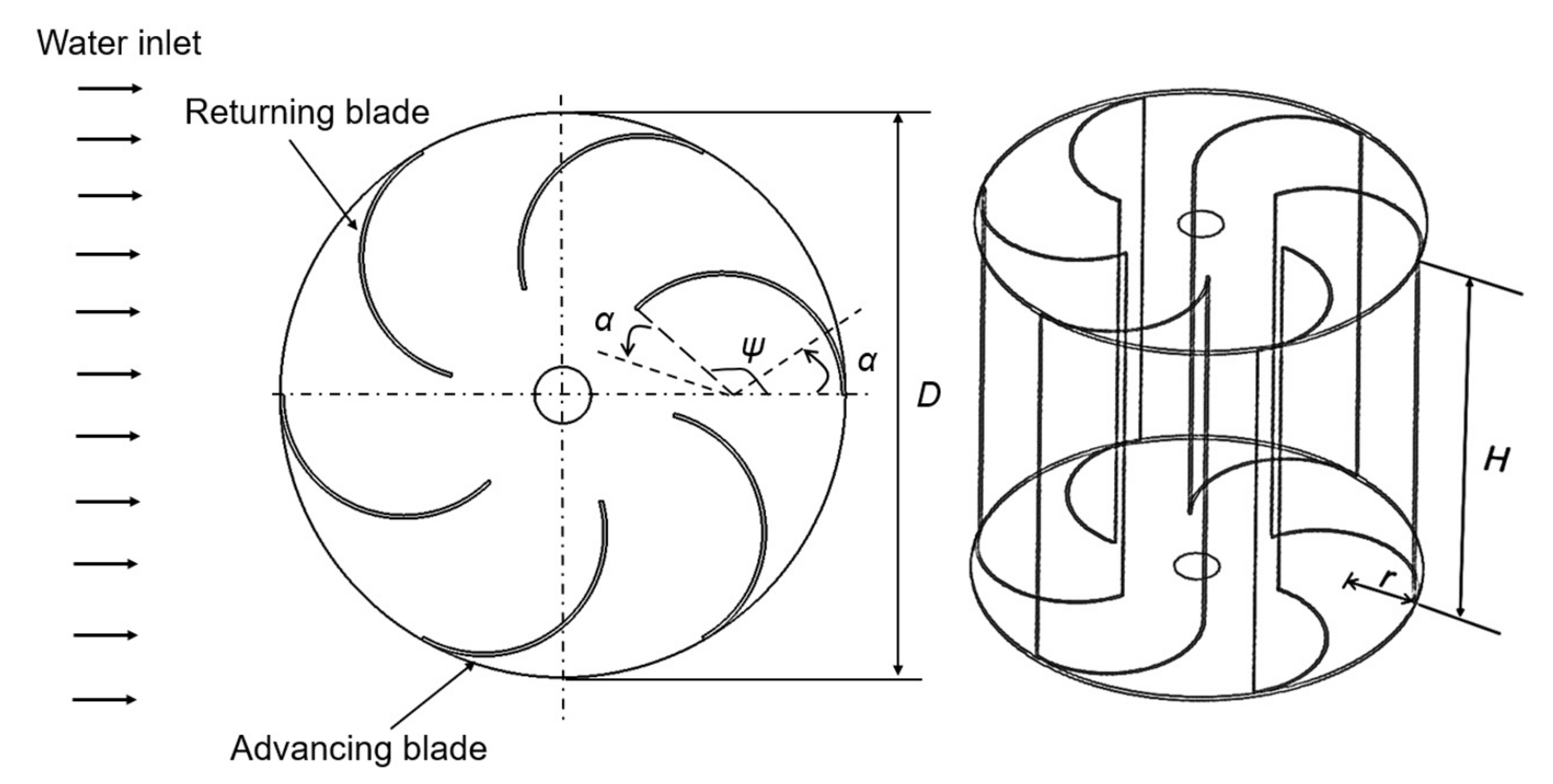
2. Turbine Design and Performance Parameters

The parameters that influence the performance of a vertical drag hydrokinetic turbine include the aspect ratio, blade shapes, number of blades, and end plates. The aspect ratio (AR) has an important influence on efficiency performance, application location, structural capacity and power demand of the turbine, and it is typically expressed by the following equation:

$$AR=\frac{H}{D}$$

(1)

where H and D represent the turbine height and diameter, respectively. A lower aspect ratio (AR < 1.5) cause the turbine to have a more stable structure and greater stability [37]. In this study, the turbine is design with an AR = 1, for which the design parameters are shown in Figure 1. A hydrokinetic turbine with blades having two different profiles is considered for the analysis using blades with arc angles ($\psi$) of 180° and 135°, as shown in Figure 2. Each blade includes a concave and convex profile and is divided into an advancing blade and a returning blade according to the rotation. The pressure difference between the concave and convex surfaces of the blades is used to drive the turbine to rotate. In order to reduce the effect of the vortex inside the turbine and allow water to flow smoothly through the turbine, the blade arc angle ($\psi$) is designed to be 135°. The turbine blades are 3.75 mm thick. The height (H) and diameter (D) of the turbine are both 600 mm. In this study, the blade placement angles were varied to investigate their influence on the performance of the turbine. The dimensions of the blade placement angles ($\alpha$) are −22.5°, 0°, and +22.5°, as shown in Figure 3. In addition, several blades were developed with the same specifications ($\psi$ = 135°, $\alpha$ = 0°) to study the effect of the number of blades on the efficiency of a turbine, as shown in Figure 4.

Data Reduction

To evaluate the performance of water turbines, dimensionless coefficients are typically used. The most commonly used evaluation characteristic coefficients include the following: For open channels, the Reynolds number based on the rotor diameter is given by:

$$Re=\frac{\rho VD}{\mu }$$

(2)

where $\rho$ is the density of water; V is the free stream velocity; D is the rotor diameter; and $\mu$ is the viscosity of water.

The power coefficient of the turbine represents the ratio of the mechanical power produced by the turbine to the actual water kinetic energy available in the same area covered by the turbine [41], which is defined as follows:

$$C_p=\frac{T\omega }{\frac{1}{2}\rho A{V}^3}=\frac{P_{output}}{P_{available}}$$

(3)

where T is the torque produced by the turbine; $\omega$ is the angular velocity; and A is the projected turbine area.

The tip speed ratio is given by the following expression:

$$TSR=\frac{R\omega }{V}$$

(4)

where R is the turbine radius.

The turbine moment coefficient is defined by the following equation:

$$C_m=\frac{T}{\frac{1}{2}\rho AR{V}^3}$$

(5)

The blockage ratio is given by the expression below. When the blockage ratio is less than 30%, the performance of the turbine is less affected by the boundary effect [42]. The blockage rate in this study is 8%.

$$BR=\frac{frontalareaoftheobject}{crossSectionofthetunnel}$$

(6)

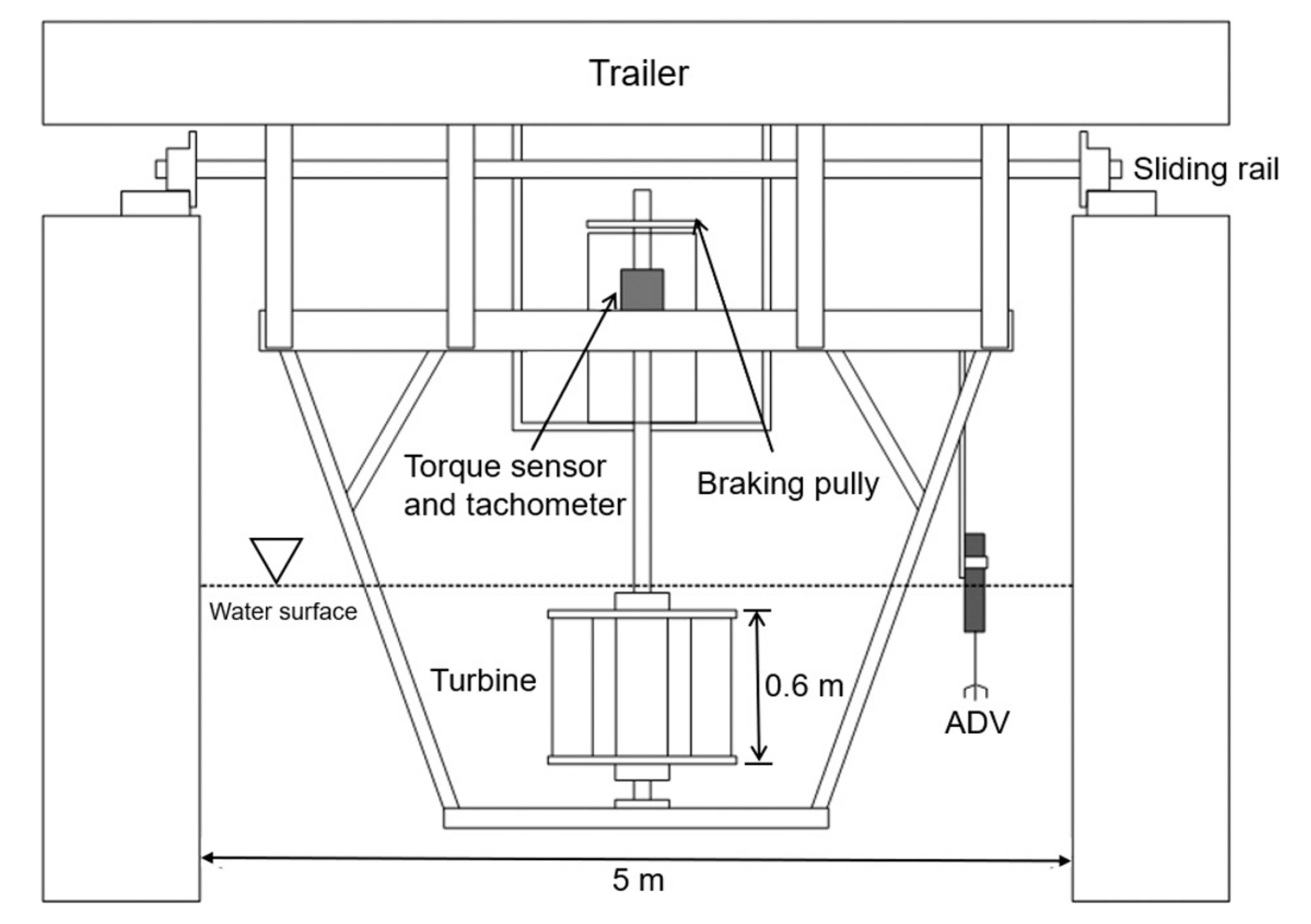
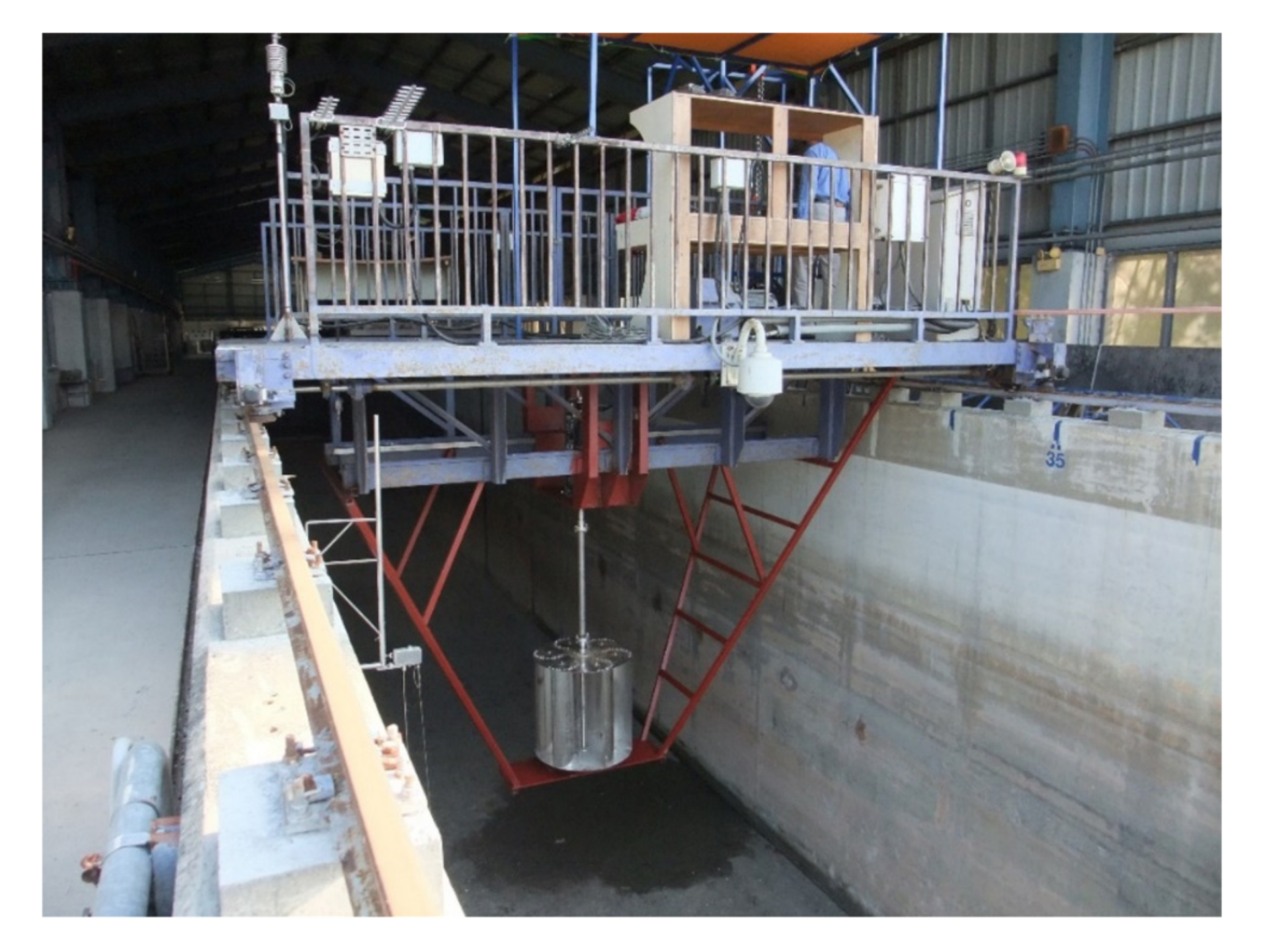
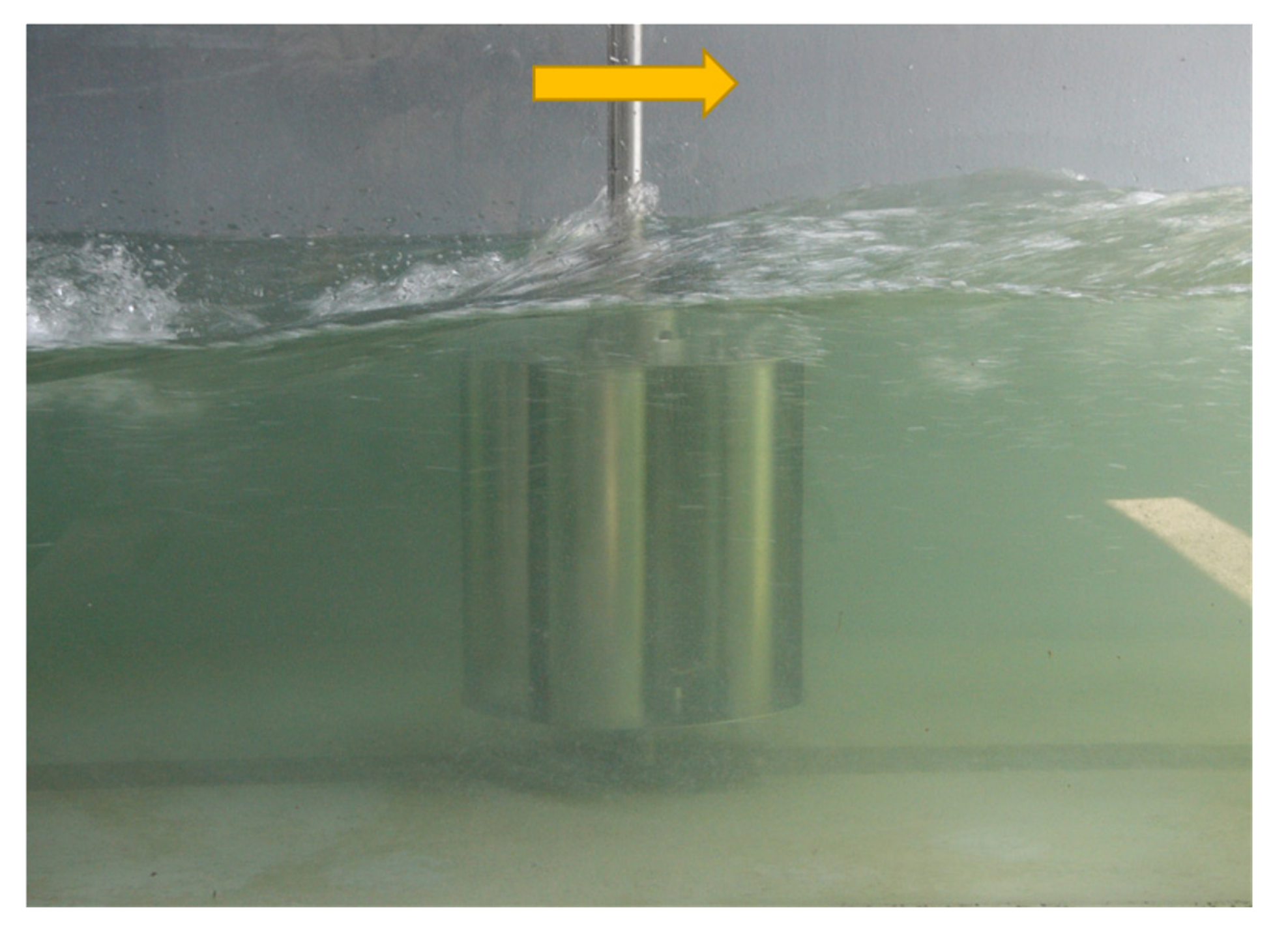
3. Experimental Methodology

The turbine material settings and experiment model were all made of stainless steel. The turbine proposed in this study was considered to be able to actually operate and generate electricity, so a large turbine (60 cm × 60 cm) was used in the scale. However, due to the limitation of the site, it was difficult to conduct experiments. A towing tank test platform [33,39,43] was set up to conduct the experiments. The width of the towing tank was approximately 5 m, and the turbine was fully immersed. The depth of water in the towing tank was 0.9 m, and the distance from the water surface to the top of the turbine was approximately 15 cm. In order to measure the torque and rotational speed generated by the turbine, a torque sensor with an accuracy of ±1% and a tachometer with an operating range of 10–29,999 RPM and accuracy of ±0.05% were mounted on the towing tank experimental platform, as shown in Figure 5 and Figure 6. The setup consisted of trailer, a sliding rail, a braking pulley, and an acoustic Doppler velocimeter (ADV), which was used to measure the velocity of the water flow. The trailer drove the turbine to move forward and rotate at a fixed speed of 1 m/s by the slide rail and also drove the relative movement of the turbine and the water flow, so it successfully simulated the impact of the water flow on the turbine. Because the position of the turbine was driven by the trailer moving forward, the turbine was not affected by the size of the tank or the backflow caused by the water hitting the wall. The trailer was set to 1 m/s, corresponding to Re = $6.72\times {10}^5$. The flow states were turbulent. Figure 7 shows the rotation of the turbine in the towing tank. This paper is to study the performance of the Savonius-type hydrokinetic turbine. The amount of hydrokinetic energy contained in flowing water current depends on the water velocity. Therefore, it can be known from the definition of the power coefficient, the actual water kinetic energy captured by the turbine is dominated by the free stream velocity and the free flow cross-sectional area, not by the height of the effective head, as shown in Equation (3). Moreover, the cross-sectional area of water passing through the turbine is affected by the height of the upstream water surface rather than the downstream water surface. Therefore, the water depth is determined when the turbine is stationary in this study In the experimental setup, the depth of the water is ensured so that the entire turbine is submerged in water during operation. The main purpose is to study and discuss the operation and flow field changes of the turbine as a whole immersed in the water.

4. Computational Methodology

Turbines will cause a vortex and wake region disturbance phenomenon when rotating, so it is impossible to clearly observe the changes in the water flow experimentally. In order to solve this problem, CFD is a very suitable tool. For an axisymmetric flow field, two-dimensional modeling can be used to calculate the flow field changes simply and quickly [43,44,45,46], or three-dimensional modeling can be used for more complex and real calculations to improve accuracy. Many previous studies only discussed dynamic simulations by giving the turbine a fixed angular velocity to facilitate rapid calculation [25,47], but there was a lack of important data for the turbine startup phase. Therefore, in this study, the passive rotation of the turbine for a three-dimensional CFD model under the impact of water flow is examined in order to capture continuous changes in the flow field.

4.1. Governing Equations

In the present study, the CFX flow solver is used to solve the Navier–Stokes equations and turbulence model with finite volume method discretization in order to deal with viscous incompressible turbulent flow field problems, where the body force is considered. Semi-Implicit Methods for Pressure-Linked Equation (SIMPLE) is used for the pressure-velocity coupling with second order upwind scheme. Convergence criteria are set at ${10}^{-5}$ for RMS residuals equations of momentum, continuity and turbulence characteristics.The details of the computational settings are shown in

Table 1. Details of the computational settings.

Characteristic	Value
Spatial discretization method	Finite Volume Method (FVM)
Convergence criteria for residuals	${10}^{-5}$
Turbulence model	Standard k-$ϵ$
Skewness	0.58

. The continuous equations and momentum equations are as follows [48,49]:

$$\frac{\partial \left(\rho \right)}{\partial t}+\frac{\partial \left(\rho u_j\right)}{\partial x_j}=0$$

(7)

$$\begin{array}{cc}\hfill \frac{\partial (\overline{\rho u_i)}}{\partial t}+\frac{\partial (\overline{\rho u_i{u}_j)}}{\partial x_j}=-\frac{\partial \left(\overline{p}\right)}{\partial x_i}+\frac{\partial }{\partial x_i}\left[\mu \right(\frac{\partial {\overline{u}}_i}{\partial x_j}+\frac{\partial \overline{u_j}}{\partial x_i}& \\ \hfill -\frac{2}{3}{\delta }_{ij}\frac{\partial {\overline{u}}_m}{\partial {\overline{x}}_m}\left)\right]+\frac{\partial }{\partial x_j}(-\overline{\rho u_i^{\prime }{u}_j^{\prime }})\end{array}$$

(8)

The Boussinesq’s gradient transport hypothesis is used to convert the Reynolds stress term into the relationships among the average flow velocity gradient.

$$-\rho \overline{u_i^{\prime }{u}_j^{\prime }}={\mu }_t(\frac{\partial \overline{u_i}}{\partial x_j}+\frac{\partial \overline{u_j}}{\partial x_i})-\frac{2}{3}(\rho k+{\mu }_t\frac{\partial {\overline{u}}_m}{\partial {\overline{x}}_m})$$

(9)

where ${\mu }_t$ is the turbulent viscosity, which is defined as:

$${\mu }_t=\rho \frac{C_{\mu }{k}^2}{ϵ}$$

(10)

where $\rho$ is the density; k is the turbulent kinetic energy; $ϵ$ is the Turbulent dissipation rate; and $C_{\mu }$ is the constant of the standard k-$ϵ$ turbulence model.

4.2. Turbulence Modelling

The flow field around the rotation of the turbine creates high levels of turbulence in nature. In order to simulate actual flow field performance, the choice of turbulence is very important, so a turbulent flow with a Reynolds number approximately $6.72\times {10}^5$ was used in this study. Many previous studies have used the standard k-$ϵ$ turbulence model for simulations [15,50,51,52], so the standard k-$ϵ$, which contains two semi-empirical equations, is used in this study. This two-equation semi-empirical model can be expressed as:

• Turbulent kinetic energy, k

  $$\begin{array}{cc}\hfill \frac{\partial \left(\rho k\right)}{\partial t}+\frac{\partial \left(\rho k{\mu }_i\right)}{\partial x_i}=\frac{\partial }{\partial x_j}\left[(\mu +\frac{{\mu }_t}{{\sigma }_k})\frac{\partial k}{\partial x_j}\right]+G_k-G_b& \\ \hfill -\rho ϵ-Y_M+Sk\end{array}$$

  (11)
• Turbulent dissipation rate, $ϵ$

  $$\begin{array}{cc}\hfill \frac{\partial \left(\rho ϵ\right)}{\partial t}+\frac{\partial \left(\rho ϵ{\mu }_i\right)}{\partial x_i}=\frac{\partial }{\partial x_j}\left[(\mu +\frac{{\mu }_t}{{\sigma }_{ϵ}})\frac{\partial k}{\partial x_j}\right]+C_{1ϵ}\frac{ϵ}{k}(G_k& \\ \hfill +G_{2ϵ}{G}_b)-C_{2ϵ}\rho \frac{{ϵ}^2}{k}+Sϵ\end{array}$$

  (12)

  where ${\sigma }_{ϵ}$ is the turbulent Prandtl number for $ϵ$; ${\sigma }_k$ is the turbulent Prandtl number for k; $G_k$ is the turbulent kinetic energy generation due to the mean velocity gradient; $Y_M$ is the effect of changes in dilatation of the compressible turbulence on the overall dissipation rate; and $G_b$ is the generation of turbulence kinetic energy due to buoyancy. In the above equation, $C_{\mu }$, $C_{1ϵ}$, $C_{2ϵ}$, ${\sigma }_{ϵ}$, and ${\sigma }_k$ are empirical coefficients, for which the values are as follows: $C_{\mu }$ = 0.09, $C_{1ϵ}$ = 1.44, $C_{2ϵ}$ = 1.92, ${\sigma }_{ϵ}$ = 1.3, and ${\sigma }_k$ = 1.0.

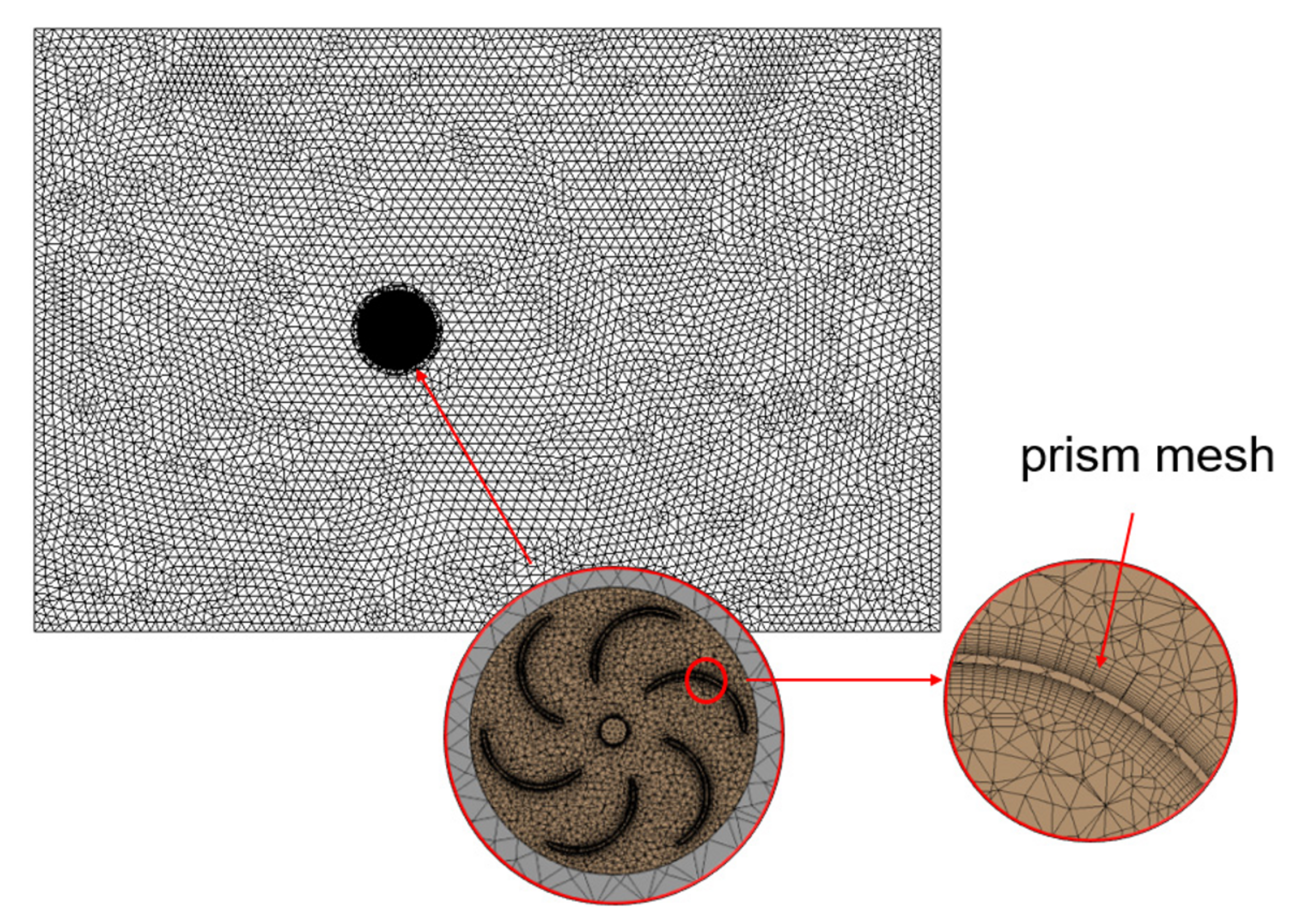
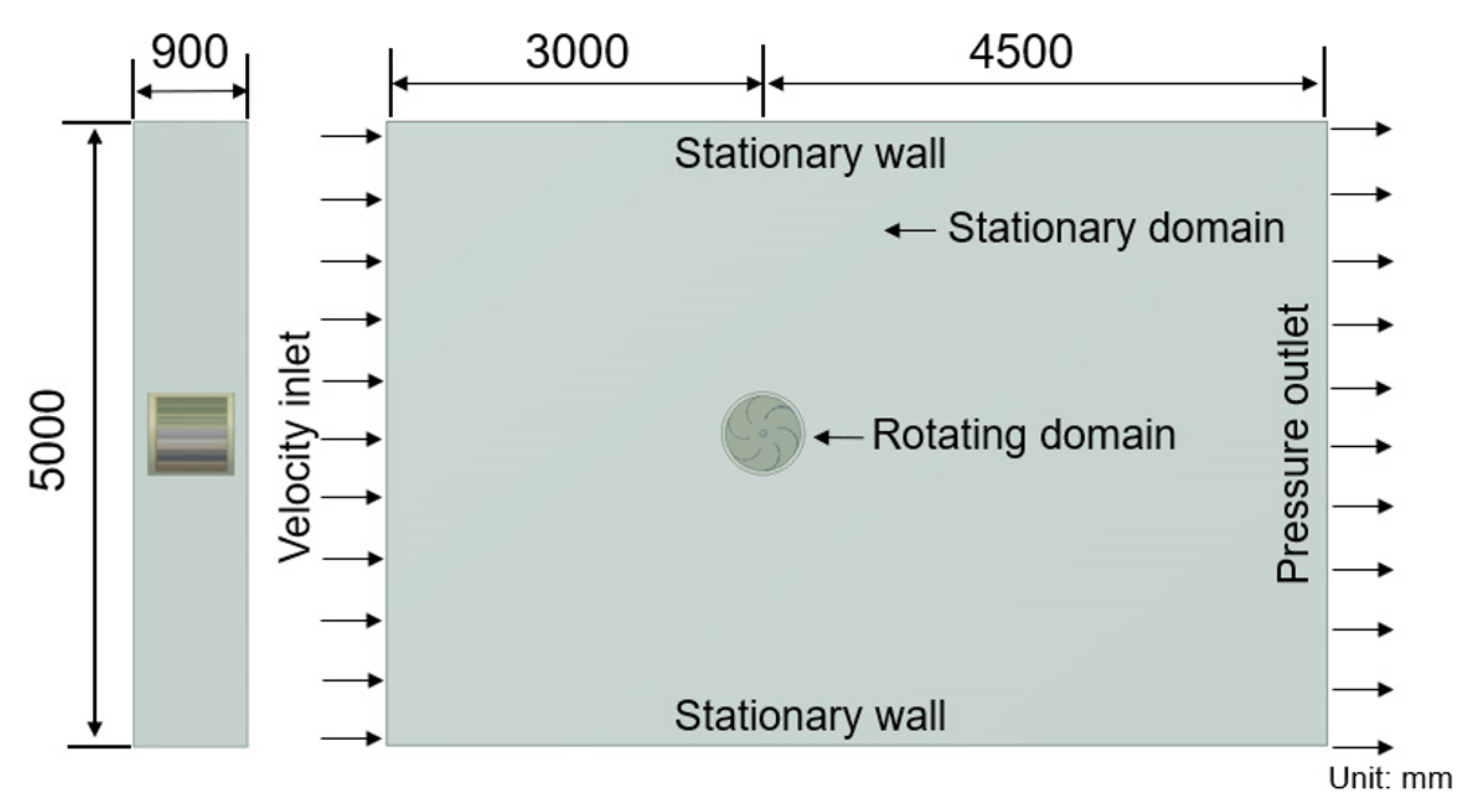
4.3. Computational Domains and Boundary Settings

The overall three-dimensional computational domains were mainly divided into rotating domain and stationary domain. The rotating domain contains turbines, and the other domains were stationary domains. Since in the experiment, the trailer setting method is used, the turbine will not be affected by the disturbed water flow generated after hitting the wall and will thus not affect the efficiency performance. Therefore, in terms of the simulation, for the basin, no-slip wall surfaces have been used. This design ensures that the water flow hitting the wall surface will not bounce back to the turbine and affect its rotation. After the water flow hits the wall surface, the velocity on the wall surface is 0, and the water flow moves along the wall surface and away from the turbine, which is the same as concept for the experimental setup. The computational domains are set to be the same as those used in the experiment, for which the total length is 7.5 m, which is 12.5 times the diameter of the turbine, and the domain width is 5 m, which is 8.3 times the diameter of the turbine. A velocity of V = 1 m/s is set at the inlet, and a pressure outlet is set at the downstream outlet, which ensures that the upstream and downstream pressures are the same. The rest of the walls are all set to the boundary conditions of the stationary wall, which are adiabatic boundaries and do not affect any condition of the fluid in the analysis, as shown in Figure 8.

4.4. Grid Independence Test

The ideal grid design should consider the characteristics of the flow field and the computer performance to select the appropriate grid size and perform partial mesh refinement processing in the rotating area. Because of the complex geometry of the turbine, an unstructured tetrahedron mesh was used to create the mesh for the entire domain. However, considering that the viscosity of the fluid near the solid boundary layer changes significantly, for the surface of the turbine blade, a structured prism mesh was adopted. The inflation layer of the blade surface boundary layer consisted of the prism mesh with a first layer thickness of 0.5 mm and a maximum of 10 layers with a growth rate of 1.2, as shown in Figure 9. In the CFD simulation, the independence of the mesh had to be analyzed first. As shown in

Table 2. Variations in $C_{pmax}$ relative to different amounts of elements.

Number of Elements in the Rotating Zone	Number of Elements in the Fixed Zone	Total Elements	${\mathit{C}}_{\mathbf{pmax}}$
240,088	16,638	256,726	0.0731
364,272	23,106	387,387	0.0812
627,904	32,654	660,558	0.0872
836,707	40,905	877,612	0.0924
1,010,098	83,675	1,093,934	0.0979
1,465,038	160,895	1,625,934	0.0984
2,261,104	285,966	2,547,070	0.0978

, a total of 7 sets of grid numbers ranging from 256,726 to 2,547,070 with average skewness of 0.58 which were generated to analyze the effect of the mesh number on the performance of the turbine and the hydrodynamic characteristics around the turbine. As the number of mesh elements increased from 256,726 to 1,093,773, the value of $C_p$ continued increased. However, when the number of mesh elements increased from 1,093,773 to 2,547,070, the $C_p$ value did not change to any significant degree. Therefore, 1,093,773 has indicated the convergence had been reached. In order to reduce the calculation costs, the total mesh number was set at 1,093,773 for the simulation.

5. Results and Discussion

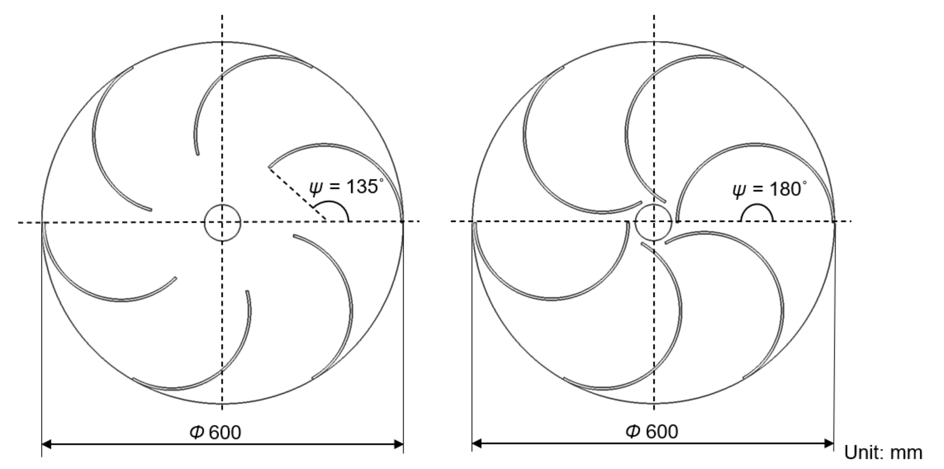
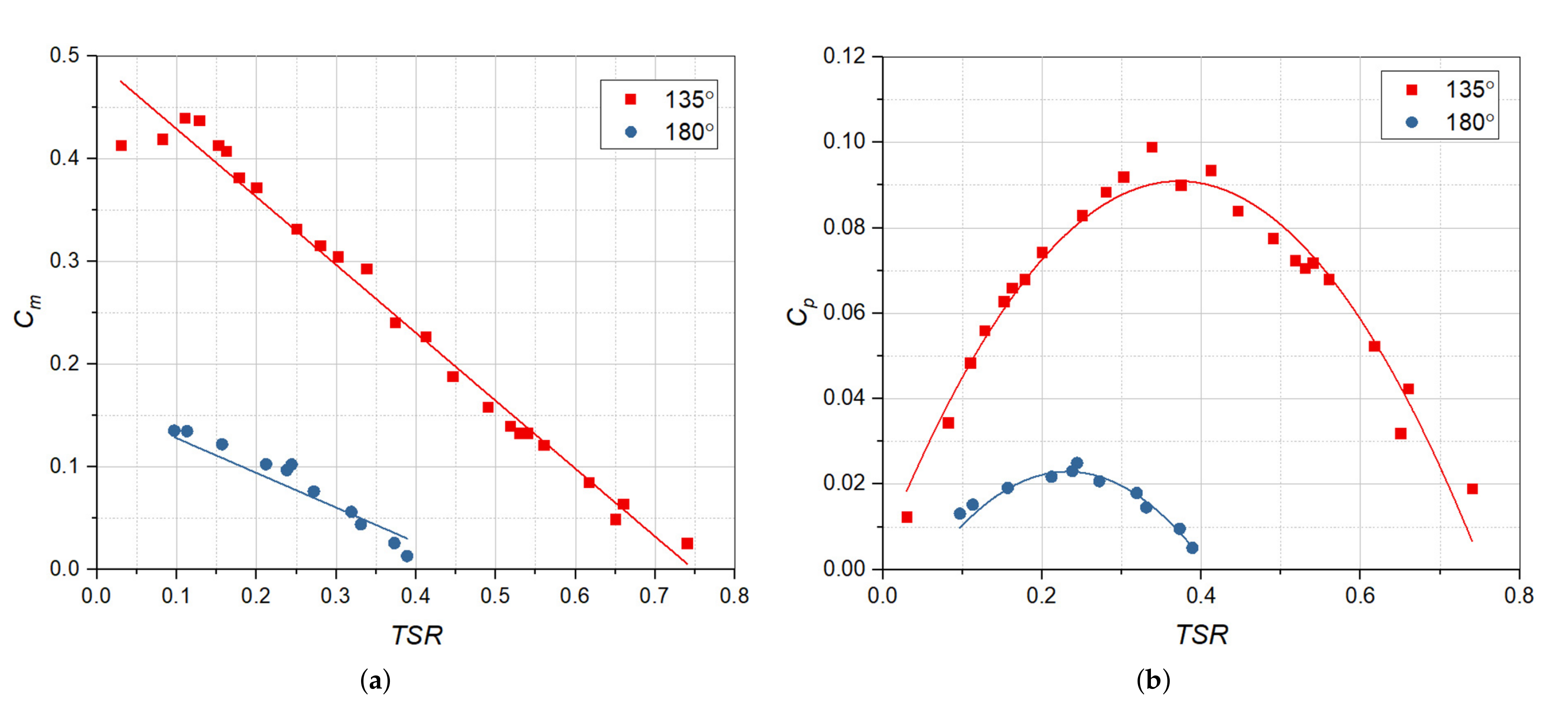
5.1. Effect of Blade Arc Angles ($\psi$)

Many studies have pointed out that the shape of the blade has a great influence on the output power of a turbine [53,54]. First, the difference in the measured efficiency of the 6-bladed turbine ($\alpha$ = 0°) is discussed when the blade arc angles were 180° and 135°. As shown in Figure 10, the moment coefficient and the power coefficient were calculated to correspond to the TSR to evaluate the efficiency of the turbine. Without applying load, the TSR for a blade arc angle of 135° was approximately 0.75, which was 0.4 greater than that obtained for a blade arc angle of 180°, as shown in Figure 10a. Additionally, as the mechanical load increased, the rotational speed of the turbine decreased and at the same time, the torque generated by the turbine increased, so the $C_m$ of the 135° blade arc angle was greater than that for a blade arc angle of 180°. Furthermore, it can be seen that the $C_p$ value and TSR exhibited a quadratic curve. Figure 10b shows a $C_{pmax}$ of 0.099 at a TSR of 0.34 when the blade arc angle was 135°, and a $C_{pmax}$ of 0.0249 at a TSR of 0.244 when the blade arc angle was 180°. It is obvious that the blade arc angle of 135° had better efficiency performance because the increase in the vorticities decreased the hydrodynamic performance of the turbine.

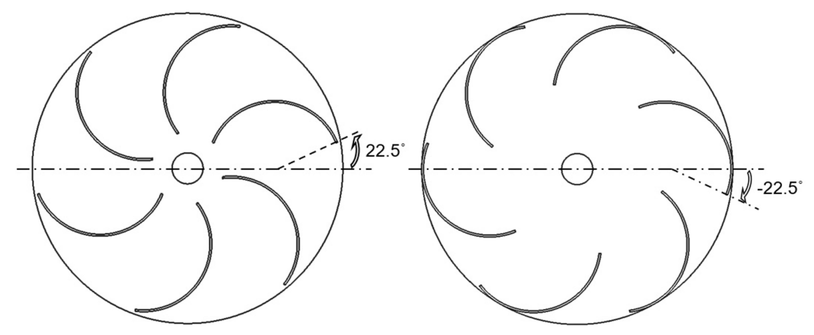
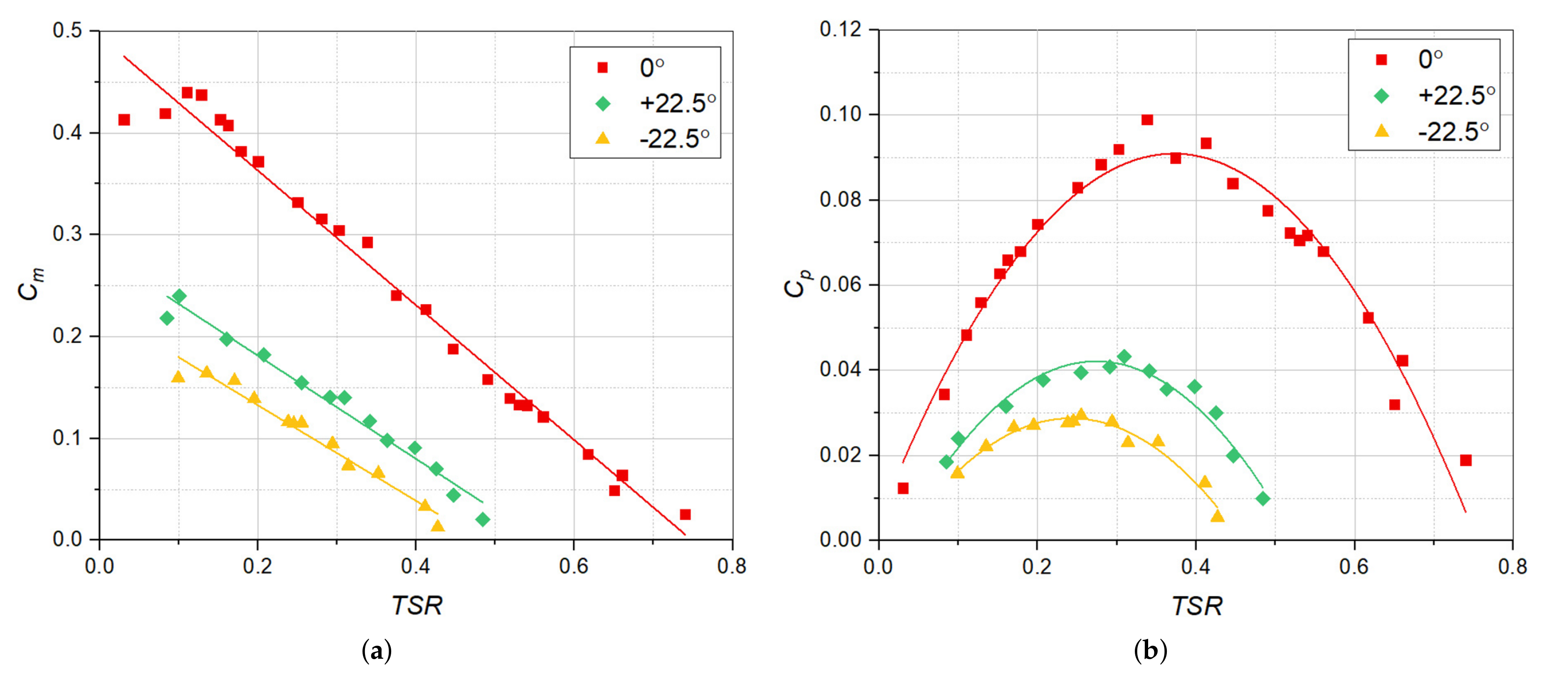
5.2. Effect of the Blade Placement Angles ($\alpha$)

From the previous section, it is known that when the blade arc angle is 135°, the efficiency of the turbine is better, so we further measured the performance differences for different placement angles ($\alpha$ = −22.5°, 0°, and 22.5°) in the experiments. The experiments were conducted on six-bladed turbine with a blade arc angle of 135°. Figure 11a shows the variations in $C_m$ with the TSR for the different blade placement angles. Obviously, the torque and angular velocity generated by the forward and reverse placement design are less than the 0° placement design. Furthermore, it can be seen in Figure 11b that the efficiency of the forward rotation of 22.5° ($C_p$ = 0.043, TSR = 0.309) is better than that of the reversed rotation of 22.5° ($C_p$ = 0.0294, TSR = 0.255). However, the efficiency is still less than half that of the blade placement angles of 0°. The main reason for this phenomenon is that the reverse placement of the blade makes the water flow unable to effectively impact the concave surface of the forward blade to generate positive torque, and the turbine thus cannot smoothly capture the energy provided by the water flow. On the other hand, the design of the forward placement of the blades causes the distance between the blades and the shaft to be shortened, so when the turbine is rotating, the chance of generating vortexes on the concave surface of the blade increases.

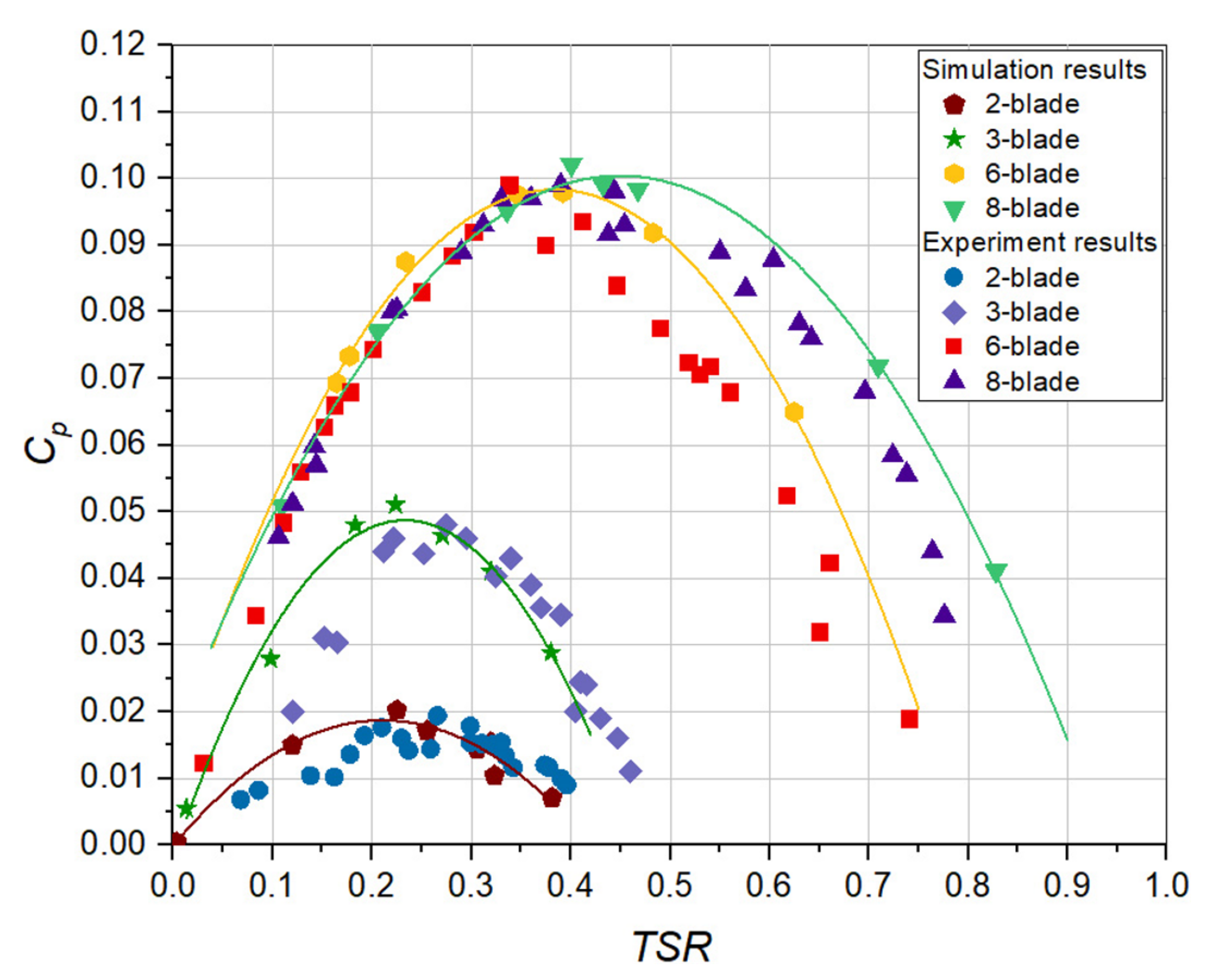
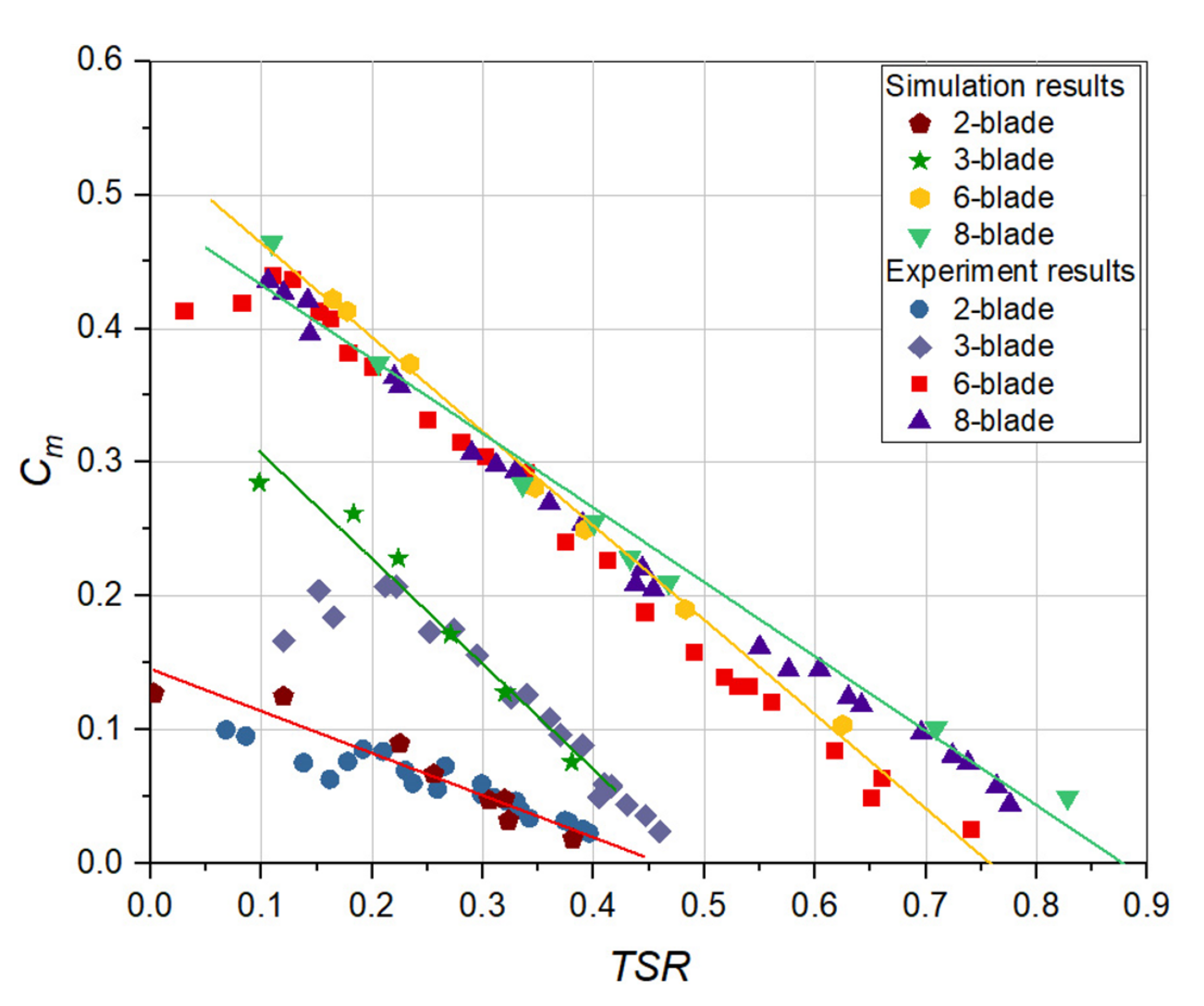
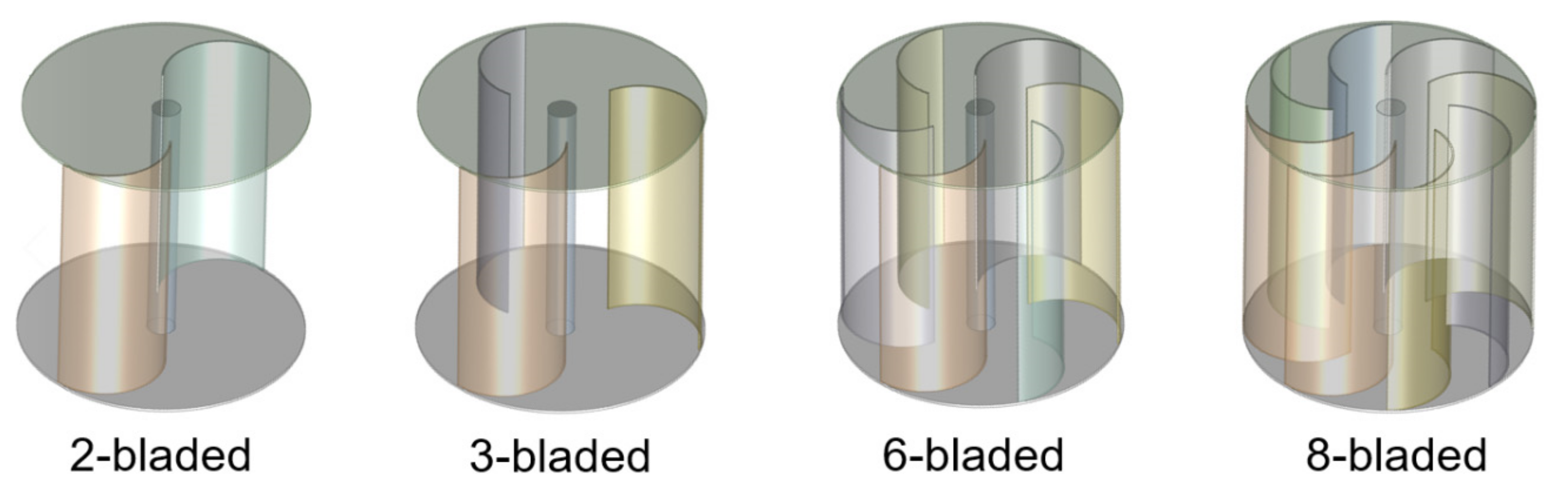
5.3. Validation and Effect of the Number of Blades

To understand the dynamics of water flow, CFD simulations were carried out to capture the variations in the water flow and rotation of the turbine. Because the number of turbine blades affects the rotational speed and torque of the turbine, simulations were carried out to investigate the effect of the number of blades. According to the results discussed in the previous chapters, the power differences among two, three, six, and eight bladed turbines with $\alpha$ = 0° and $\psi$ = 135° were simulated in the study when the inlet velocity was 1 m/s, and the results were compared with the experimental values, as shown in Figure 12. It can be observed that the simulation results had the same trend as that of the experimental results but with minor deviation and the overall characteristic curve obtain from simulations is a bit to the right of the experimental results. In the experiments, frictional drag is generated when the turbine rotates, so the angular velocity of the turbine is slower than that in the simulations. Both the experimental and simulation results showed that a greater number of blades led to a wider range of turbine speeds and greater power generation.

The performance of the six- and eight-bladed turbine was much better than that for the two- and three-bladed turbines. The maximum $C_p$ for the six-bladed turbine was 0.0979 at a TSR = 0.39, and for eight-bladed turbine, it was 0.102 at a TSR = 0.4. When the number of blades was increased to six, the efficiency produced by the turbine appeared to reach its limit.The greater the number of blades, the greater the torque load that the overall turbine can withstand, and the turbine can also reach higher speeds. The $C_m$ range for the six-bladed turbine was below 0.55; the TSR range was within 0.75; the $C_m$ range for the eight-bladed was slightly less than 0.5; and the TSR range was within 0.9. As shown in Figure 13, when the turbine speed was faster, the torque generated by the turbine was small. The $C_m$ and the TSR exhibited a linearly decreasing relationship. It can be seen that the TSR and $C_m$ values of the six-bladed turbine were very close to those for the eight-bladed distribution, which means that the two can produce similar speed ranges and torques.

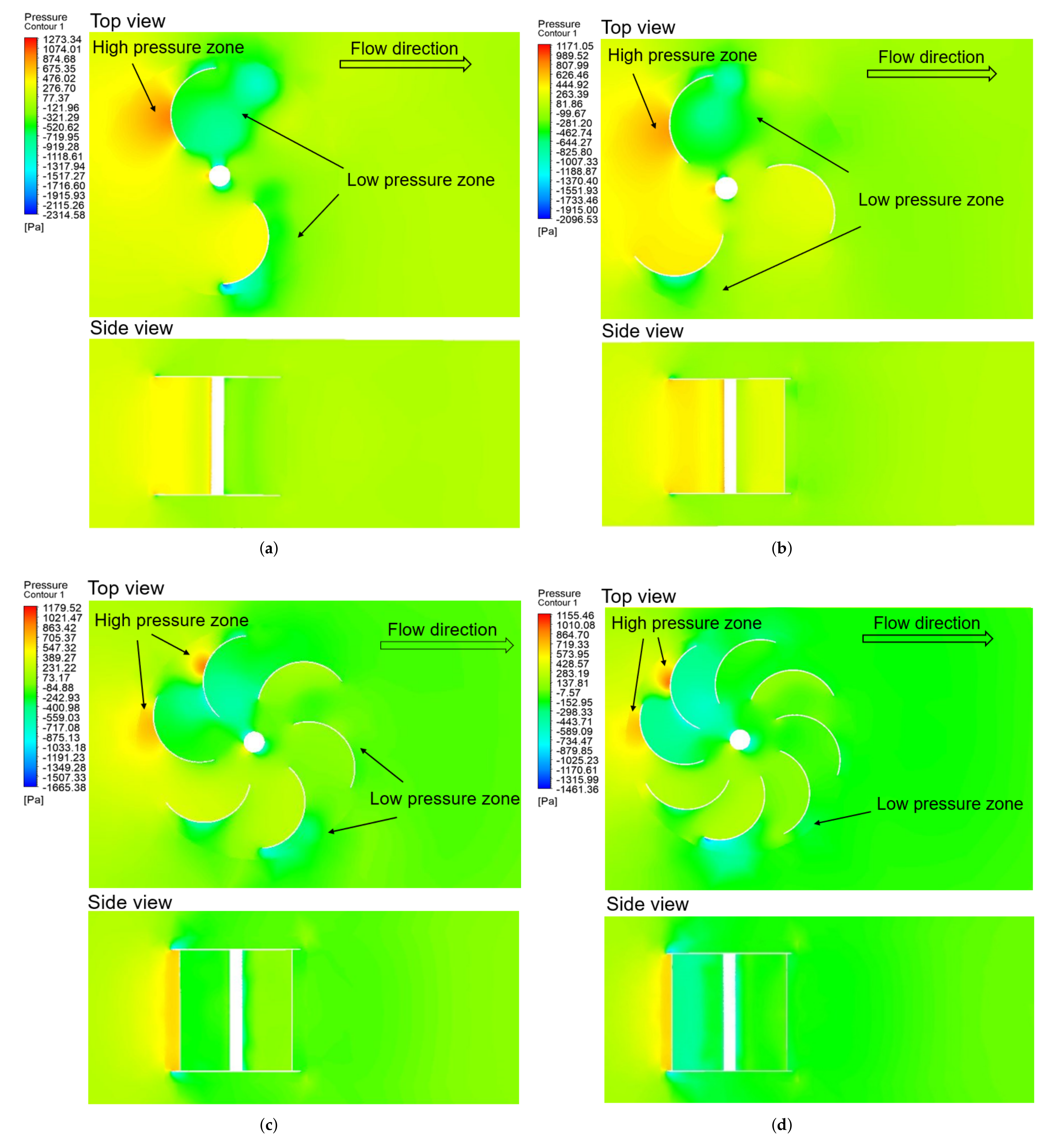
5.4. Pressure Contours

Figure 14 shows the distribution of the pressure contours among the two, three, six, and eight-bladed turbines at TSR values corresponding to the maximum power coefficient. It was observed that a pressure drop through the turbine occurred from upstream to downstream. The blades were driven to rotate because the concave surface pressure of the forward blade was greater than that of the convex surface. The eight-bladed turbine produced more positive torque due to a greater number of advancing blades, but at the same time, there were also more returning blades that provided negative torque, so the output power compared to the six-bladed reached convergence. However, its output power was still much higher than that of the two- and three-bladed turbines, which was determined by comparing the pressure difference between the upstream and downstream of the turbine. It was also observed that the high pressure zone on the convex surface of the returning blade decreased with increases in the number of blades, which reduced the amount of negative torque generated, and also indicated the consistency between the results for the simulation and the experiment. Based on the CFD simulation results, it was observed that increasing the pressure area on the concave surface of the advancing blade and reduced the pressure distribution on the convex surface of the returning blade affected by the impact of the water flow, which was the key to improve the performance of the turbine.

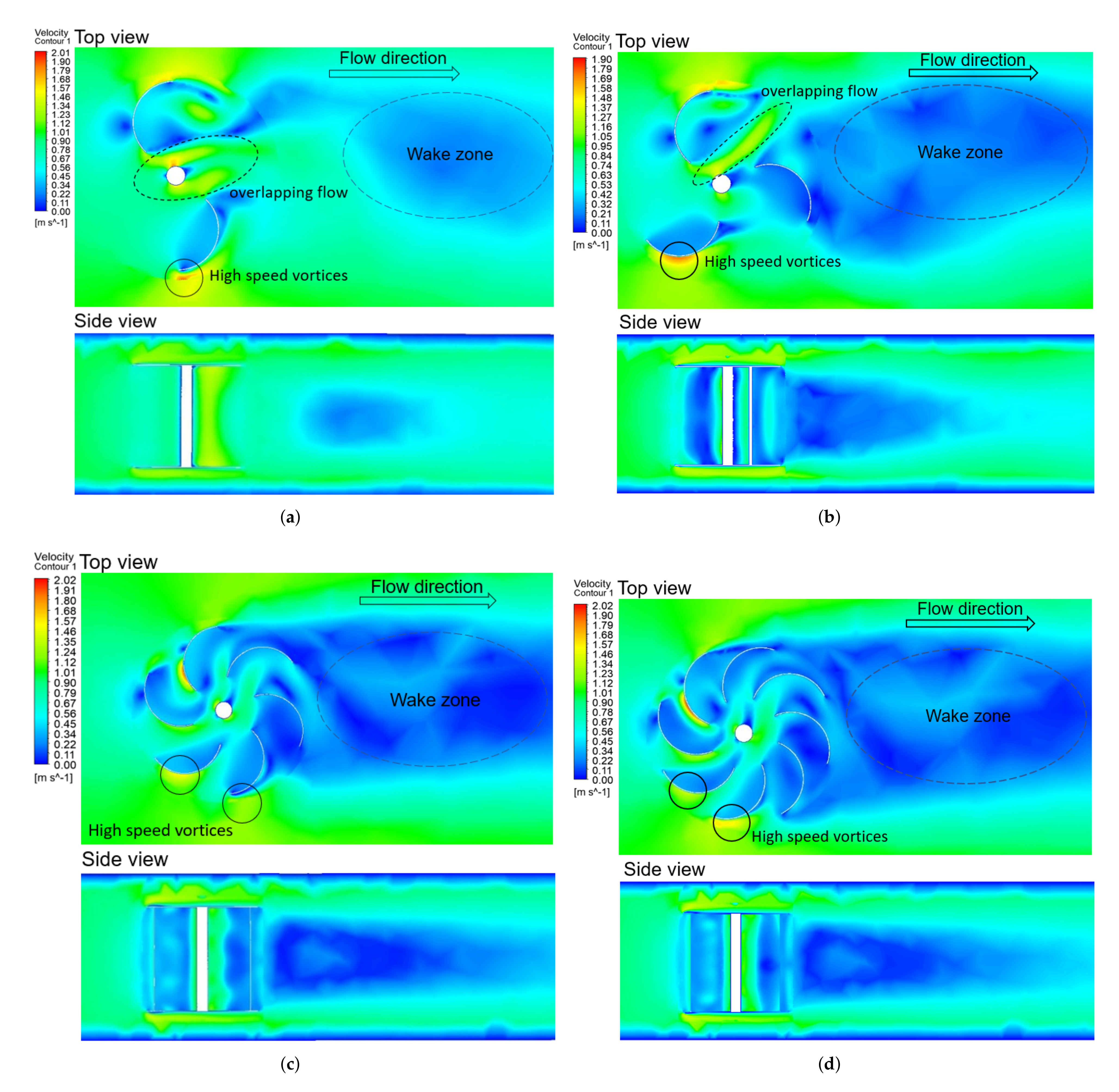
5.5. Velocity Contours

Figure 15 presents the distribution of the velocity contours among the two, three, six, and eight-bladed turbines at a TSR corresponding to the maximum power coefficient. The velocity of the water flow was constant before entering the turbine rotating domain. When the turbine rotated, it was observed that there was a high-velocity area at the tip of the advancing blade. On the other hand, a wake zone was generated downstream of the turbine. It is worth noting that the advancing blade tip of the two-bladed turbine had a more intense velocity flowing from the tip of the blade than was the case for the other turbines with more blades. This phenomenon led to a negative impact on the blade–fluid interactions, which deteriorated the efficiency of the turbine [15]. A higher velocity zone was observed at the top and bottom side, as shown in side view near the end plate. It can be observed that as the number of blades increased, this phenomenon decreased significantly, in turn improving the efficiency performance. Moreover, the overlapping flow, which can enhance the torque of the turbine, was observed to be strong on the concave surfaces of the returning blades in the case of the six- and eight-bladed turbines. However, for the eight-bladed turbine, the overlapping flow increased the hydraulic resistance of the turbine without sufficient hydrokinetic energy to impact the blades, so the performance of the six- and eight-bladed turbines was about the same. On the other hand, it was observed that the overlapping flow in the two- and three-bladed turbine left the turbine without impacting the other blades and passed through the turbine downstream. This produced vortices on the concave surfaces of the returning blade and caused a decline in the performance of the turbine.

6. Conclusions

The purpose of the current study was to investigate the influence of the blade arc angles, blade placement angle, and the number of blades on the Savonius-type hydrokinetic performance of a turbine. Considering various design parameters, the turbines were investigated and tested in an open towing tank at V = 1 m/s. Further, three-dimensional CFD simulations were performed to capture the variations in the flow field and the rotation of the turbine, which were in good agreement with the experimental results. The measured data was expressed as a dimensionless coefficient to evaluate the performance of the turbine. Moreover, the study is considered as the calibration of the CFD model for further tests and providing experiments that are difficult to be carried out. The main conclusions drawn from this study are summarized below:

• The six-bladed SHT with $\psi$ = 135° and $\alpha$ = 0° produced the highest $C_{pmax}$ of 0.099 at a TSR of 0.34.
• The performance of the blade angle of 135° was approximately 2.96 times better than the turbine of the blade angle of 180°.
• Compared with the design of the blade placement position for the reverse rotation, the forward rotation of the blade placement had less influence on the efficiency of the turbine.
• The $C_p$ and the TSR showed a quadratic curve relationship, and the $C_m$ and the TSR showed a linearly decreasing relationship.
• Based on the simulation results and the experimental results, it was found that the range of the rotational speed of the turbine became wider by increasing the number of blades due to the fact that they could harvest more hydrokinetic energy. However, when the number of blades was increased to eight, the mechanical power of the turbine reached its limit due to hydraulic resistance.
• Compared with the other turbines with varying numbers of blades, the six-bladed turbine had fewer high-speed vortices on advancing blades and more overlapping flow collisions with the returning blades. Thus, the six-bladed turbine converted more available hydro energy to the mechanical power.

In the present study, a turbine was tested at a fixed AR and water velocity in both experiments and simulations. In order to improve the performance of a turbine, it is necessary to investigate a variety of AR values, Reynolds numbers, and other design parameters to find the optimum design. There are divergent opinions on the performance of the number of SWTs in the previous literature, but in the case of the SHT, this study clearly points out that the hydrokinetic performance of the SHT increases with an increase in the number of blades, while the performance of the eight-bladed turbine reached convergence.

References

1. VanZwieten, J.; McAnally, W.; Ahmad, J.; Davis, T.; Martin, J.; Bevelhimer, M.; Cribbs, A.; Lippert, R.; Hudon, T.; Trudeau, M. In-stream hydrokinetic power: Review and appraisal. J. Energy Eng. 2015, 141, 04014024. [Google Scholar] [CrossRef]
2. Kosai, S. Dynamic vulnerability in standalone hybrid renewable energy system. Energy Convers. Manag. 2019, 180, 258–268. [Google Scholar] [CrossRef]
3. Hdom, H.A. Examining carbon dioxide emissions, fossil & renewable electricity generation and economic growth: Evidence from a panel of South American countries. Renew. Energy 2019, 139, 186–197. [Google Scholar]
4. Peng, Z.; Guo, W. Saturation characteristics for stability of hydro-turbine governing system with surge tank. Renew. Energy 2019, 131, 318–332. [Google Scholar] [CrossRef]
5. Rostami, R.; Khoshnava, S.M.; Lamit, H.; Streimikiene, D.; Mardani, A. An overview of Afghanistan’s trends toward renewable and sustainable energies. Renew. Sustain. Energy Rev. 2017, 76, 1440–1464. [Google Scholar] [CrossRef]
6. Kougias, I.; Aggidis, G.; Avellan, F.; Deniz, S.; Lundin, U.; Moro, A.; Muntean, S.; Novara, D.; Pérez-Díaz, J.I.; Quaranta, E.; et al. Analysis of emerging technologies in the hydropower sector. Renew. Sustain. Energy Rev. 2019, 113, 109257. [Google Scholar] [CrossRef]
7. Amponsah, N.Y.; Troldborg, M.; Kington, B.; Aalders, I.; Hough, R.L. Greenhouse gas emissions from renewable energy sources: A review of lifecycle considerations. Renew. Sustain. Energy Rev. 2014, 39, 461–475. [Google Scholar] [CrossRef]
8. Rostami, A.B.; Armandei, M. Renewable energy harvesting by vortex-induced motions: Review and benchmarking of technologies. Renew. Sustain. Energy Rev. 2017, 70, 193–214. [Google Scholar] [CrossRef]
9. Kumar, D.; Sarkar, S. A review on the technology, performance, design optimization, reliability, techno-economics and environmental impacts of hydrokinetic energy conversion systems. Renew. Sustain. Energy Rev. 2016, 58, 796–813. [Google Scholar] [CrossRef]
10. Khan, M.; Bhuyan, G.; Iqbal, M.; Quaicoe, J. Hydrokinetic energy conversion systems and assessment of horizontal and vertical axis turbines for river and tidal applications: A technology status review. Appl. Energy 2009, 86, 1823–1835. [Google Scholar] [CrossRef]
11. Rourke, F.O.; Boyle, F.; Reynolds, A. Marine current energy devices: Current status and possible future applications in Ireland. Renew. Sustain. Energy Rev. 2010, 14, 1026–1036. [Google Scholar] [CrossRef] [Green Version]
12. Golecha, K.; Eldho, T.; Prabhu, S. Influence of the deflector plate on the performance of modified Savonius water turbine. Appl. Energy 2011, 88, 3207–3217. [Google Scholar] [CrossRef]
13. Chen, L.; Chen, J.; Zhang, Z. Review of the Savonius rotor’s blade profile and its performance. J. Renew. Sustain. Energy 2018, 10, 013306. [Google Scholar] [CrossRef]
14. Fleming, P.; Probert, S.; Tanton, D. Designs and performances of flexible and taut sail Savonius-type wind-turbines. Appl. Energy 1985, 19, 97–110. [Google Scholar] [CrossRef]
15. Sarma, N.; Biswas, A.; Misra, R. Experimental and computational evaluation of Savonius hydrokinetic turbine for low velocity condition with comparison to Savonius wind turbine at the same input power. Energy Convers. Manag. 2014, 83, 88–98. [Google Scholar] [CrossRef]
16. Chen, B.; Nagata, S.; Murakami, T.; Ning, D. Improvement of sinusoidal pitch for vertical-axis hydrokinetic turbines and influence of rotational inertia. Ocean. Eng. 2019, 179, 273–284. [Google Scholar] [CrossRef]
17. Gorelov, D.; Krivospitsky, V. Prospects for development of wind turbines with orthogonal rotor. Thermophys. Aeromech. 2008, 15, 153–157. [Google Scholar] [CrossRef]
18. Patel, V.; Eldho, T.; Prabhu, S. Theoretical study on the prediction of the hydrodynamic performance of a Savonius turbine based on stagnation pressure and impulse momentum principle. Energy Convers. Manag. 2018, 168, 545–563. [Google Scholar] [CrossRef]
19. Blackwell, B.F.; Feltz, L.V.; Sheldahl, R.E. Wind Tunnel Performance Data for Two- and Three-Bucket Savonius Rotors; Sandia Laboratories Albuquerque: Albuquerque, NM, USA, 1977. [Google Scholar]
20. Sivasegaram, S. Secondary parameters affecting the performance of resistance-type vertical-axis wind rotors. Wind Eng. 1978, 2, 49–58. [Google Scholar]
21. Khan, M.H. Model and prototype performance characteristics of Savonius rotor windmill. Wind Eng. 1978, 2, 75–85. [Google Scholar]
22. Ushiyama, I.; Nagai, H. Optimum design configurations and performance of Savonius rotors. Wind Eng. 1988, 12, 59–75. [Google Scholar]
23. Fujisawa, N.; Gotoh, F. Experimental study on the aerodynamic performance of a Savonius rotor. J. Sol. Energy Eng. 1994, 116, 148–152. [Google Scholar] [CrossRef]
24. Sheldahl, R.E.; Blackwell, B.F.; Feltz, L.V. Wind tunnel performance data for two-and three-bucket Savonius rotors. J. Energy 1978, 2, 160–164. [Google Scholar] [CrossRef] [Green Version]
25. Emmanuel, B.; Jun, W. Numerical study of a six-bladed Savonius wind turbine. J. Sol. Energy Eng. 2011, 133, 044503. [Google Scholar] [CrossRef]
26. Mahmoud, N.; El-Haroun, A.; Wahba, E.; Nasef, M. An experimental study on improvement of Savonius rotor performance. Alex. Eng. J. 2012, 51, 19–25. [Google Scholar] [CrossRef] [Green Version]
27. Wenehenubun, F.; Saputra, A.; Sutanto, H. An experimental study on the performance of Savonius wind turbines related with the number of blades. Energy Procedia 2015, 68, 297–304. [Google Scholar] [CrossRef] [Green Version]
28. Banerjee, A.; Roy, S.; Mukherjee, P.; Saha, U.K. Unsteady flow analysis around an elliptic-bladed Savonius-style wind turbine. In Proceedings of the Gas Turbine India Conference, New Delhi, India, 15–17 December 2014; American Society of Mechanical Engineers: New York, NY, USA, 2014; Volume 49644, p. V001T05A001. [Google Scholar]
29. Alom, N.; Kolaparthi, S.C.; Gadde, S.C.; Saha, U.K. Aerodynamic design optimization of elliptical-bladed Savonius-Style wind turbine by numerical simulations. In Proceedings of the International Conference on Offshore Mechanics and Arctic Engineering, Busan, Korea, 19–24 June 2016; American Society of Mechanical Engineers: New York, NY, USA, 2016; Volume 49972, p. V006T09A009. [Google Scholar]
30. Abdelaziz, K.R.; Nawar, M.A.; Ramadan, A.; Attai, Y.A.; Mohamed, M.H. Performance improvement of a Savonius turbine by using auxiliary blades. Energy 2021, 244, 122575. [Google Scholar] [CrossRef]
31. Faizal, M.; Ahmed, M.R.; Lee, Y.H. On utilizing the orbital motion in water waves to drive a Savonius rotor. Renew. Energy 2010, 35, 164–169. [Google Scholar] [CrossRef]
32. Yaakob, O.; Ahmed, Y.M.; Ismail, M.A. Validation study for Savonius vertical axis marine current turbine using CFD simulation. In Proceedings of the 6th Asia-Pacific Workshop on Marine Hydrodynamics-APHydro2012, Johor Bahru, Malaysia, 3–4 September 2012; pp. 3–4. [Google Scholar]
33. Khan, M.; Islam, N.; Iqbal, T.; Hinchey, M.; Masek, V. Performance of Savonius rotor as a water current turbine. J. Ocean. Technol. 2009, 4, 71–83. [Google Scholar]
34. Kailash, G.; Eldho, T.; Prabhu, S. Performance study of modified Savonius water turbine with two deflector plates. Int. J. Rotating Mach. 2012, 2012, 679247. [Google Scholar] [CrossRef] [Green Version]
35. Patel, V.; Bhat, G.; Eldho, T.; Prabhu, S. Influence of overlap ratio and aspect ratio on the performance of Savonius hydrokinetic turbine. Int. J. Energy Res. 2017, 41, 829–844. [Google Scholar] [CrossRef]
36. Kumar, A.; Saini, R. Performance analysis of a Savonius hydrokinetic turbine having twisted blades. Renew. Energy 2017, 108, 502–522. [Google Scholar] [CrossRef]
37. Talukdar, P.K.; Sardar, A.; Kulkarni, V.; Saha, U.K. Parametric analysis of model Savonius hydrokinetic turbines through experimental and computational investigations. Energy Convers. Manag. 2018, 158, 36–49. [Google Scholar] [CrossRef]
38. Mosbahi, M.; Ayadi, A.; Chouaibi, Y.; Driss, Z.; Tucciarelli, T. Performance study of a Helical Savonius hydrokinetic turbine with a new deflector system design. Energy Convers. Manag. 2019, 194, 55–74. [Google Scholar] [CrossRef]
39. Guo, F.; Song, B.; Mao, Z.; Tian, W. Experimental and numerical validation of the influence on Savonius turbine caused by rear deflector. Energy 2020, 196, 117132. [Google Scholar] [CrossRef]
40. Zhao, Z.; Zheng, Y.; Xu, X.; Liu, W.; Hu, G. Research on the improvement of the performance of Savonius rotor based on numerical study. In Proceedings of the 2009 International Conference on Sustainable Power Generation and Supply, Nanjing, China, 6–7 April 2009; pp. 1–6. [Google Scholar]
41. Ragheb, M.; Ragheb, A.M. Wind turbines theory-the betz equation and optimal rotor tip speed ratio. Fundam. Adv. Top. Wind. Power 2011, 1, 19–38. [Google Scholar]
42. Alexander, A.; Holownia, B. Wind tunnel tests on a Savonius rotor. J. Wind. Eng. Ind. Aerodyn. 1978, 3, 343–351. [Google Scholar] [CrossRef]
43. Yao, J.; Li, F.; Chen, J.; Yuan, Z.; Mai, W. Parameter analysis of Savonius hydraulic turbine considering the effect of reducing flow velocity. Energies 2019, 13, 24. [Google Scholar] [CrossRef] [Green Version]
44. Tian, W.; Mao, Z.; Zhang, B.; Li, Y. Shape optimization of a Savonius wind rotor with different convex and concave sides. Renew. Energy 2018, 117, 287–299. [Google Scholar] [CrossRef]
45. Kacprzak, K.; Liskiewicz, G.; Sobczak, K. Numerical investigation of conventional and modified Savonius wind turbines. Renew. Energy 2013, 60, 578–585. [Google Scholar] [CrossRef]
46. Mohamed, M.; Janiga, G.; Pap, E.; Thévenin, D. Optimal blade shape of a modified Savonius turbine using an obstacle shielding the returning blade. Energy Convers. Manag. 2011, 52, 236–242. [Google Scholar] [CrossRef]
47. Mari, M.; Venturini, M.; Beyene, A. A novel geometry for vertical axis wind turbines based on the Savonius concept. J. Energy Resour. Technol. 2017, 139, 061202. [Google Scholar] [CrossRef]
48. Versteeg, H.K.; Malalasekera, W. An Introduction to Computational Fluid Dynamics: The Finite Volume Method; Pearson Education: London, UK, 2007. [Google Scholar]
49. Succi, S.; Pappetti, F.; Succi, S. An Introduction to Parallel Computational Fluid Dynamics; Nova Publishers: Hauppauge, NY, USA, 1996. [Google Scholar]
50. Wahyudi, B.; Soeparman, S.; Wahyudi, S.; Denny, W. A simulation study of Flow and Pressure distribution patterns in and around of Tandem Blade Rotor of Savonius (TBS) Hydrokinetic turbine model. J. Clean Energy Technol. 2013, 1, 286–291. [Google Scholar] [CrossRef] [Green Version]
51. Driss, Z.; Jemni, M.; Chelly, A.; Abid, M. Computational study of a vertical axis water turbine placed in a hydrodynamic test bench. Int. J. Mech. Appl. 2013, 3, 98–104. [Google Scholar]
52. Roy, S.; Saha, U.K. Computational study to assess the influence of overlap ratio on static torque characteristics of a vertical axis wind turbine. Procedia Eng. 2013, 51, 694–702. [Google Scholar] [CrossRef] [Green Version]
53. Roy, S.; Saha, U.K. Wind tunnel experiments of a newly developed two-bladed Savonius-style wind turbine. Appl. Energy 2015, 137, 117–125. [Google Scholar] [CrossRef]
54. Mao, Z.; Tian, W. Effect of the blade arc angle on the performance of a Savonius wind turbine. Adv. Mech. Eng. 2015, 7, 1687814015584247. [Google Scholar] [CrossRef]
Figure 1. Schematic diagram of a 6-bladed turbine.
Energies 15 01856 g001
Figure 2. The geometry of the turbine blades with different arc angles ( ψ = 135° and 180°).
Energies 15 01856 g002
Figure 3. The geometry of the turbine blades at different placement angles ( α = ±22.5°).
Energies 15 01856 g003
Figure 4. The geometry of the turbine for different numbers of blades ( α = 0°, ψ = 135°).
Energies 15 01856 g004
Figure 5. Schematic diagram of the towing tank.
Energies 15 01856 g005
Figure 6. Towing tank experimental platform.
Energies 15 01856 g006
Figure 7. Rotation of the 6-bladed turbine in the tank.
Energies 15 01856 g007
Figure 8. Dimensions of the flow field.
Energies 15 01856 g008
Figure 9. Computational domain mesh details (prism mesh).
Energies 15 01856 g009
Figure 10. Variation in C m and C p with the TSR for the different blade arc angles ( ψ ). (a) C m vs. TSR, (b) C p vs. TSR.
Energies 15 01856 g010
Figure 11. Variation in C m and C p with the TSR for the different blade placement angles ( α ). (a) C m vs. TSR, (b) C p vs. TSR.
Energies 15 01856 g011
Figure 12. Effect of the number of blades on the power coefficient for different TSR values (experimental and simulation results).
Energies 15 01856 g012
Figure 13. Effect of the number of blades on the moment coefficient for different TSR values (experimental and simulation results).
Energies 15 01856 g013
Figure 14. Comparison of the pressure distribution around the blades for (a) 2-bladed turbine, (b) 3-bladed turbine, (c) 6-bladed turbine, and (d) 8-bladed turbine.
Energies 15 01856 g014
Figure 15. Comparison of the velocity distribution around the blades for (a) 2-bladed turbine, (b) 3-bladed turbine, (c) 6-bladed turbine, and (d) 8-bladed turbine.
Energies 15 01856 g015