
Artificial Neural Network Based Optimal Feedforward Torque Control of Interior Permanent Magnet Synchronous Machines: A Feasibility Study and Comparison with the State-of-the-Art


Abstract
:Notation
1. Introduction
1.1. Motivation
1.2. Detailed Literature Review
1.2.1. Optimal Feedforward Torque Control (OFTC)
1.2.2. Artificial Neural Networks in Electrical Drives
1.2.3. Summary of Detailed Literature Review
1.3. Problem Statement
1.4. Proposed Solution
2. Artificial Neural Network based Optimal Feedforward Torque Control
- The approximation accuracy of the ANN for OFTC must be (very) high, i.e., approximation errors should be smaller than ;
- Assuming the required data is available, there are no stringent restrictions on training and validation as it is performed offline, i.e., there are (almost) no computational or memory storage constraints during training and validation; and
- The trained ANN should be simple to implement and run in real-time, i.e., a rather small feedforward network architecture (i.e., without dynamics; no recurrent network) with a low number of neurons and one or (at most) two hidden layers should be used.
2.1. Artificial Neural Network Design
2.1.1. Preliminaries: Neurons, Layers and Recursive Output Computation
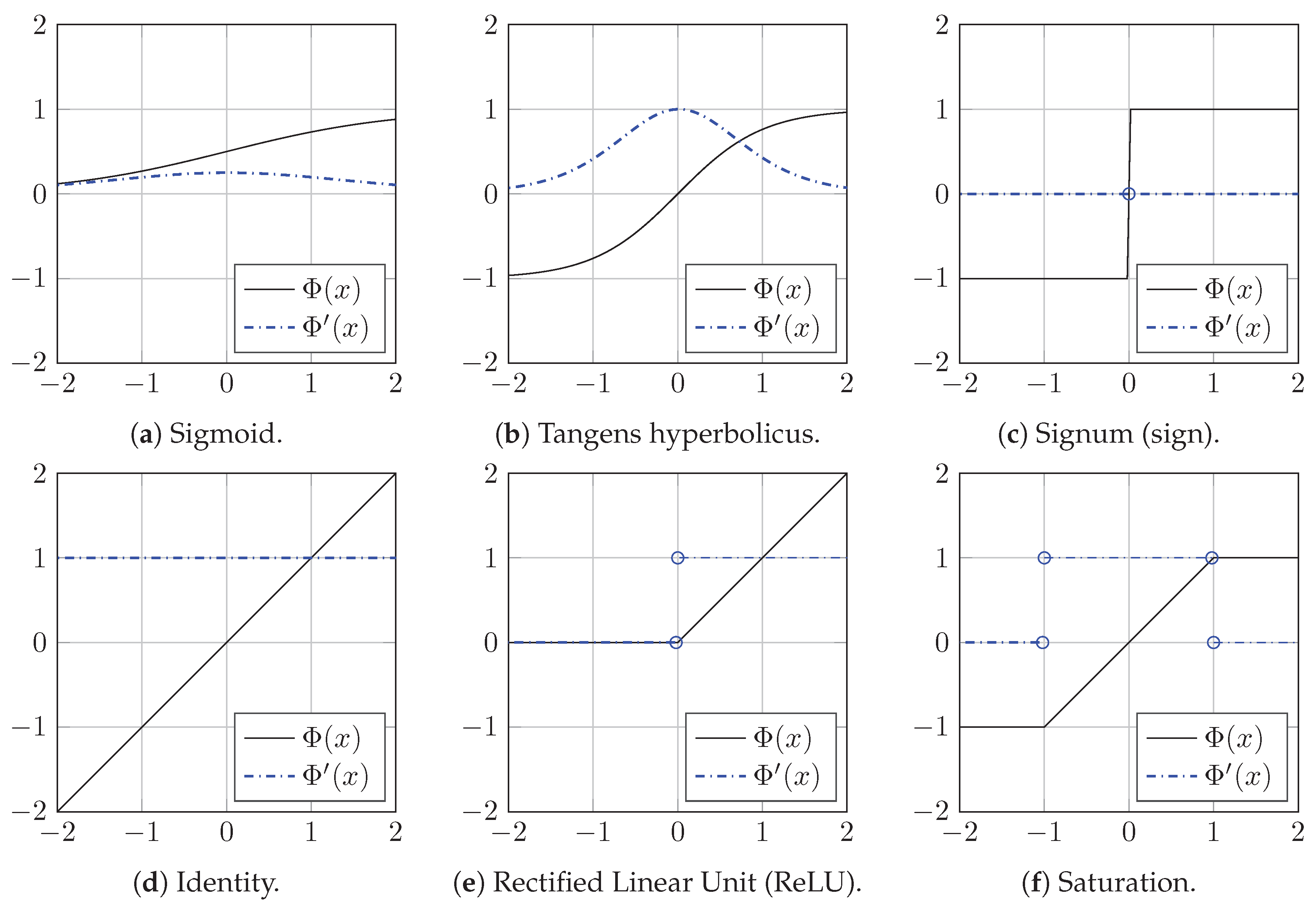
2.1.2. Activation Functions
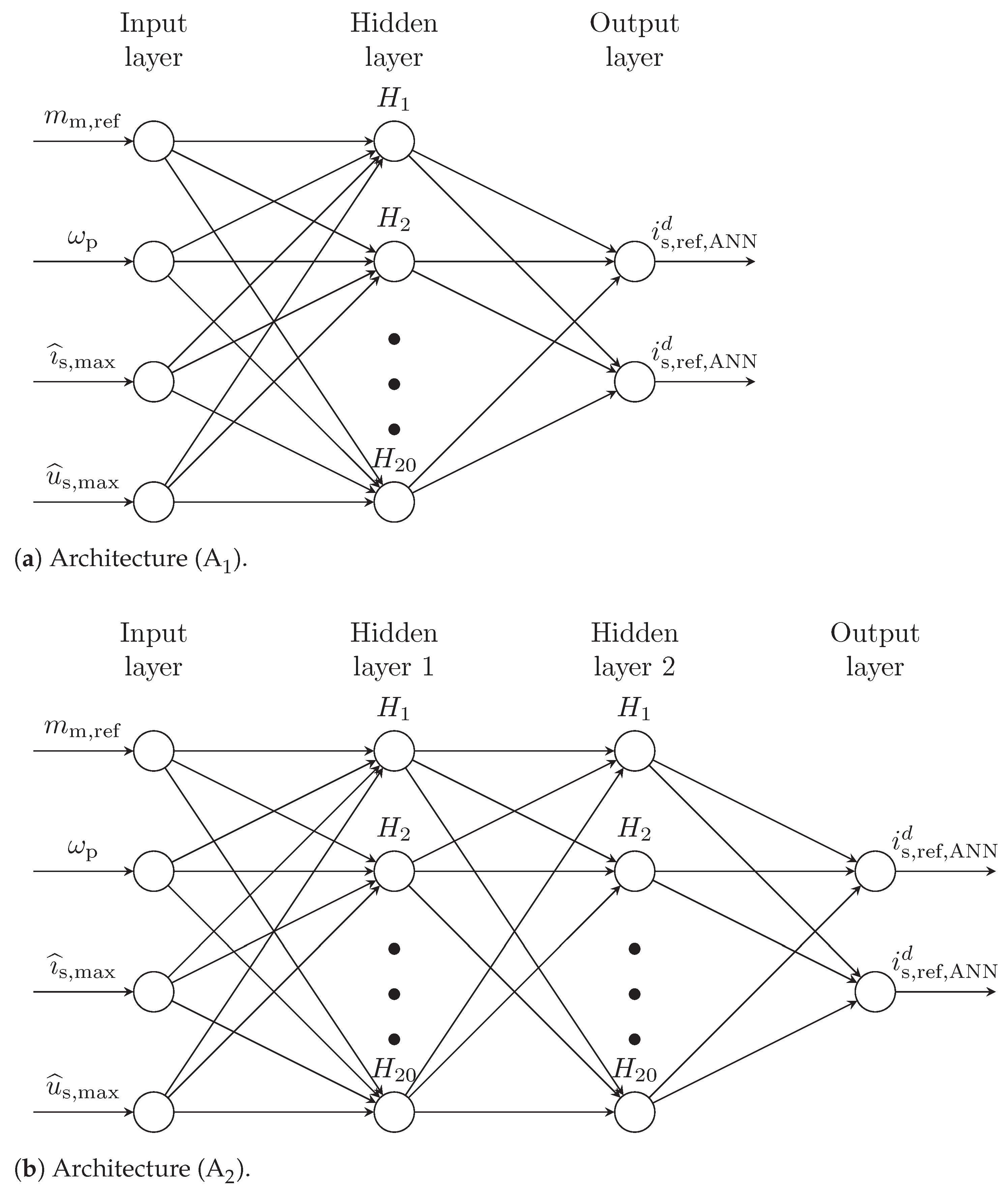
2.1.3. Implemented Artificial Neural Network Architectures
- for one hidden layer (i.e., ) and
- for two hidden layers (i.e., ).
2.2. Artificial Neural Network Training
2.2.1. Preliminaries: Data Sets, Performance Measures and Training Algorithms
- Mean Error (ME)
- Standard Error Deviation (SED)
- Quadratic Euclidean Distance (or Mean Squared Error (MSE))
- (Region I);
- (Region II); and
- (Region III);
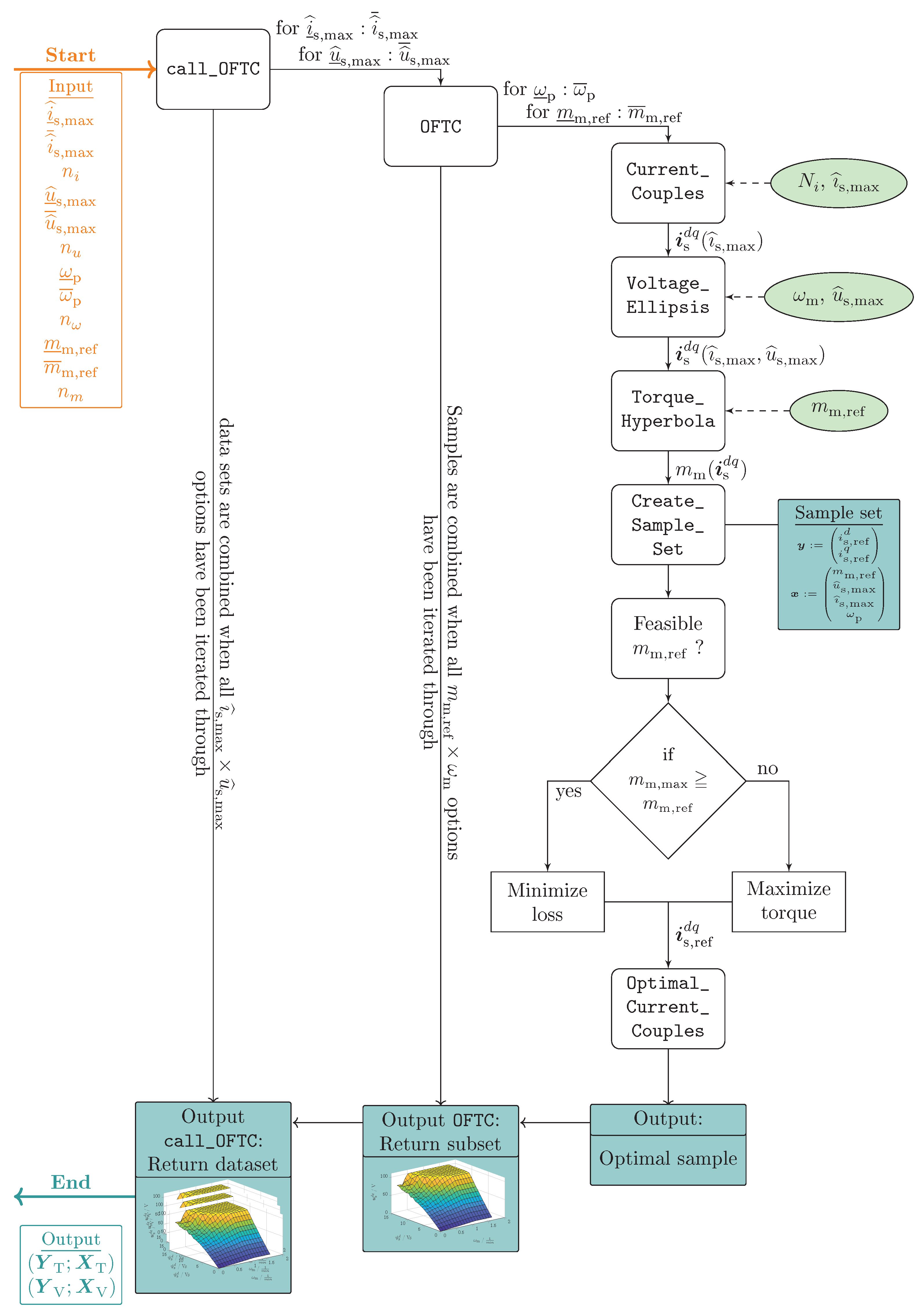
2.2.2. Data Set(s) Creation for Training (and Validation)
- the available rated machine parameters (see Table 3) such as e.g., pole pair number , resistance at rated temperature, moment of inertia , rated torque and rated current magnitude ;
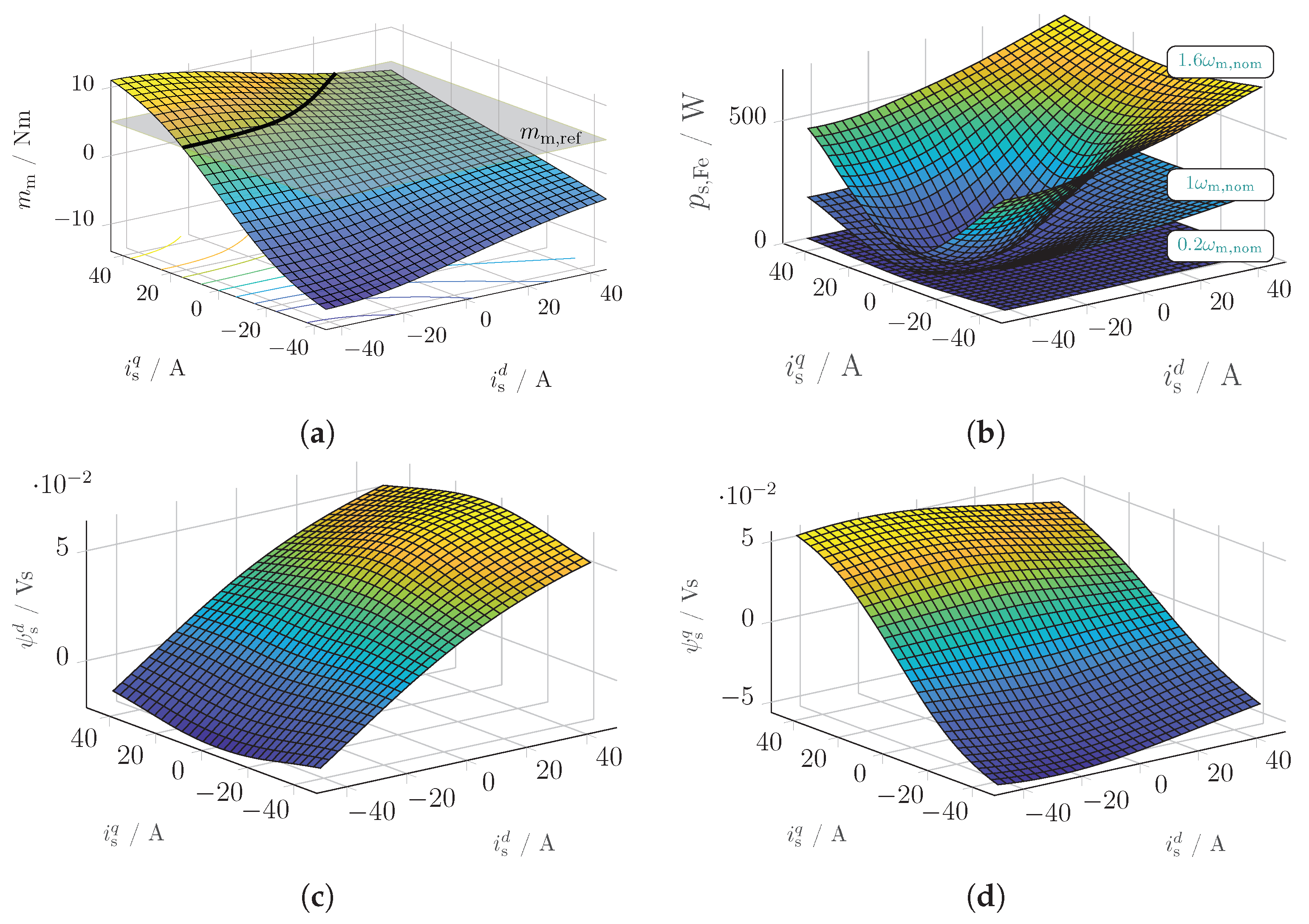
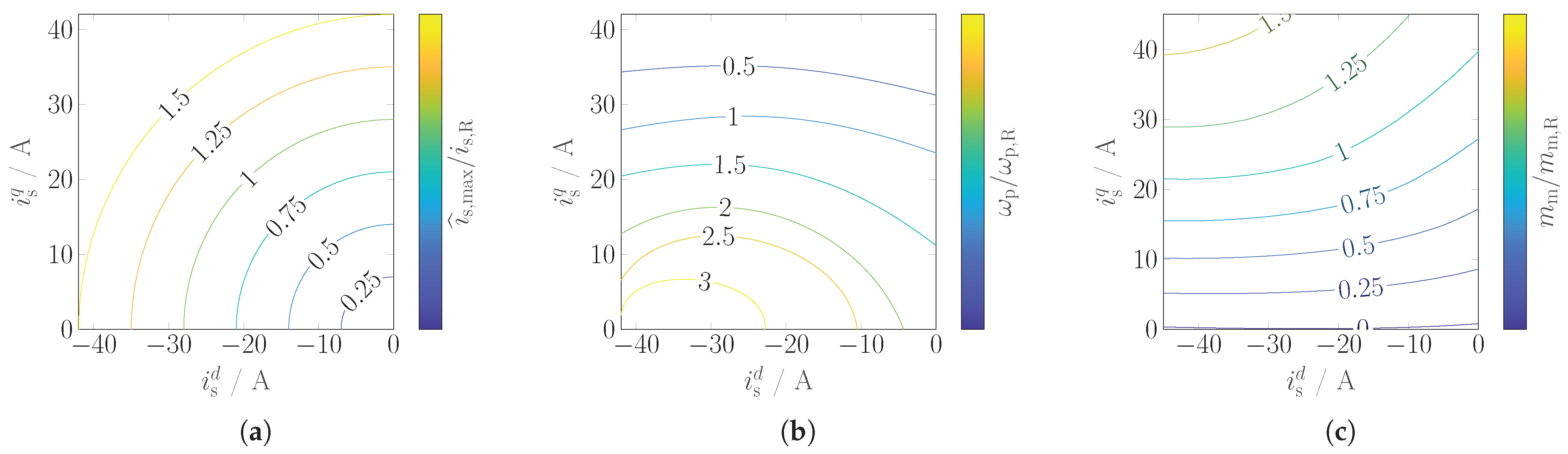
- the available LUTs for iron losses, flux linkages and machine torque parametrized by the angular velocity (or ; see Figure 4) and the -currents within the current circle
- the admissible ranges of the current and voltage limits, given bywith lower (, ) and upper (, ) bounds on these limits.

| Description | Symbol & Value | Unit |
|---|---|---|
| Rated power (mechanical) | ||
| Rated torque (mechanical) | = | |
| Rated speed (mechanical) | = 5500 ( = ) | () |
| Rated current (magnitude) | = 35 | |
| Maximal stator current (magnitude) | = 35 | |
| Maximal stator voltage (magnitude) | = 110 | |
| Stator resistance (at nominal temperature) | = | |
| Inertia | = | |
| Pole pair number | - |
2.2.3. Data Set Preprocessing for Training (and Validation)
2.2.4. Network Training
2.2.5. Avoidance of Overfitting
- proper training (and validation) sets must be chosen in order to cover all relevant regions (operating points) for ANN-based OFTC; in particular, a proper size of the training set (number of operating points) must be found. Therefore, three different sizes (small, medium and large) of training sets for training and two validation sets for validation were used and their respective results were compared. The sets have been generated by Monte Carlo simulation while an optimal coverage of the desired operating points was assured. Those sets leading to the best approximation performance of the ANN were finally used; and
- proper termination criteria for the training process must be formulated (see Table 6 and, for more details, see Chapter 11.5.2 in [66]), in particular, during training a quick parallel validation is performed and if here the validation approximation error increases for a certain number of epochs in a row (see solid green lines in Figure 15), the training is stopped and the trained weights before the increase of the approximation error are used as final weights for the trained ANN.
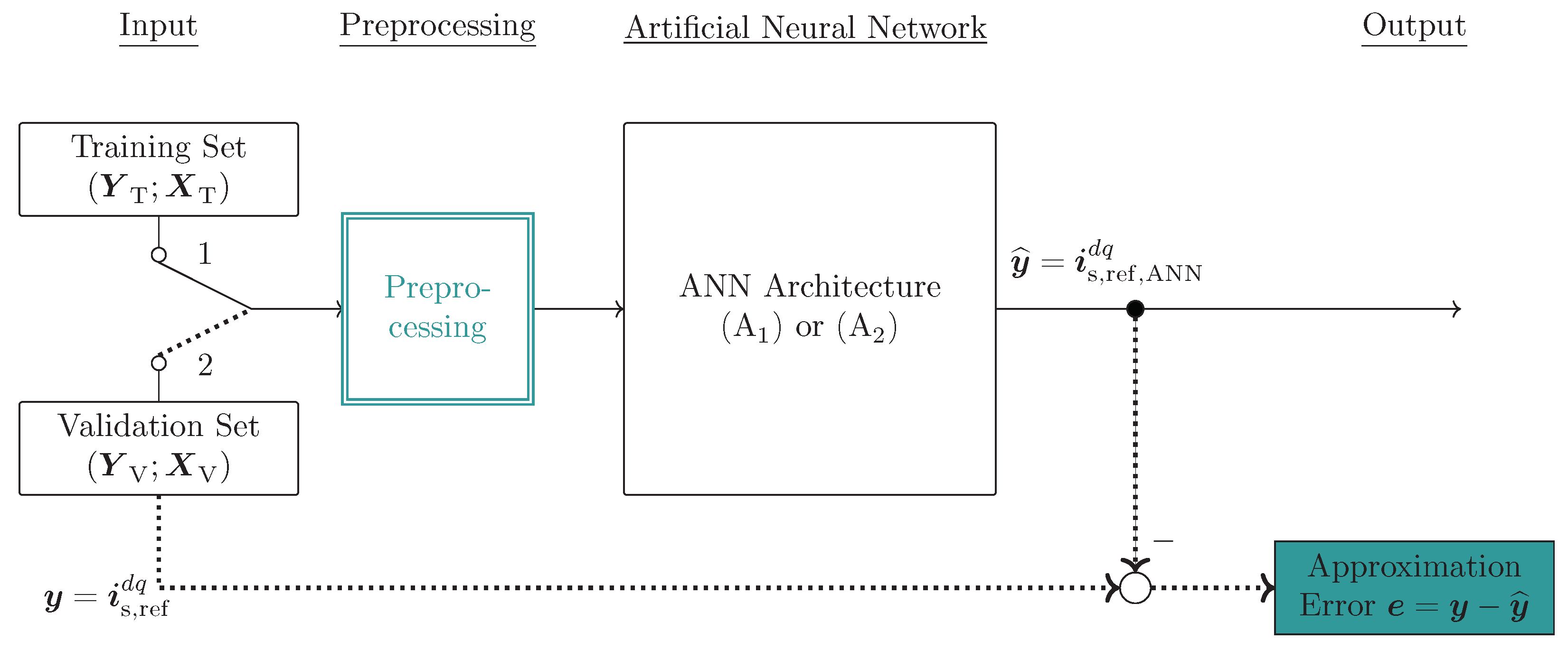
2.3. Artificial Neural Network Validation
2.3.1. Validation Procedure
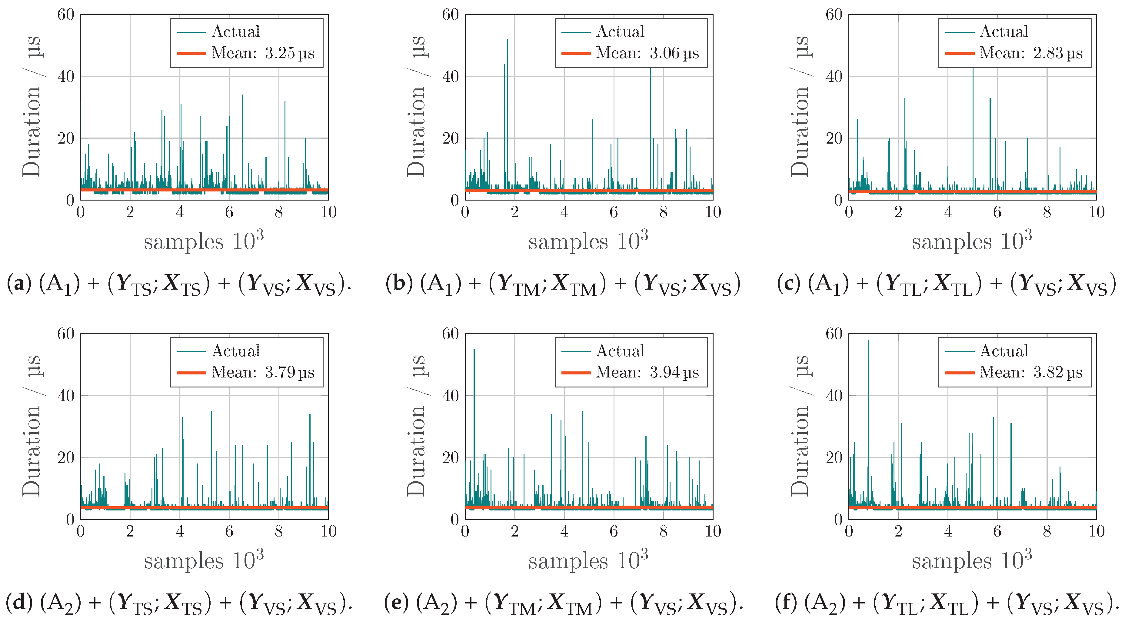
2.3.2. Validation Scenario I: Execution Time
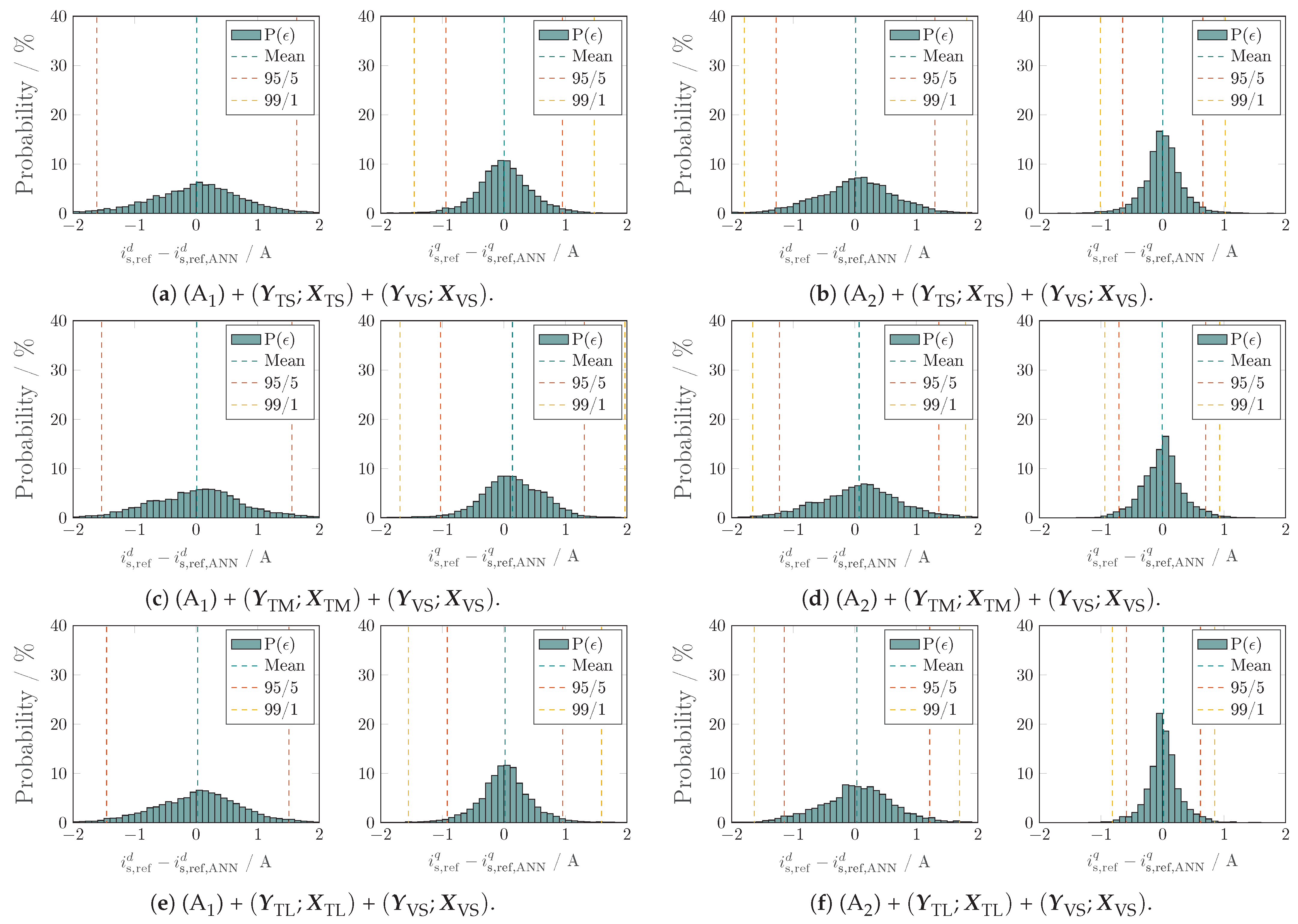
2.3.3. Validation Scenario II: Approximation Accuracy
3. Closed-Loop Implementation and Comparison
- OFTC: OFTC with ORCC using the MATLAB-function fmincon (solving the nonlinear problem (NLP) directly);
- OFTC: OFTC with ORCC using pre-generated LUTs;
- OFTC: OFTC with numerical ORCC;
- OFTC: OFTC with analytical ORCC; and
- OFTC: OFTC with ORCC utilizing the proposed ANN.
3.1. Description of Closed-Loop Implementation
3.2. Implementation Results and Discussion
 ] and reference or maximum values [
  ] of stator currents and , current magnitude , voltage magnitude , machine speed (in ) and torque are shown in Figure 19, where the left column [see Figure 19a] presents the simulation results for OFTC with analytical ORCC (OFTC) and the right column [see Figure 19b] for ANN-based OFTC (OFTC).
 ], MC [
  ], MC [
  ] and FW [
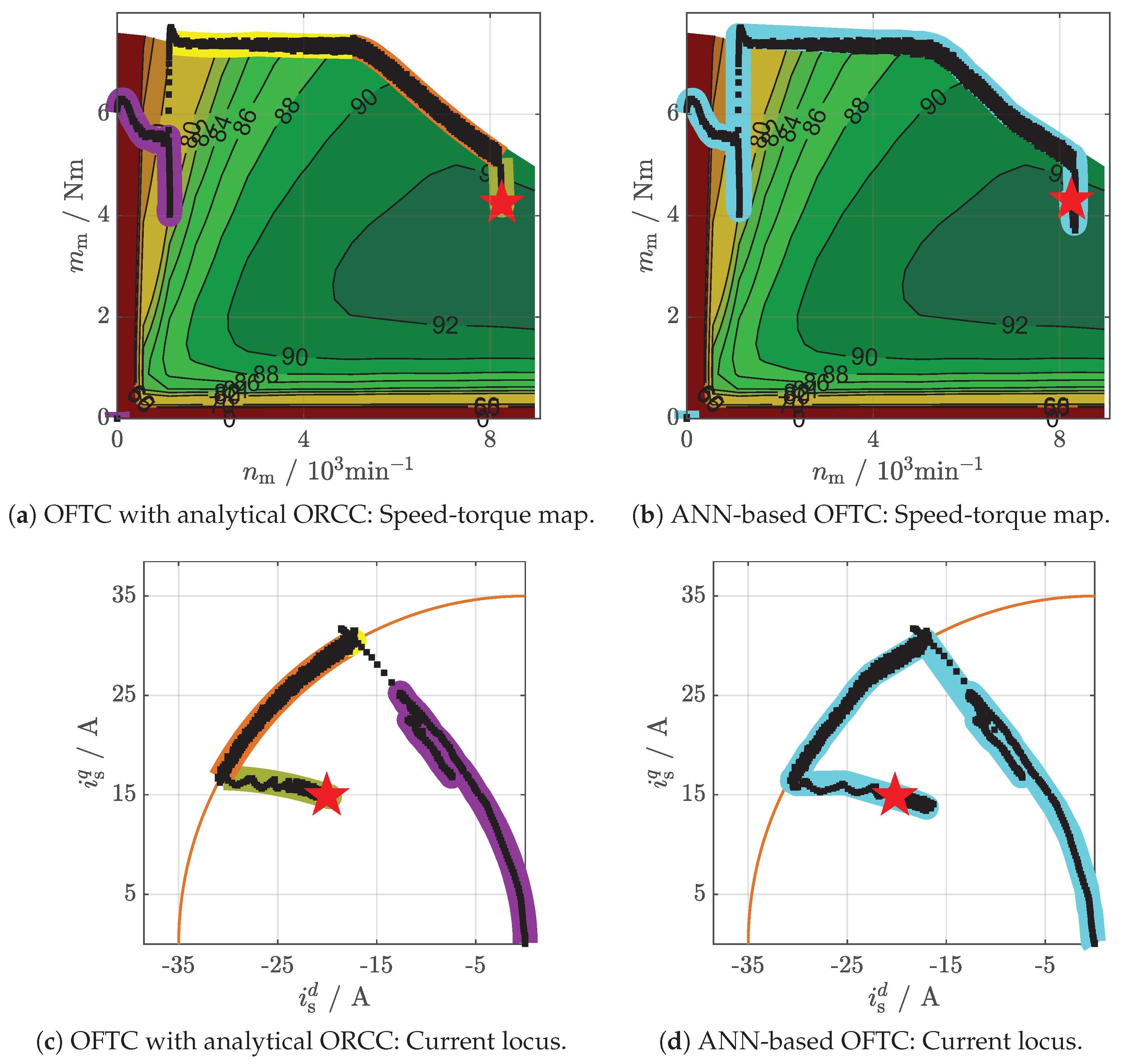
  ] (for details see [4,5,25]). Despite the fact, that the ANN-based OFTC does not distinguish between different operation strategies, the background colors from Figure 19a are used in Figure 19b as well to allow for an easier comparison.] is active until .] becomes active. The valid current couples move on the current circle to more negative reference currents [i.e., , see also current loci in Figure 20b,d, respectively]. Consequently, the produced machine torque is smaller than the reference torque, since it is not feasible anymore due to the active current and voltage constraints.]. After some transients due to the current control system, the final operating point [★] is reached at and the machine speed remains constant until the simulation ends at . The efficiency for both strategies is at its maximum for all operating conditions [cf. Figure 20a,b for OFTC with analytical ORCC and for ANN-based OFTC, respectively].], ANN-based OFTC [
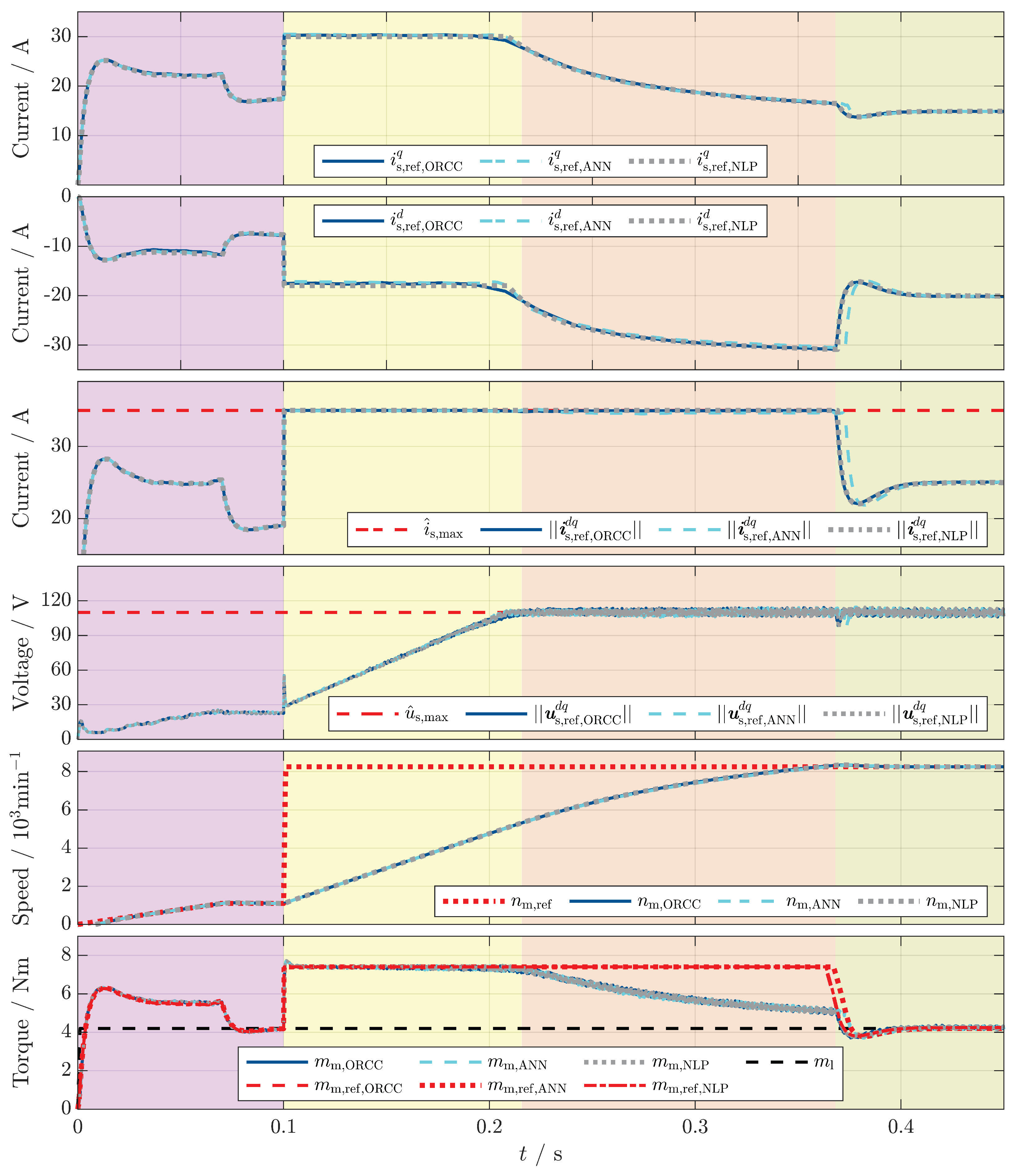
  ] are compared with the optimal reference currents and obtained by directly solving the Nonlinear Optimization Problem (NLP) problem (5) with the MATLAB function fmincon [
  ]. The NLP values are considered the benchmark values for the other two OFTC approaches. The plotted signals in Figure 21 are the actual reference currents, utilized reference current magnitude , utilized voltage magnitude , actual machine speed (in ) and actual machine torque . The results show that, in particular, all reference current pairs of OFTC with ORCC and ANN-based OFTC are very similar and close to those obtained by the OFTC solved directly by fmincon (NLP). Only very small deviations can be observed: From to , the current magnitude of ANN-based OFTC is slightly below the current limit. Therefore, the torque potential is not completely utilized to its full extent. That is why the target speed is reached about later by the ANN-based OFTC than by the other OFTC approaches.
4. Summary and Outlook
Author Contributions
Funding
Conflicts of Interest
Abbreviations
| ADALINE | Adaptive Linear Neuron |
| ANN | Artificial Neural Network |
| back-EMF | back-Electromotive Force |
| BEV | Battery Electric Vehicle |
| CNN | Convolutional Neural Network |
| DNN | Deep Neural Network |
| DSP | Digital Signal Processor |
| FE | Finite Element |
| FEA | Finite Element Analysis |
| FNN | Feedforward Neural Network |
| FLOPS | Floating Point Operations |
| FOC | Field-Oriented Control |
| FPGA | Field-Programmable Gate Array |
| FW | Field Weakening |
| HEV | Hybrid Electric Vehicle |
| IPMSM | Interior Permanent Magnet Synchronous Machine |
| IAE | Integral Absolute Error |
| LMA | Loss Minimization Algorithm |
| LMC | Loss Minimization Control |
| LSTM | Long Short-Term Memory |
| LUT | Look-Up Table |
| MC | Maximum Current |
| MCSA | Motor Current Signature Analysis |
| MLP | Multilayer Perceptron |
| MDPI | Multidisciplinary Digital Publishing Institute |
| ME | Mean Error |
| MEPA | Maximum Efficiency per Ampere |
| MPC | Model Predictive Control |
| MRAC | Model Reference Adaptive Controller |
| MSE | Mean Squared Error |
| MTPA | Maximum Torque per Ampere |
| MTPC | Maximum Torque per Current |
| MTPF | Maximum Torque per Flux |
| MTPL | Maximum Torque per Losses |
| MTPV | Maximum Torque per Voltage |
| NAN | Not A Number |
| NLP | Nonlinear Optimization Problem |
| OFTC | Optimal Feedforward Torque Control |
| OOSS | Optimal Operation Strategy Selection |
| OPP | Optimal Pulse Pattern |
| ORCC | Optimal Reference Current Computation |
| PHEV | Hybrid Electric Vehicles |
| PMSM | Permanent Magnet Synchronous Machine |
| PNN | Probabilistic Neural Network |
| PTC | Predictive Torque Controller |
| RBF | Radial Basis Function |
| ReLU | Rectified Linear Unit |
| RNG | Random Number Generator |
| RNN | Recurrent Neural Network |
| SED | Standard Error Deviation |
| SM | Synchronous Machine |
| VMC | Voltage Matching Circuit |
References
- De Almeida, A.; Ferreira, F.; Fong, J. Standards for Efficiency of Electric Motors. IEEE Ind. Appl. Mag. 2011, 17, 12–19. [Google Scholar] [CrossRef]
- Ritchie, H.; Roser, M. Energy Mix. 2021. Available online: https://ourworldindata.org/energy-mix (accessed on 28 June 2021).
- Eroglu, I.; Horlbeck, L.; Lienkamp, M.; Hackl, C. Increasing the Overall Efficiency of Induction Motors for BEV by using the Overload Potential through Downsizing. In Proceedings of the IEEE International Electric Machines & Drives Conference (IEMDC 2017), Miami, FL, USA, 21–24 May 2017. [Google Scholar]
- Hackl, C.; Kullick, J.; Monzen, N. Optimale Betriebsführung für nichtlineare Synchronmaschinen. In Elektrische Antriebe–Regelung von Antriebssystemen; Böcker, J., Griepentrog, G., Eds.; Springer: Berlin/Heidelberg, Germany, 2020. [Google Scholar]
- Hackl, C.M.; Kullick, J.; Monzen, N. Generic loss minimization for nonlinear synchronous machines by analytical computation of optimal reference currents considering copper and iron losses. In Proceedings of the 2021 IEEE International Conference on Industrial Technology (ICIT), Valencia, Spain, 10–12 March 2021. [Google Scholar] [CrossRef]
- Horlbeck, L.; Hackl, C.M. Analytical solution for the MTPV hyperbola including the stator resistance. In Proceedings of the IEEE International Conference on Industrial Technology (ICIT 2016), Taipei, Taiwan, 14–17 March 2016; pp. 1060–1067. [Google Scholar] [CrossRef]
- Holtz, J.; Qi, X. Optimal Control of Medium-Voltage Drives—An Overview. IEEE Trans. Ind. Electron. 2012, 60, 5472–5481. [Google Scholar] [CrossRef]
- Birda, A.; Reuss, J.; Hackl, C.M. Synchronous Optimal Pulsewidth Modulation for Synchronous Machines With Highly Operating Point Dependent Magnetic Anisotropy. IEEE Trans. Ind. Electron. 2021, 68, 3760–3769. [Google Scholar] [CrossRef]
- Birda, A.; Grabher, C.; Reuss, J.; Hackl, C.M. Dc-link capacitor and inverter current ripples in anisotropic synchronous motor drives produced by synchronous optimal PWM. IEEE Trans. Ind. Electron. 2021, 69, 4484–4494. [Google Scholar] [CrossRef]
- Morimoto, S.; Takeda, Y.; Hirasa, T.; Taniguchi, K. Expansion of operating limits for permanent magnet motor by current vector control considering inverter capacity. IEEE Trans. Ind. Appl. 1990, 26, 866–871. [Google Scholar] [CrossRef]
- Niazi, P.; Toliyat, H.A.; Goodarzi, A. Robust Maximum Torque per Ampere (MTPA) Control of PM-Assisted SynRM for Traction Applications. IEEE Trans. Veh. Technol. 2007, 56, 1538–1545. [Google Scholar] [CrossRef]
- Cheng, B.; Tesch, T. Torque Feedforward Control Technique for Permanent-Magnet Synchronous Motors. IEEE Trans. Ind. Electron. 2010, 57, 969–974. [Google Scholar] [CrossRef]
- Finken, T. Fahrzyklusgerechte Auslegung von Permanenterregten Synchronmaschinen für Hybrid- und Elektrofahrzeuge. Ph.D. Thesis, Insitut für elektrische Maschinen, RWTH Aachen, Aachen, Germany, 2012. [Google Scholar]
- Jung, S.Y.; Hong, J.; Nam, K. Current Minimizing Torque Control of the IPMSM using Ferrari’s Method. IEEE Trans. Power Electron. 2013, 28, 5603–5617. [Google Scholar] [CrossRef]
- Preindl, M.; Bolognani, S. Optimal State Reference Computation with Constrained MTPA Criterion for PM Motor Drives. IEEE Trans. Power Electron. 2015, 30, 4524–4535. [Google Scholar] [CrossRef]
- Gemaßmer, T. Effiziente und Dynamische Drehmomenteinprägung in hoch Ausgenutzten Synchronmaschinen mit Eingebetteten Magneten. Ph.D. Thesis, Fakultät für Elektrotechnik und Informationstechnik, Karlsruher Institut für Technologie (KIT), Karlsruhe, Germany, 2015. [Google Scholar]
- Lemmens, J.; Vanassche, P.; Driesen, J. PMSM Drive Current and Voltage Limiting as a Constraint Optimal Control Problem. IEEE J. Emerg. Sel. Top. Power Electron. 2015, 3, 326–338. [Google Scholar] [CrossRef]
- Schoonhoven, G.; Uddin, M.N. MTPA- and FW-Based Robust Nonlinear Speed Control of IPMSM Drive Using Lyapunov Stability Criterion. IEEE Trans. Ind. Appl. 2016, 52, 4365–4374. [Google Scholar] [CrossRef]
- Dianov, A.; Tinazzi, F.; Calligaro, S.; Bolognani, S. Review and classification of MTPA control algorithms for synchronous motors. IEEE Trans. Power Electron. 2021, 37, 3990–4007. [Google Scholar] [CrossRef]
- Ahn, J.; Lim, S.B.; Kim, K.C.; Lee, J.; Choi, J.H.; Kim, S.; Hong, J.P. Field weakening control of synchronous reluctance motor for electric power steering. IET Electr. Power Appl. 2007, 1, 565–570. [Google Scholar] [CrossRef]
- Tursini, M.; Chiricozzi, E.; Petrella, R. Feedforward Flux-Weakening Control of Surface-Mounted Permanent-Magnet Synchronous Motors Accounting for Resistive Voltage Drop. IEEE Trans. Ind. Electron. 2010, 57, 440–448. [Google Scholar] [CrossRef]
- Preindl, M.; Bolognani, S. Model Predictive Direct Torque Control with Finite Control Set for PMSM Drive Systems, Part 2: Field Weakening Operation. IEEE Trans. Ind. Inform. 2013, 9, 648–657. [Google Scholar] [CrossRef]
- Kim, J.; Jeong, I.; Nam, K.; Yang, J.; Hwang, T. Sensorless Control of PMSM in a High-Speed Region Considering Iron Loss. IEEE Trans. Ind. Electron. 2015, 62, 6151–6159. [Google Scholar] [CrossRef]
- Zhang, P.; Ionel, D.M.; Demerdash, N.A.O. Saliency Ratio and Power Factor of IPM Motors With Distributed Windings Optimally Designed for High Efficiency and Low-Cost Applications. IEEE Trans. Ind. Appl. 2016, 52, 4730–4739. [Google Scholar] [CrossRef]
- Eldeeb, H.; Hackl, C.M.; Horlbeck, L.; Kullick, J. A unified theory for optimal feedforward torque control of anisotropic synchronous machines. Int. J. Control. 2018, 91, 2273–2302. [Google Scholar] [CrossRef]
- Panaitescu, R.C.; Topa, I. Optimal Control Method For PMSM By Minimization Of Electrical Losses. In Proceedings of the IEEE International Conference on Optimization of Electrical and Electronic Equipments (OPTIM), Brasov, Romania, 14–15 May 1998; Volume 2, pp. 451–456. [Google Scholar]
- Urasaki, N.; Senjyu, T.; Uezato, K. A novel calculation method for iron loss resistance suitable in modeling permanent-magnet synchronous motors. IEEE Trans. Energy Convers. 2003, 18, 41–47. [Google Scholar] [CrossRef]
- Cavallaro, C.; Tommaso, A.O.D.; Miceli, R.; Raciti, A.; Galluzzo, G.R.; Trapanese, M. Efficiency Enhancement of Permanent-Magnet Synchronous Motor Drives by Online Loss Minimization Approaches. IEEE Trans. Ind. Electron. 2005, 52, 1153–1160. [Google Scholar] [CrossRef] [Green Version]
- Ni, R.; Xu, D.; Wang, G.; Ding, L.; Zhang, G.; Qu, L. Maximum Efficiency Per Ampere Control of Permanent-Magnet Synchronous Machines. IEEE Trans. Ind. Electron. 2015, 62, 2135–2143. [Google Scholar] [CrossRef]
- Zhang, S. Artificial Intelligence in Electric Machine Drives: Advances and Trends. arXiv 2021, arXiv:2110.05403. [Google Scholar]
- Kumar, R.; Gupta, R.A.; Bansal, A.K. Identification and Control of PMSM Using Artificial Neural Network. In Proceedings of the 2007 IEEE International Symposium on Industrial Electronics, Vigo, Spain, 4–7 June 2007; pp. 30–35. [Google Scholar] [CrossRef]
- Gaur, P.; Singh, B.; Mittal, A. Artificial Neural Network based Controller and Speed Estimation of Permanent Magnet Synchronous Motor. In Proceedings of the 2008 Joint International Conference on Power System Technology and IEEE Power India Conference, New Delhi, India, 12–15 October 2008. [Google Scholar] [CrossRef]
- Zare, J. Vector control of permanent magnet synchronous motor with surface magnet using artificial neural networks. In Proceedings of the 2008 43rd International Universities Power Engineering Conference, Padua, Italy, 1–4 September 2008; pp. 1–4. [Google Scholar] [CrossRef]
- Nagarajan, V.; Balaji, M.; Kamaraj, V.; Seetha, B. Comparative analysis of neural and P-I controller for PMSM Drive. In Proceedings of the 2014 IEEE 2nd International Conference on Electrical Energy Systems (ICEES), Chennai, India, 7–9 January 2014; pp. 126–131. [Google Scholar] [CrossRef]
- Leena, N.; Shanmugasundaram, R. Artificial neural network controller for improved performance of brushless DC motor. In Proceedings of the 2014 International Conference on Power Signals Control and Computations (EPSCICON), Kerala, India, 6–11 January 2014; pp. 1–6. [Google Scholar] [CrossRef]
- Suman, S.K.; Gautam, M.K.; Srivastava, R.; Giri, V.K. Novel approach of speed control of PMSM drive using neural network controller. In Proceedings of the 2016 International Conference on Electrical, Electronics, and Optimization Techniques (ICEEOT), Chennai, India, 3–5 March 2016; pp. 2780–2783. [Google Scholar] [CrossRef]
- Guney, E.; Dursun, M.; Demir, M. Artificial neural network based real time speed control of a linear tubular permanent magnet direct current motor. In Proceedings of the 2017 International Conference on Control, Automation and Diagnosis (ICCAD), Hammamet, Tunisia, 19–21 January 2017. [Google Scholar] [CrossRef]
- Ghlib, I.; Messlem, Y.; Chedjara, Z. ADALINE-Based Speed Control For Induction Motor Drive. In Proceedings of the 2019 International Conference on Advanced Electrical Engineering (ICAEE), Algiers, Algeria, 19–21 November 2019. [Google Scholar] [CrossRef]
- Wishart, M.; Harley, R. Identification and control of induction machines using artificial neural networks. IEEE Trans. Ind. Appl. 1995, 31, 612–619. [Google Scholar] [CrossRef] [Green Version]
- Rubaai, A.; Kotaru, R. Online identification and control of a DC motor using learning adaptation of neural networks. IEEE Trans. Ind. Appl. 2000, 36, 935–942. [Google Scholar] [CrossRef]
- Kenne, G.; Ahmed-Ali, T.; Lamnabhi-Lagarrigue, F.; Nkwawo, H. Identification of electrical parameters and rotor speed of induction motor using radial basis neural network. In Proceedings of the 2004 IEEE International Symposium on Industrial Electronics, Ajaccio, France, 4–7 May 2004. [Google Scholar] [CrossRef]
- Kirchgassner, W.; Wallscheid, O.; Böcker, J. Deep Residual Convolutional and Recurrent Neural Networks for Temperature Estimation in Permanent Magnet Synchronous Motors. In Proceedings of the 2019 IEEE International Electric Machines & Drives Conference (IEMDC), San Diego, CA, USA, 12–15 May 2019. [Google Scholar] [CrossRef]
- Turabee, G.; Khowja, M.R.; Giangrande, P.; Madonna, V.; Cosma, G.; Vakil, G.; Gerada, C.; Galea, M. The Role of Neural Networks in Predicting the Thermal Life of Electrical Machines. IEEE Access 2020, 8, 40283–40297. [Google Scholar] [CrossRef]
- Mosaad, M.I.; Banakher, F.A. Direct Torque Control of Synchronous Motors Using Artificial Neural Network. In Proceedings of the 2019 IEEE International Conference on Electro Information Technology (EIT), Brookings, SD, USA, 20–22 May 2019. [Google Scholar] [CrossRef]
- Hammoud, I.; Hentzelt, S.; Oehlschlaegel, T.; Kennel, R. Long-Horizon Direct Model Predictive Control Based on Neural Networks for Electrical Drives. In Proceedings of the IECON 2020 The 46th Annual Conference of the IEEE Industrial Electronics Society, Singapore, 19–21 October 2020. [Google Scholar] [CrossRef]
- Novak, M.; Xie, H.; Dragicevic, T.; Wang, F.; Rodriguez, J.; Blaabjerg, F. Optimal Cost Function Parameter Design in Predictive Torque Control (PTC) Using Artificial Neural Networks (ANN). IEEE Trans. Ind. Electron. 2021, 68, 7309–7319. [Google Scholar] [CrossRef]
- Yan, Y.B.; Liang, J.N.; Sun, T.F.; Geng, J.P.; Xie, G.; Pan, D.J. Torque Estimation and Control of PMSM Based on Deep Learning. In Proceedings of the 2019 22nd International Conference on Electrical Machines and Systems (ICEMS), Harbin, China, 11–14 August 2019; pp. 1–6. [Google Scholar] [CrossRef]
- Matsuura, K.; Akatsu, K. A motor control method by using Machine learning. In Proceedings of the 2020 23rd International Conference on Electrical Machines and Systems (ICEMS), Hamamatsu, Japan, 24–27 November 2020; pp. 652–655. [Google Scholar] [CrossRef]
- Wlas, M.; Krzeminski, Z.; Guzinski, J.; Abu-Rub, H.; Toliyat, H. Artificial-Neural-Network-Based Sensorless Nonlinear Control of Induction Motors. IEEE Trans. Energy Convers. 2005, 20, 520–528. [Google Scholar] [CrossRef]
- Garcia, P.; Briz, F.; Raca, D.; Lorenz, R.D. Saliency-Tracking-Based Sensorless Control of AC Machines Using Structured Neural Networks. IEEE Trans. Ind. Appl. 2007, 43, 77–86. [Google Scholar] [CrossRef]
- Echenique, E.; Dixon, J.; Cardenas, R.; Pena, R. Sensorless Control for a Switched Reluctance Wind Generator, Based on Current Slopes and Neural Networks. IEEE Trans. Ind. Electron. 2009, 56, 817–825. [Google Scholar] [CrossRef]
- Zine, W.; Makni, Z.; Monmasson, E.; Idkhajine, L.; Condamin, B. Interests and Limits of Machine Learning-Based Neural Networks for Rotor Position Estimation in EV Traction Drives. IEEE Trans. Ind. Inform. 2017, 14, 1942–1951. [Google Scholar] [CrossRef]
- Flieller, D.; Nguyen, N.K.; Wira, P.; Sturtzer, G.; Abdeslam, D.O.; Merckle, J. A Self-Learning Solution for Torque Ripple Reduction for Nonsinusoidal Permanent-Magnet Motor Drives Based on Artificial Neural Networks. IEEE Trans. Ind. Electron. 2014, 61, 655–666. [Google Scholar] [CrossRef] [Green Version]
- Tarczewski, T.; Niewiara, L.; Grzesiak, L.M. Torque ripple minimization for PMSM using voltage matching circuit and neural network based adaptive state feedback control. In Proceedings of the 2014 16th European Conference on Power Electronics and Applications, Lappeenranta, Finland, 26–28 August 2014. [Google Scholar] [CrossRef]
- Azzini, A.; Cristaldi, L.; Lazzaroni, M.; Monti, A.; Ponci, F.; Tettamanzi, A. Incipient Fault Diagnosis in Electrical Drives by Tuned Neural Networks. In Proceedings of the 2006 IEEE Instrumentation and Measurement Technology Conference Proceedings, Sorrento, Italy, 24–27 April 2006. [Google Scholar] [CrossRef]
- Marmouch, S.; Aroui, T.; Koubaa, Y. Application of statistical neuronal networks for diagnostics of induction machine rotor faults. In Proceedings of the 2016 17th International Conference on Sciences and Techniques of Automatic Control and Computer Engineering (STA), Monastir, Tunisia, 21–23 December 2017. [Google Scholar] [CrossRef]
- Pasqualotto, D.; Zigliotto, M. A comprehensive approach to convolutional neural networks-based condition monitoring of permanent magnet synchronous motor drives. IET Electr. Power Appl. 2021, 15, 947–962. [Google Scholar] [CrossRef]
- Botache, D.; Bethke, F.; Hardieck, M.; Bieshaar, M.; Brabetz, L.; Ayeb, M.; Zipf, P.; Sick, B. Towards Highly Automated Machine-Learning-Empowered Monitoring of Motor Test Stands. In Proceedings of the 2021 IEEE International Conference on Autonomic Computing and Self-Organizing Systems (ACSOS), Washington, DC, USA, 27 September–1 October 2021. [Google Scholar] [CrossRef]
- Puron, L.D.R.; Neto, J.E.; Fernandez, I.A. Neural networks based estimator for efficiency in VSI to PWM of induction motors drives. In Proceedings of the 2016 IEEE International Conference on Automatica (ICA-ACCA), Curico, Chile, 19–21 October 2016. [Google Scholar] [CrossRef]
- Zăvoianu, A.C.; Bramerdorfer, G.; Lughofer, E.; Silber, S.; Amrhein, W.; Klement, E.P. Hybridization of multi-objective evolutionary algorithms and artificial neural networks for optimizing the performance of electrical drives. Eng. Appl. Artif. Intell. 2013, 26, 1781–1794. [Google Scholar] [CrossRef]
- Hackl, C.M.; Kamper, M.J.; Kullick, J.; Mitchell, J. Current control of reluctance synchronous machines with online adjustment of the controller parameters. In Proceedings of the 2016 IEEE International Symposium on Industrial Electronics (ISIE 2016), Santa Clara, CA, USA, 8–10 June 2016; pp. 153–160. [Google Scholar] [CrossRef]
- Hackl, C.; Kullick, J.; Landsmann, P. Nichtlineare Stromregelverfahren für Reluktanz-Synchronmaschinen. In Elektrische Antriebe—Regelung von Antriebssystemen; Böcker, J., Griepentrog, G., Eds.; Springer: Berlin/Heidelberg, Germany, 2020. [Google Scholar]
- Schröder, D.; Buss, M. Intelligente Verfahren: Identifikation und Regelung Nichtlinearer Systeme; Springer: Berlin/Heidelberg, Germany, 2017. [Google Scholar] [CrossRef]
- Aggarwal, C.C. Neural Networks and Deep Learning: A Textbook; Springer International Publishing: Cham, Switzerland, 2018. [Google Scholar] [CrossRef]
- Stursa, D.; Dolezel, P. Comparison of ReLU and linear saturated activation functions in neural network for universal approximation. In Proceedings of the 2019 22nd International Conference on Process Control (PC19), Strbske Pleso, Slovakia, 11–14 June 2019; pp. 146–151. [Google Scholar] [CrossRef]
- Hastie, T.; Tibshirani, R.; Friedman, J. The Elements of Statistical Learning; Springer Series in Statistics; Springer: New York, NY, USA, 2009. [Google Scholar]
- Lee, D.K.; In, J.; Lee, S. Standard deviation and standard error of the mean. Korean J. Anesthesiol. 2015, 68, 220. [Google Scholar] [CrossRef]
- Jaiswal, P.; Gupta, N.K.; Ambikapathy, A. Comparative study of various training algorithms of artificial neural network. In Proceedings of the 2018 International Conference on Advances in Computing, Communication Control and Networking (ICACCCN), Greater Noida, Uttar Pradesh, India, 12–13 October 2018; pp. 1097–1101. [Google Scholar] [CrossRef]
- Ruszczyński, A.P.; Shapiro, A. (Eds.) Stochastic Programming; Number v. 10 in Handbooks in Operations Research and Management Science; Elsevier: Amsterdam, The Netherlands; Boston, MA, USA, 2003. [Google Scholar]
- Hackl, C.M. Non-Identifier Based Adaptive Control in Mechatronics: Theory and Application; Number 466 in Lecture Notes in Control and Information Sciences; Springer International Publishing: Berlin/Heidelberg, Germany, 2017. [Google Scholar] [CrossRef]


 ], MC [ ], MC [ ] and FW [ ]) and (b) ANN-based OFTC (OFTC).
], MC [ ], MC [ ] and FW [ ]) and (b) ANN-based OFTC (OFTC).
], MC [ ], MC [ ] and FW [ ]) and (b) ANN-based OFTC (OFTC).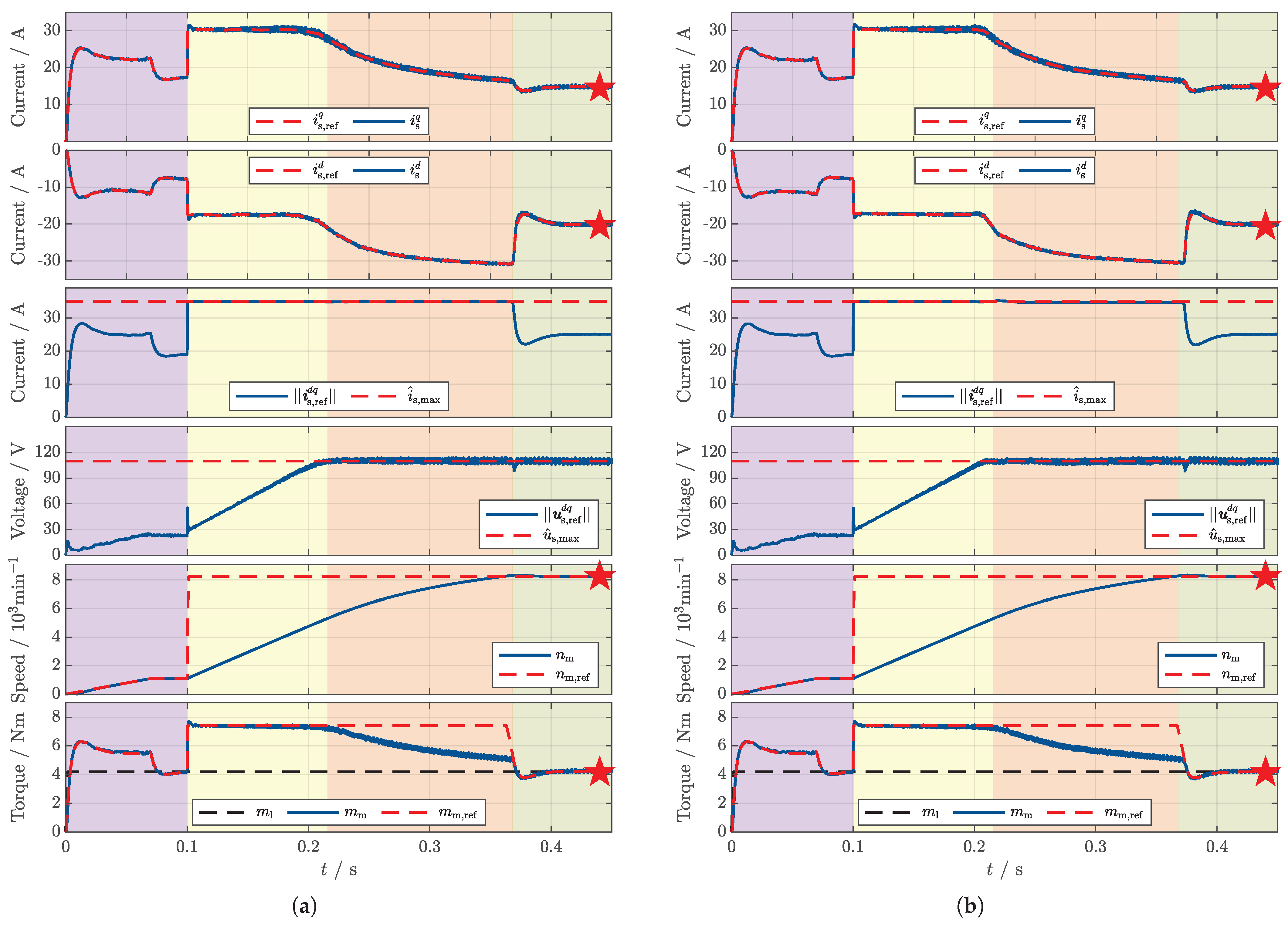
 ], ANN-based OFTC [ ] and OFTC solved directly by fmincon (NLP) [
  ].
], ANN-based OFTC [ ] and OFTC solved directly by fmincon (NLP) [ ].
].
], ANN-based OFTC [ ] and OFTC solved directly by fmincon (NLP) [ ].
| Function Name | Activation Function | Derivative |
|---|---|---|
| Sigmoid | ||
| Tangens hyperbolicus | ||
| Signum (sign) | (not at ) | |
| Identity | ||
| Rectified Linear Unit | ||
| Saturation |
| Description | Architecture (A) | Architecture (A) |
|---|---|---|
| ANN type | Feedforward Neural Network | |
| Model prediction | Regression | |
| Training algorithm | Levenberg-Marquardt | |
| Error function | Mean Squared Error (MSE) | |
| Overall layers | 3 | 4 |
| Hidden layers | 1 | 2 |
| Input vector | ||
| Input neurons | ||
| Input layer activation function | [see Table 1] (without weighting and bias) | |
| Hidden layer activation function | [see Table 1] | |
| Hidden layer neurons | ||
| Output layer activation function | [see Table 1] | |
| Output layer neurons | ||
| Output vector | ||
| Inputs for data set creation: | ||||||||||||
|---|---|---|---|---|---|---|---|---|---|---|---|---|
| Output: Small training set with 10k samples | ||||||||||||
| 14 | 42 | 5 | 110 | 185 | 5 | 0 | 1.6 | 20 | 0 | 2 | 20 | 10k |
| Output: Medium training set with 50k samples | ||||||||||||
| 14 | 42 | 4 | 110 | 185 | 5 | 0 | 1.6 | 50 | 0 | 2 | 50 | 10k |
| Output: Large training set with 200k samples | ||||||||||||
| 14 | 42 | 8 | 110 | 185 | 10 | 0 | 1.6 | 50 | 0 | 2 | 50 | 10k |
| Output: Small validation set with 10k samples | ||||||||||||
| 14 | 42 | 5 | 110 | 185 | 5 | 0 | 1.6 | 20 | 0 | 2 | 20 | 10k |
| Output: Large validation set with 200k samples | ||||||||||||
| 14 | 42 | 8 | 110 | 185 | 10 | 0 | 1.6 | 50 | 0 | 2 | 50 | 10k |
| Scenario | (A) + | (A) + | (A) + |
|---|---|---|---|
| Training duration without normalization (in s) | 136 | 298 | 1450 |
| Training duration with normalization (in s) | 81 | 288 | 937 |
| Relative time reduction (in %) | −40.4% | −3.4% | −35.4% |
| Average time reduction (in %) | −26.4% | ||
| Termination Parameter | Value | Description |
|---|---|---|
| Maximum number of epochs | 400 | Training is terminated if the specified number of epochs is reached (to avoid overfitting and to guarantee termination). |
| Maximum validation failure runs | 10 | Training stops if performance (accuracy) worsens for a certain number of epochs in a row (to avoid overfitting). |
| Maximum training time | ∞ | Training is terminated when the time limit is exceeded (as no computational limit was imposed/required during training and validation). |
| Parameter | Value |
|---|---|
| Operating System | macOS Monterey Version 12.0.1 |
| Processor | 6-Core Intel Core i7 |
| Memory | 162667 DDR4 |
| Graphics | AMD Radeon Pro 5300M 4 |
| IAE of | Time Interval | X = OFTC | X = OFTC | X = OFTC | X = OFTC | |
|---|---|---|---|---|---|---|
| d-current | whole | |||||
| q-current | whole | |||||
| torque | MTPL, MC, FW | |||||
| voltage limit | MC, FW | |||||
| current limit | MC, MC | |||||
| speed | whole | |||||
| mean execution time | one OFTC call |
Publisher’s Note: MDPI stays neutral with regard to jurisdictional claims in published maps and institutional affiliations. |
© 2022 by the authors. Licensee MDPI, Basel, Switzerland. This article is an open access article distributed under the terms and conditions of the Creative Commons Attribution (CC BY) license (https://creativecommons.org/licenses/by/4.0/).
Share and Cite
Buettner, M.A.; Monzen, N.; Hackl, C.M. Artificial Neural Network Based Optimal Feedforward Torque Control of Interior Permanent Magnet Synchronous Machines: A Feasibility Study and Comparison with the State-of-the-Art. Energies 2022, 15, 1838. https://doi.org/10.3390/en15051838
Buettner MA, Monzen N, Hackl CM. Artificial Neural Network Based Optimal Feedforward Torque Control of Interior Permanent Magnet Synchronous Machines: A Feasibility Study and Comparison with the State-of-the-Art. Energies. 2022; 15(5):1838. https://doi.org/10.3390/en15051838
Chicago/Turabian StyleBuettner, Max A., Niklas Monzen, and Christoph M. Hackl. 2022. "Artificial Neural Network Based Optimal Feedforward Torque Control of Interior Permanent Magnet Synchronous Machines: A Feasibility Study and Comparison with the State-of-the-Art" Energies 15, no. 5: 1838. https://doi.org/10.3390/en15051838
APA StyleBuettner, M. A., Monzen, N., & Hackl, C. M. (2022). Artificial Neural Network Based Optimal Feedforward Torque Control of Interior Permanent Magnet Synchronous Machines: A Feasibility Study and Comparison with the State-of-the-Art. Energies, 15(5), 1838. https://doi.org/10.3390/en15051838