Abstract
Energy efficiency is one of the most important current challenges, and its impact at a global level is considerable. To solve current challenges, it is critical that consumers are able to control their energy consumption. In this paper, we propose using a time series of window-based entropy to detect anomalies in the electricity consumption of a household when the pattern of consumption behavior exhibits a change. We compare the accuracy of this approach with two machine learning approaches, random forest and neural networks, and with a statistical approach, the ARIMA model. We study whether these approaches detect the same anomalous periods. These different techniques have been evaluated using a real dataset obtained from different households with different consumption profiles from the Madrid Region. The entropy-based algorithm detects more days classified as anomalous according to context information compared to the other algorithms. This approach has the advantages that it does not require a training period and that it adapts dynamically to changes, except in vacation periods when consumption drops drastically and requires some time for adapting to the new situation.
1. Introduction
In recent years, the interest of people and governments in the energy sector has increased. Society is becoming aware of the importance of environmental sustainability and energy efficiency [1]. The integration of new technologies with power grids has driven a transformation of the energy sector towards a decentralized smart grid. The transition towards the use of smart grids has made it easier to obtain consumption data at different scales. The analysis of this data can have different purposes such as predicting consumption, obtaining consumption patterns, or detecting anomalies, and from this analysis, recommendation systems can be implemented [2].
A household’s electricity consumption is influenced by external variables, such as season, weather, etc., and by internal variables, such as the routines and habits of the dwellers. Additionally, it can be affected by unexpected situations for the dwellers of the household. For example, the restrictions applied during the COVID-19 pandemic caused unexpected socio-economic situations that influenced electricity consumption. The lockdown and restrictions, and the corresponding increase in teleworking and homeschooling, triggered a change in the power consumption profile [3,4].
Previous research [5,6,7] focused on electricity consumption at the national level and studied the impact of the pandemic on electricity demand through forecasting tasks. Hora et al. [8] evaluated different algorithms used in forecasting tasks of atypical consumption behavior. The authors applied these algorithms to household electricity consumption data influenced by the COVID-19 pandemic restrictions. Samara et al. [9] analyzed the impact of the implementation of quarantine measures during the pandemic on electricity consumption in the city of Sharjah. The results show that consumption increased in the residential sector and decreased in sectors such as industry and commerce.
In this work, we collect and analyze electricity consumption data from different households in order to detect anomalies when the behavior pattern changes. By anomaly, we mean a behavior pattern different from the usual, i.e., that does not conform to what is expected or predictable. Our approach is based on the use of entropy. It is an iterative approach, so it allows us to detect changes in the consumption behavior of a household without the need for training. We study whether entropy is able to detect changes in behavior patterns due to unexpected situations.
Entropy is used to detect anomalies in different areas. In previous work, we applied entropy to geolocated traces [10,11]. The performance of the entropy was satisfactory, and it was able to detect anomalies. Entropy is a measure of the uncertainty of a sequence of symbols, and so the information of each symbol is inversely proportional to its probability. One symbol is “predictable” if its probability is high. Applied to electricity consumption, this means that if consumption varies unexpectedly, the symbols should not be predictable and, therefore, the entropy value would change.
To evaluate the results obtained in this study we define two main research questions that we answer in Section 6. The questions are as follows:
- RQ-1: Does entropy detect anomalies in household electricity consumption?
- RQ-2: Do the other approaches detect the same anomalies as entropy?
The remaining of the paper is structured as follows: Section 2 provides an overview of the state of the art related to power consumption traces, power consumption forecasting, and the use of entropy for detecting anomalies. Section 3 describes the methodology followed in this study. Then, Section 4 includes a description of the dataset we collected and the selection of the parameters and different approaches. The results obtained are presented in Section 5. Finally, the conclusions of this paper and future work are presented in Section 6.
2. State of the Art
In this section, we first mention the different methods to obtain electricity consumption traces. Then, we review different works on household electricity consumption forecasting. Later, we review other works that apply entropy in power consumption traces for different purposes. Finally, we review some areas of application of anomaly detection in electricity consumption.
2.1. Electricity Consumption Traces
Thanks to the rise of smart grids and their integration with new technologies, electricity consumption datasets are becoming available. There are three ways to obtain these datasets: traces provided by operators, traces provided by smart meters, and synthetic traces. These datasets may or may not be publicly available and may be aggregated at different levels (device, household, building, group of buildings, city, region, or country).
Table 1 collects different characteristics and the level of detail, aggregated at a household level (Agg.) or at an appliance level (App.), of various publicly available datasets. The duration of the traces is diverse, ranging from days (e.g., REDD) [12] to several years (e.g., Tracebase) [13]. REDD [12] and UK-DALE [14] monitor the aggregate consumption of a few households with a rather high sampling frequency.

Table 1.
Accessible electricity consumption datasets.
In contrast to real traces, synthetic traces allow for modeling the consumption behavior pattern and studying the effect of different characteristics on consumption, such as the use of appliances or the influence of the vacation periods on consumption. Synthetic traces are often based on real traces; e.g., the power consumption model of the appliances presented by Barker et al. [20] was based on data from the Smart* project [19].
2.2. Electricity Consumption Forecasting
Research works that focus on electricity forecasting are becoming more and more frequent. At the same time, the use of machine learning models has also become important in the electricity sector. It should be noted that the diversity of these investigations is wide in the techniques applied, sampling frequency, and time span of the datasets. Besides, the study is conditioned to the extension of the monitored area since the household electricity consumption is influenced by external such as the habits of the dwellers [22].
Jogunola et al. [23] presented a hybrid architecture based on deep learning techniques to predict the electricity consumption of commercial buildings and residential buildings. Chou et al. [24] combined a decomposition method with a prediction algorithm; this approach is applied to buildings with different functionalities located in different time zones. Arvanitidis et al. [25] applied an artificial neural network (ANN) to the Greek power system, taking into account temporal data, temperature, and historical data for forecasting. There are also works on industry consumption forecasting. Leite Coelho da Silva et al. [26] applied statistical approaches and ANN to industrial electricity consumption in the Brazilian system.
Table 2 shows the input characteristics and models applied in some works on household electricity consumption forecasting.
Table 2.
Techniques applied in the forecasting of household electricity consumption.
The regression tree (RT), recurrent neural network (RNN), and support vector regression (SVR) techniques used in [27] obtain similar root mean squared error (RMSE) results, but statistical analysis shows that RT is significantly better. This paper studies the impact of calendar effects on the prediction of consumption and concludes that calendar effects are more important in the absence of historical load information.
Schirmer et al. [30] showed that the approaches that incorporate temporal data (RNN, gated recurrent unit (GRU), and long short-term memory (LSTM)) are more accurate than those that do not (linear regression (LR), DT, deep neural network (DNN)). Compared to the reference model based on linear regression, the LSTM model reduces the mean absolute error (MAE) by up to 26.7%.
Some research focuses on predictions considering meteorological factors. In [29], the authors used outdoor temperature, while [22] took into account different weather characteristics. Wang et al. [22] analyzed different users, and the results showed that weather features increase prediction accuracy. Although this improvement depends on behavior, if users are not susceptible to weather changes, the prediction will not be better.
Other papers propose novel approaches combining different techniques. The approaches presented in [28,31] combine convolutional neural network (CNN) and LSTM, which outperform existing approaches. However, there are recent works that show that the LSTM model can obtain good accuracy in this area [32,33,34].
2.3. Entropy
There are previous works that use entropy in power consumption traces for different purposes. The objective of [35] is to predict electricity consumption, and entropy is used to select the most important input features by a feature selection process (FSP). In [36], outliers in electricity data are detected using an entropy-based approach, used to aggregate data and remove repeated patterns. Kwac et al. [37] propose the use of entropy to capture the variability of customer consumption and to study the daily consumption shape of households. Their conclusion is that entropy could provide a measure of consumption to design a recommendation system.
2.4. Anomalies in Electricity Consumption
The information obtained from anomaly detection in electricity consumption can be used in different areas of application. It could be used to improve the privacy and security of residents. In addition, if there has been no change in the pattern of user behavior, this information can be used for the identification of an appliance failure, a sudden change in the charging system, or fraud in the resident’s electrical system [38].
Electricity consumption data can lead to privacy leaks. Analysis of the data can reveal sensitive information about the behavioral pattern of users, whether an appliance is on or not, whether the dwellers of the household are away, etc. [39]. Im et al. [40] proposed a new method of electricity billing that preserves privacy while preserving data quality. Guan et al. [41] proposed an efficient and privacy-preserving data aggregation scheme.
3. Methodology
In general, energy consumption traces are not well labeled and only provide information on the power consumed. This information is not sufficient to perform an analysis of the consumption behavior pattern. It is important to know what information we have about the household and the dwellers. For this work, we collected electricity consumption traces provided by suppliers to their customers and also information about the households and their dwellers in some households in the Madrid Region (Spain). The dataset used is explained in detail in Section 4.
We applied different approaches to compare the results with the entropy-based approach. We wanted to know which mechanism was most suitable and if entropy performs correctly to detect anomalies. These anomalies will indicate an unusual behavior or a change in the behavior pattern that could be caused, for instance, by a vacation period or a change of job. The dataset from some households covers the pandemic period, including lockdown and restrictions, a situation that interferes with household electricity consumption since most people had their behavior pattern modified. We had the opportunity to study whether the different algorithms detect unexpected situations, as is the case of COVID-19.
3.1. Traditional Algorithms
One method to detect anomalies is the application of algorithms used for forecasting, where machine learning models or statistical models are included. We refer to these models as traditional algorithms. The objective is to predict values after a training period. The expected result is that the real values and the predicted values match. However, if the predicted value deviates from the real value, it can be thought that something unusual has happened in that interval.
The first model we used was random forest (RF) [42]. To control the complexity of the model, parameters that influence the tree construction can be adjusted [43]. Some adjustments limit the depth of the tree or require a minimum number of points at a node to continue splitting. The randomness of the tree is determined by the selection of the features used at each node. Another important parameter is the number of trees used. The more trees, the better, but that influences the performance of the model.
The second model we applied is long short-term memory (LSTM) [44], a type of recurrent neural network (RNN). Building a neural network model is not trivial; one must define the network architecture, the number of layers, and the number of units in each layer, in addition to the activation functions.
The last approach we used was a statistical model based on time series, the auto-regressive integrated moving average (ARIMA) model [45]. We defined the ARIMA (p, d, q) model where p, d, and q are the degrees of the different components of the model: the auto-regressive component, the integrated component, and the moving average component, respectively.
To compare the performance of the different models, we used three common forecasting metrics [46]. The first metric was RMSE. We normalized this error by dividing its value by the mean of the test set, the normalized root mean squared error (NRMSE). Finally, we used a measure of percentage error, the mean absolute percentage error (MAPE).
As described in Section 5, we analyzed the predicted and real values to differentiate an anomalous day from a normal day.
3.2. Entropy
Electricity consumption has a certain degree of randomness because a person’s behavior is not periodic and is influenced by many factors such as occupation or habits. Predictability [47] indicates how foreseeable a user’s behavior is; if the user has a repetitive behavior, it is predictable, while if they have a more random behavior, it is not.
The predictability of a user can be measured by an information theory concept— entropy [48]. A user can be commonly predictable, but then suddenly change its behavior; this behavior results in a change in predictability and, consequently, a change in the value of entropy. Entropy measures the uncertainty of a sequence of symbols, and its definition is as follows:
where X is a discrete random variable whose values belong to an alphabet and is its probability function, the probability mass function (PMF).
Usually, the probability of the symbol, , is calculated as the ratio of the number of occurrences of the symbol to the total length of the sequence. Since we are interested in studying the entropy evolution, we calculate the entropy for each interval (2). We consider from the beginning of the sequence of each interval, i, where the interval is the timestamp.
4. Dataset and Parameter Selection
Before studying the results obtained, we describe the data used in this study and the parameters we adjusted in the different approaches.
4.1. Data Collection
This case study focuses on electricity consumption from 8 households in the Madrid Region (Spain) and on the information obtained about these households and their dwellers (age range, occupation). The electricity consumption data provided by the consumers come from the supplier that provides this information to the consumers. The information related to the home is the zip code, the surface area in square meters, and the presence/absence of different appliances, which are the ones that usually consume more energy or are used more frequently.
The suppliers provide this information to the consumers on their websites. The historical data that the consumer can usually access follow the same scheme: the electricity consumption with its timestamp, the mode of generation of the reading (whether it is real or estimated), and the CUPS of the consumer (i.e., the Universal Supply Point Code in Spain).
We collected the data through a system developed by us. The system allows us to collect data from different consumers. The system considers the existing invoice system in Spain, which allows data collection from all of Spain. The objective is to obtain real electricity consumption traces to process and analyze this data. The processing is in accordance with the General Data Protection Regulation and complies with current data protection regulations.
4.2. Data Description
Table 3 shows the lengths in days of the data for all the households. In all of them, the sampling frequency is one sample per hour.
Table 3.
Length of available data.
When analyzing consumption, it is necessary to take into account the energy consumed in a year, the maximum per hour, and the average per hour in order to compare the households and obtain conclusions. These values, in kWh, can be seen in Table 4.
Table 4.
Description of household loads.
This dataset covers a period including the COVID-19 pandemic. For this reason, we divide the consumption into two periods, the pre-pandemic period up to 14 March 2020 and the pandemic period. In most households, the average consumption was higher in the pandemic period. Figure 1 shows the statistical interpretation of electricity consumption for all households. This interpretation is shown in blue for the pre-pandemic period (up to 14 March 2020) and in pink for the period corresponding to the COVID-19 pandemic.
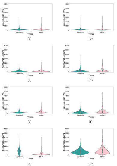
Figure 1.
Statistical interpretation of consumption data (a) H1, (b) H2, (c) H3, (d) H4, (e) H5, (f) H6, (g) H7, and (h) H8.
These figures show the difference in consumption from one period to another. The load distribution in the first five households (H1, H2, H3, H4, and H5) was quite similar, and houses H7 and H8 were significantly different. Although it can be seen that consumption tended to be higher in the COVID-19 period, household H7 followed a different trend, with lower consumption.
In the following study, we focused on households H1 and H2 since we had a longer trace duration, as we can see in Table 3, and the pattern of behavior was different, as shown below in a more detailed study. In addition, more background information about these households allowed us to perform a more in-depth analysis. For these reasons, from this point on, we will focus on the analysis of these two households.
Figure 2 show the total consumption of H1 and H2 during the whole period. The vertical black line on March 14th marks the day when the state of alarm (strict lockdown) was declared in Spain. This line divides the consumption into pre-pandemic and pandemic periods.
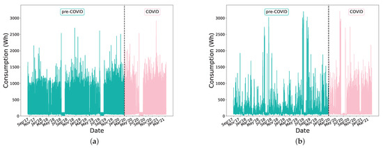
Figure 2.
Consumption of households (a) H1 and (b) H2.
Figure 3 shows the power consumption of H1 and H2, the total consumption of the month, the total consumption of each day of the week, and the hourly consumption of a day. In these figures, the month, day of the week, and time of day with the highest consumption are shown in blue coloring.
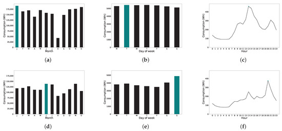
Figure 3.
Average load curves. (a) H1 (monthly). (b) H1 (daily). (c) H1 (hourly). (d) H2 (monthly). (e) H2 (daily). (f) H2 (hourly).
In both households, the month with less power consumption was August, but the month with more consumption in H1 was January and in H2 was June. This explanation lies in the presence of an air conditioner in H2, while H1 had no air conditioner. In H1, consumption was evenly distributed among all days of the week, and consumption was higher at midday. In H2, consumption on weekends was higher than during the labor days, and in the daily consumption curve, we can observe that the peak occurred in the evening. The dwellers of H2 had a full working day and ate away from home during the week.
4.3. Data Analysis
In relation to the granularity of the dataset, the sampling frequency could be less than one hour because our objective was to detect anomalous days. If the sampling frequency was hourly, we obtained too many details of household consumption. We were not interested in knowing the exact time of a peak of consumption, but we did want to study whether the peak occurred in the morning or afternoon. The objective was to reduce the number of samples without losing the information needed for the study. For this reason, we re-sampled the consumption measurements by decreasing the sampling frequency.
We believe that this re-sampling should be automatic. One formal option is to cluster the times of day using a clustering algorithm. In our case, we used the K-means algorithm [49]. First, we obtained the optimal cluster number, the number of slots in which to divide the hours of the day according to their consumption. Then, the K-means algorithm clusters the hours of the day with similar consumptions. From the clusters obtained, we re-sampled the electricity consumption data. To do this, we summed the data and divided it by the number of hours. We decided to calculate the average since the length of periods may not be the same.
4.4. Parameter Selection
As mentioned above, we used three different techniques. The selection of the parameters adjusted in this study is based on different analyses. For the first two models, we defined the same input features to the algorithm: historical data (consumption of the previous day), calendar with the holidays of the Madrid region, and temporal data (time, day of the week, day of the month, and month).
4.4.1. Random Forest
There are several important parameters to consider in this algorithm. In Section 3 we mentioned the parameters that we adjusted. We performed an analysis of the hyperparameters using a grid search based on the out-of-bag (OOB) score. The best combination is shown in Table 5.
Table 5.
Adjusted parameters and OOB score.
However, in Figure 4, the OOB score versus the number of trees shows that the number of estimators undergoes a trade-off with the performance. Therefore, we set the number of estimators equal to 85, at which the score stabilized.
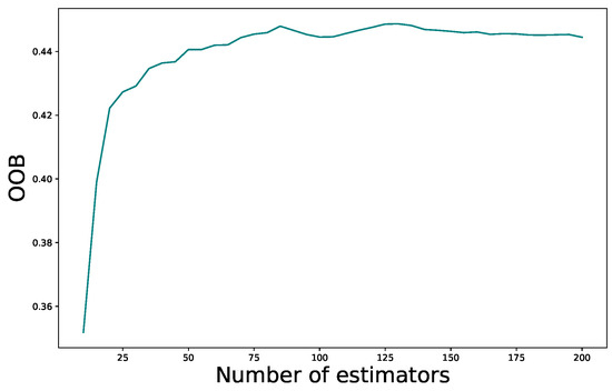
Figure 4.
OOB score vs. number of estimators.
Finally, we set 85 trees, defined the maximum depth of a tree to 10, and set the maximum of features to 3 (1/3 of the total input features). Finally, the minimum number of samples in a node was 3.
4.4.2. Neural Networks
We used an LSTM network with 3 layers. The output layer had a single output since the target variable is consumption and was interconnected with the 9 inputs through a hidden layer.
To select the number of neurons in the hidden layer, we calculated the RMSE from 1 neuron to 25 neurons and selected the model with the best performance. Figure 5 shows the RMSE of each model. We set the number of units to 4 since from this value; the error does not decrease significantly while the model performance degrades.
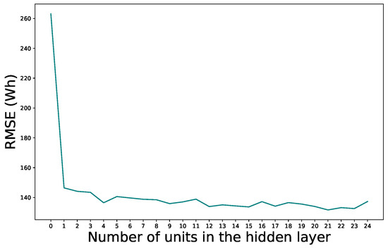
Figure 5.
RMSE vs. number of units.
4.4.3. ARIMA
In the ARIMA model, we defined the three parameters p, d, and q. The first step was to determine whether consumption was stationary or not. If it is, the parameter d would be 0. To this end, we applied the Augmented Dickey Fuller (ADF) test [50], a test of statistical significance. The null hypothesis assumes that the time series is a non-stationary series. We obtained a p-value equal to 6.140 × 10⁻⁵. As this is lower than the significance level, we rejected the null hypothesis and assumed that the series was stationary and d was 0.
To identify the remaining two parameters, p and q, we observed the auto correlation function (ACF) and partial auto correlation function (PACF) figures, respectively, as shown in Figure 6.
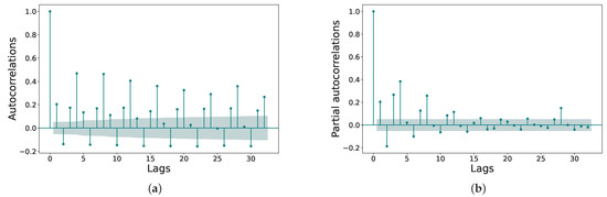
Figure 6.
(a) ACF graph, (b) PACF graph.
According to the obtained correlations, we tentatively identified both parameters at 4, and verified this by comparing the AIC values obtained for the different models. We used an ARIMA model (4, 0, 4).
We applied the same tests to H2 to obtain the parameter values. Table 6 shows the adjusted parameters for both households.
Table 6.
Adjusted parameters of households H1 and H2.
4.5. Entropy
As mentioned in Section 3, the probability of a symbol is calculated as the number of occurrences divided by the length of the sequence. In our sequence of symbols, the length of the alphabet was large because the range of power consumption values was very extensive. Two values with an insignificant difference, such as one watt-hour, are considered to be completely different values. For this reason, before calculating the entropy value, the first step was to discretize the values to increase the accuracy of the entropy. We decided that this clustering should be dynamic, so we used the K-means algorithm with 10 clusters to define the consumption intervals.
Furthermore, we found another issue. The definition of entropy encompasses an infinite series of symbols, so a symbol at the end of this sequence has no impact on the global value of entropy because the past history has a lot of weight in the summation of Equation (2). The blue line in Figure 7 shows this behavior. There came a time when entropy variations were negligible, and the entropy value tended to be almost constant. Therefore, the entropy did not detect any different behaviors. An anomalous behavior would have to be very long to have an influence on the entropy. To solve this issue, we took into account the most recent past in each interval.
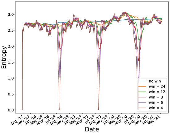
Figure 7.
Entropy of household H1.
We calculated the entropy value within a sliding window, in which we only considered the last symbols of the sequence. We defined different window sizes, short enough to detect changes in user predictability and consumption, but large enough to add some past memory.
Figure 7 shows the entropy evolution of H1 with different window sizes. The window ranged from 4 weeks, which corresponds to the brown line, to 24 weeks (orange line). If the window size was small, the entropy variations were more significant because there were few samples, and any unexpected events would be reflected. From this point on, we considered a 6-week window to perform the calculations, as we believe it is an average timeframe and is long enough to detect changes in consumption.
5. Results and Discussion
In this section, we discuss the results obtained using traditional algorithms and using the entropy-based approach. The first step is to apply the different approaches to a period prior to COVID-19, specifically, the period corresponding to the year 2019–2020. To study periods of the same length in both houses, we considered one year before 14 March 2020.
5.1. Traditional Algorithms
With the RF and LSTM models, the first step was to divide the dataset into a training part and a test part—the training part from September 2017 to March 2019 and the test part until March 2020. The split corresponds to 60% and 40%, respectively. We tested with different training sizes, and 60–40 detected the most anomalous days. Then, we transformed the data to obtain an input matrix to the algorithm with the required features, target variable, and consumption in each interval. The next step was to create the model and fit it with the training data. Once both models were created and adjusted, we performed the consumption forecasting.
The main purpose was to obtain the days in which the prediction did not match the real data. We were interested in knowing the intervals in which the prediction was not correct. If the predicted value differed from the true value, we would think that something unusual was happening. We calculated the difference in absolute value between the predicted values and the true values. Next, we needed to set a threshold on this difference to separate the abnormal days from the normal days. The distribution of discrepancies between the actual and predicted values from the RF algorithm in H1 were concentrated in values below 200 Wh.
The number of days considered anomalous depends on the set limit; the number of days decreases as the limit is increased. In addition, to set this limit, we had to take into account the average consumption of the household, so this limit was different for each one. According to the graphs, we believe that it is a good estimate to establish the limit in the average consumption of this interval.
However, if we only look at this difference, we consider too many days as anomalous that, for us, would not be anomalous. Therefore, this criterion is not enough. Additionally, we studied the slope of consumption in each interval, since we were interested in the trend of consumption. We set the following criterion: the difference between the consumption in each interval with respect to the previous interval must follow the same trend; it must be increasing or decreasing in real values and predicted values. If they do not follow the same trend, it may indicate that something strange has happened.
In summary, we establish that in order to consider a day as anomalous, both conditions must be met: the first one is that the difference between the true value and predicted value must differ more than the average consumption; the second one is that the trend of each reading must be different in the actual values and the predicted values.
With these criteria, in H1, the RF detected 27 anomalous days; the neural network model, 27; and the ARIMA model, 37. From the union of all these anomalous days, there were 15 detected by the three algorithms and another 15 detected by two of them.
In H2, the RF detected 19 anomalous days; LSTM, 32; and ARIMA, 39. If we look at the errors obtained in the predictions, the RF was the model with the lowest error. In this case, 11 anomalies were detected by the three approaches and 12 by two of them.
5.2. Our Approach
To obtain the anomalous days, we studied the evolution of entropy. In Figure 8, we observe the evolution of entropy in both households. In the entropy of H1, we can observe three sudden drops that correspond to the summer periods during the month of August. These variations can be visualized in their consumption (Figure 2a). H1 presents a more repetitive trend in electricity consumption and entropy evolution.
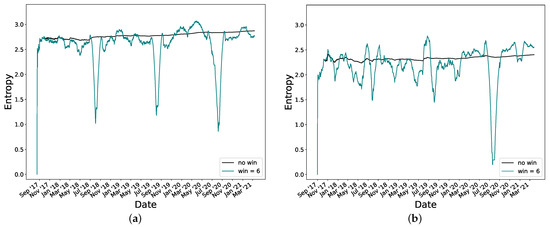
Figure 8.
Entropy of households (a) H1 and (b) H2.
We obtained the difference of entropy in each interval with respect to the previous value, and we ordered the values obtained in descending order—the greater the difference, the greater the change. In Figure 9, we see the days ordered according to the entropy difference from the rarest day to the least rare day, or most “normal” day, in H1.
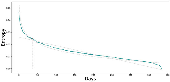
Figure 9.
Days ordered by entropy value.
We needed to set a threshold at which we considered the days as anomalous or normal. To establish the threshold, we fit two trend lines, a linear trend and a logarithmic trend—both lines can be seen in Figure 9 in dashed gray. The intersection point between both lines was the threshold to differentiate the anomalous days. In this case, the threshold was 37.
We obtained the date corresponding to the anomalous days and made a classification from the most anomalous day to the least anomalous (or most normal). We then made a more detailed analysis of the anomalies detected and compared the results with the anomalies obtained by the different approaches.
5.3. Comparison and Discussion
We studied the anomalies detected by each algorithm and compared the results obtained. We differentiated between anomalies detected by entropy alone and anomalies detected by the entropy and one or more of the alternative approaches.
5.3.1. Household H1
Table 7 shows the anomalies of H1 detected by entropy and by one or more of the implemented algorithms. The days are sorted from the most anomalous to the least anomalous, according to the classification of anomalous days obtained by the entropy approach. The last column, “ground truth”, indicates whether the dates detected as anomalous were actually rare or unusual, according to the dwellers.
Table 7.
Anomalous Days of Household H1.
The percentage of days detecting entropy, which is also detected by each of the different approaches, were as follows: 43% (RF), 38% (LSTM), and 49% (ARIMA). The different approaches may not detect the same days, but they do detect adjacent days that correspond to anomalous periods. Only three anomalies detected by the different techniques were not really anomalous periods.
The days detected only by the entropy-based approach corresponded to the vacation period and the following days, specifically the days in August and September. These days correspond to the sudden change in entropy. The entropy approach does not adapt immediately since the holiday period is long and continues to flag days as anomalous until it adjusts again.
Traditional algorithms detect and learn the pattern of consumption behavior. In H1, during the month of August, these algorithms did not mark any days as anomalous because it learned from previous years, and the vacation pattern was quite periodic.
5.3.2. Household H2
As in H1, we compared the anomalies detected by the different approaches. The anomalies detected in H2 are shown in Table 8.
Table 8.
Anomalous days of household H2.
In H2, approximately 55% of the anomalous periods shown in Table 8 were actually anomalous, according to the dwellers. The remaining periods correspond to apparently normal days. Specifically, 25% of the days detected as anomalous by the ARIMA model coincided with weekends, detecting these periods as “abnormal” when they should have been normal. In H1, the same did not happen because the behavior pattern was similar all week, while in H2, a difference was observed during the weekends. The percentages of anomalous days detected by the entropy, which were also detected by each of the other approaches, were as follows: 30% (RF), 46% (LSTM), and 49% (ARIMA).
As we might expect, when we compared the anomalies detected in both households, there was no relationship between them since H1 and H2 had a different pattern of consumption behavior. For example, H1 had a more repetitive and constant behavior than H2. There were three periods detected by both households that corresponded to the end of the academic year (end of June), the beginning of the school year (beginning of September), and the beginning of the Christmas vacations.
5.4. Pandemic Period
We applied the same methodology to the pandemic period from March 2020 to March 2021. We expected the traditional algorithms to detect more anomalous days due to the change in routine of the dwellers and, nevertheless, in H1, the algorithms detected very few days as anomalous compared to the previous results. This means that, at first, we could assume that COVID-19 had a large impact on household electricity consumption, but depended on the dwellers.
In H2, the opposite occurred. The LSTM model, for example, detected 48 anomalies concentrated in the last months of 2020 and the beginning of 2021. If we look at the consumption of H2 in Figure 2b, it is evident that it did not follow the same pattern as in previous years.
In this year, in H1 and H2, the vacation period away from home was longer; therefore, about 50% of the days were detected as anomalous by the entropy approach corresponding to August and September. The same happened in the pre-COVID period in H1.
Another conclusion we obtained was that during the total lockdown, from the beginning (March 15th) to mid-June, the entropy approach did not detect any day as anomalous since all the days were similar—there was no difference in the pattern of behavior in the days of the week. Of the 37 anomalies, only 3 days coincided with the total lockdown in H1 and 2 days in H2.
Finally, if we look at Figure 8, we can observe an increase in entropy in the 2020 period, corresponding to the pandemic, with respect to previous years. This increase is evident and means that something strange happened during these months. This change indicates that consumers changed their power consumption habits considerably.
5.5. Other Households
In this section, we analyze and discuss the results obtained in the remaining households, H3 through H8. In this case, we have not divided the consumption into two different periods because we did not have enough data to make accurate predictions. We performed this analysis separately for households H1 and H2. The monitored period started almost simultaneously in houses H3 to H8, a few months or days before the start of the pandemic; for this reason, we decided to perform the training with 60% of the final data. Therefore, the period concerning the total lockdown was part of the test period.
Table 9 shows the number of anomalous days that the entropy approach detects and the percentage of these days, which is also detected by each other approach (RF, LSTM, and ARIMA).
Table 9.
Anomalous days of households.
Entropy detects a higher number of anomalies in households H4 and H5 because the period monitored in both households was twice as long as in the remaining households. In addition, in these households, the percentage of days detected by the entropy approach and by another approach was higher—in all six cases, almost exceeding 50%.
In the case of households H3, H6, and H8, the percentage did not exceed 15%, which means that the anomalies detected using the entropy were not detected by the other approaches. It should be noted that RF in H6 did not detect any anomaly.
6. Conclusions
In this work, we use different approaches to detect anomalies in the electricity consumption of a household: two machine learning methods, a statistical approach, and an entropy-based approach. In the entropy approach, we consider the last weeks using a sliding window to study the predictability of users. The different approaches have been tested on a real dataset obtained from different households in the Madrid Region, with different load profiles.
Although we analyzed in detail the results obtained in two households, the conclusions extracted in the remaining households were similar. Furthermore, although we used data from the Madrid Region, we consider that the conclusions can be extrapolated to other regions.
To evaluate whether we have fulfilled the objectives, we answer the research questions proposed in Section 1:
- RQ-1: Does entropy detect anomalies in household electricity consumption?
As mentioned in the previous section, entropy is able to help detect anomalous periods in the consumption of a household. We studied the behavior pattern of two households with different power consumption patterns, and in both of them, it detected anomalous periods. In H1, only three anomalies detected by the different techniques were not real anomalies. The days detected just by the entropy-based approach correspond to the vacation period and the next days. In H2, around 55% of the anomalous periods detected by the different techniques are real anomalies. In both households, during the total lockdown, using entropy, we did not detect any day as anomalous since all the days were similar, and there was no difference in the pattern of behavior in the days of the week.
- RQ-2: Do the other approaches detect the same anomalies as entropy?
The other approaches also detected anomalies, sometimes not exactly the same anomalous days as entropy, but adjacent days. This means that something happened in household consumption, such as a weekend trip. A supplier with many customers could detect anomalous periods in household electricity consumption, regardless of the exact day. The percentages of days detected using entropy, which were also detected by each of the other approaches, were as follows: in H1, the percentage for RF was 43%, 38% for LSTM, and 49% for ARIMA. In H2, the percentages were similar: 30% (RF), 46% (LSTM), and 49% (ARIMA).
The advantage of the entropy-based approach was the absence of a training phase, which implies that the algorithm is able to detect anomalous behavior from the beginning. However, it starts to obtain good results from the last 6 weeks onward, depending on the size of the window. Thanks to the window, the entropy adapts dynamically to changes in the consumption pattern, although it has certain limitations.
One limitation of the entropy approach is the adaptation to changes when consumption changes significantly during a long period of time. This is the case of long-term vacations when consumption is practically 0; in such situations, entropy does not adapt immediately. On the other hand, if this vacation period is repeated periodically, traditional algorithms do not classify these periods as anomalous. Machine learning techniques detect and learn behavioral patterns dependent on temporal information, such as time or day of the week, but the entropy does not take into account the temporal frequency of consumption.
The entropy mechanism allows the detection of anomalies in electricity consumption. The user can then study the cause of these anomalies. If there has been no change in their pattern of behavior, the anomaly may be due to a failure of an appliance or a sudden change in tariffs. The user can take advantage of this information to change her habits and thus reduce her power consumption and, therefore, the associated costs.
As future work, it would be interesting to apply this methodology to more households and to expand the number of approaches implemented. Another alternative would be to create a synthetic dataset from this dataset. Future work should compare the results with a hybrid method, which can be selected from [51,52] and from the literature review performed in [28].
Author Contributions
Conceptualization, C.C. and C.G.-R.; methodology, C.C. and C.G.-R.; software, M.M.-G.; validation, M.M.-G., C.C. and C.G.-R.; formal analysis, C.C. and C.G.-R.; investigation, M.M.-G.; data curation, M.M.-G.; writing—original draft preparation, M.M.-G.; writing—review and editing, M.M.-G., C.C. and C.G.-R.; visualization, M.M.-G.; funding acquisition, C.C. and C.G.-R. All authors have read and agreed to the published version of the manuscript.
Funding
This research was funded by Spanish Government under the research project "Enhancing Communication Protocols with Machine Learning while Protecting Sensitive Data (COMPROMISE)" (PID2020-113795RB-C32 MCIN/AEI/10.13039/501100011033).
Institutional Review Board Statement
Not applicable.
Informed Consent Statement
Not applicable.
Data Availability Statement
Not applicable.
Acknowledgments
This work was supported by the Spanish Government under the research project “Enhancing Communication Protocols with Machine Learning while Protecting Sensitive Data (COMPROMISE)” (PID2020-113795RB-C32 MCIN/AEI/10.13039/501100011033) and the project MAGOS (TEC2017-84197-C4-1-R), and by the Comunidad de Madrid (Spain) under the projects: CYNAMON (P2018/TCS-4566), co-financed by the European Structural Funds (ESF and FEDER), and the Multiannual Agreement with UC3M in the line of Excellence of University Professors (EPUC3M21), in the context of the V PRICIT (Regional Programme of Research and Technological Innovation).
Conflicts of Interest
The authors declare no conflict of interest. The funders had no role in the design of the study; in the collection, analyses, or interpretation of data; in the writing of the manuscript, or in the decision to publish the results.
Abbreviations
The following abbreviations are used in this manuscript:
| ARIMA | Auto-Regressive Integrated Moving Average |
| CNN | Convolutional Neural Network |
| DNN | Deep Neural Network |
| DT | Decision Tree |
| GRU | Gated Recurrent Unit |
| LR | Linear Regression |
| LSTM | Long Short-Term Memory |
| MAPE | Mean Absolute Percentage Error |
| MLP | Multi-Layer Perceptron |
| MLR | Multiple Linear Regression |
| NRMSE | Normalized Root Mean Squared Error |
| RF | Random Forest |
| RMSE | Root Mean Squared Error |
| RNN | Recurrent Neural Network |
| RT | Regression Tree |
| SVR | Support Vector Regression |
| Wh | Watt Hour |
References
- Rau, H.; Moran, P.; Manton, R.; Goggins, J. Changing energy cultures? Household energy use before and after a building energy efficiency retrofit. Sustain. Cities Soc. 2020, 54, 101983. [Google Scholar] [CrossRef]
- Himeur, Y.; Ghanem, K.; Alsalemi, A.; Bensaali, F.; Amira, A. Artificial intelligence based anomaly detection of energy consumption in buildings: A review, current trends and new perspectives. Appl. Energy 2021, 287, 116601. [Google Scholar] [CrossRef]
- Navon, A.; Machlev, R.; Carmon, D.; Onile, A.E.; Belikov, J.; Levron, Y. Effects of the COVID-19 Pandemic on Energy Systems and Electric Power Grids—A Review of the Challenges Ahead. Energies 2021, 14, 1056. [Google Scholar] [CrossRef]
- Ghiani, E.; Galici, M.; Mureddu, M.; Pilo, F. Impact on Electricity Consumption and Market Pricing of Energy and Ancillary Services during Pandemic of COVID-19 in Italy. Energies 2020, 13, 3357. [Google Scholar] [CrossRef]
- Tudose, A.M.; Picioroaga, I.I.; Sidea, D.O.; Bulac, C.; Boicea, V.A. Short-Term Load Forecasting Using Convolutional Neural Networks in COVID-19 Context: The Romanian Case Study. Energies 2021, 14, 4046. [Google Scholar] [CrossRef]
- Alasali, F.; Nusair, K.; Alhmoud, L.; Zarour, E. Impact of the COVID-19 Pandemic on Electricity Demand and Load Forecasting. Sustainability 2021, 13, 1435. [Google Scholar] [CrossRef]
- Obst, D.; de Vilmarest, J.; Goude, Y. Adaptive Methods for Short-Term Electricity Load Forecasting During COVID-19 Lockdown in France. IEEE Trans. Power Syst. 2021, 36, 4754–4763. [Google Scholar] [CrossRef]
- Hora, C.; Dan, F.C.; Bendea, G.; Secui, C. Residential Short-Term Load Forecasting during Atypical Consumption Behavior. Energies 2022, 15, 291. [Google Scholar] [CrossRef]
- Samara, F.; Abu-Nabah, B.A.; El-Damaty, W.; Bardan, M.A. Assessment of the Impact of the Human Coronavirus (COVID-19) Lockdown on the Energy Sector: A Case Study of Sharjah, UAE. Energies 2022, 15, 1496. [Google Scholar] [CrossRef]
- Rodriguez Carrión, A.; Garcia-Rubio, C.; Campo, C. Detecting and Reducing Biases in Cellular-Based Mobility Data Sets. Entropy 2018, 20, 736. [Google Scholar] [CrossRef] [Green Version]
- Garcia-Rubio, C.; Díaz Redondo, R.; Campo, C.; Fernández Vilas, A. Using entropy of social media location data for the detection of crowd dynamics anomalies. Electronics 2018, 7, 380. [Google Scholar] [CrossRef] [Green Version]
- Kolter, J.Z.; Johnson, M.J. REDD: A public data set for energy disaggregation research. In Proceedings of the Workshop on Data Mining Applications in Sustainability (SIGKDD), San Diego, CA, USA, 21 August 2011; Volume 25, pp. 59–62. [Google Scholar]
- Reinhardt, A.; Baumann, P.; Burgstahler, D.; Hollick, M.; Chonov, H.; Werner, M.; Steinmetz, R. On the accuracy of appliance identification based on distributed load metering data. In Proceedings of the 2012 Sustainable Internet and ICT for Sustainability (SustainIT), Pisa, Italy, 4–5 October 2012; pp. 1–9. [Google Scholar]
- Kelly, J.; Knottenbelt, W. The UK-DALE dataset, domestic appliance-level electricity demand and whole-house demand from five UK homes. Sci. Data 2015, 2, 150007. [Google Scholar] [CrossRef] [PubMed] [Green Version]
- Makonin, S.; Ellert, B.; Bajić, I.V.; Popowich, F. Electricity, water, and natural gas consumption of a residential house in Canada from 2012 to 2014. Sci. Data 2016, 3, 160037. [Google Scholar] [CrossRef] [PubMed] [Green Version]
- Beckel, C.; Kleiminger, W.; Cicchetti, R.; Staake, T.; Santini, S. The ECO data set and the performance of non-intrusive load monitoring algorithms. In Proceedings of the 1st ACM Conference on Embedded Systems for Energy-Efficient Buildings, ACM, Memphis, TN, USA, 3–6 November 2014; pp. 80–89. [Google Scholar]
- Monacchi, A.; Egarter, D.; Elmenreich, W.; D’Alessandro, S.; Tonello, A.M. GREEND: An energy consumption dataset of households in Italy and Austria. In Proceedings of the 2014 IEEE International Conference on Smart Grid Communications (SmartGridComm), IEEE, Venice, Italy, 3–6 November 2014; pp. 511–516. [Google Scholar]
- Murray, D.; Stankovic, L.; Stankovic, V. An electrical load measurements dataset of United Kingdom households from a two-year longitudinal study. Sci. Data 2017, 4, 160122. [Google Scholar] [CrossRef] [PubMed] [Green Version]
- Barker, S.; Mishra, A.; Irwin, D.; Cecchet, E.; Shenoy, P.; Albrecht, J. Smart*: An open data set and tools for enabling research in sustainable homes. SustKDD August 2012, 111, 108. [Google Scholar]
- Barker, S.; Kalra, S.; Irwin, D.; Shenoy, P. Empirical characterization and modeling of electrical loads in smart homes. In Proceedings of the 2013 International Green Computing Conference Proceedings, Arlington, VA, USA, 27–29 June 2013; pp. 1–10. [Google Scholar]
- Klemenjak, C.; Kovatsch, C.; Herold, M.; Elmenreich, W. A synthetic energy dataset for non-intrusive load monitoring in households. Sci. Data 2020, 7, 1–17. [Google Scholar] [CrossRef] [PubMed] [Green Version]
- Wang, Y.; Zhang, N.; Chen, X. A Short-Term Residential Load Forecasting Model Based on LSTM Recurrent Neural Network Considering Weather Features. Energies 2021, 14, 2737. [Google Scholar] [CrossRef]
- Jogunola, O.; Adebisi, B.; Hoang, K.V.; Tsado, Y.; Popoola, S.I.; Hammoudeh, M.; Nawaz, R. CBLSTM-AE: A Hybrid Deep Learning Framework for Predicting Energy Consumption. Energies 2022, 15, 810. [Google Scholar] [CrossRef]
- Chou, S.Y.; Dewabharata, A.; Zulvia, F.E.; Fadil, M. Forecasting Building Energy Consumption Using Ensemble Empirical Mode Decomposition, Wavelet Transformation, and Long Short-Term Memory Algorithms. Energies 2022, 15, 1035. [Google Scholar] [CrossRef]
- Arvanitidis, A.I.; Bargiotas, D.; Daskalopulu, A.; Laitsos, V.M.; Tsoukalas, L.H. Enhanced Short-Term Load Forecasting Using Artificial Neural Networks. Energies 2021, 14, 7788. [Google Scholar] [CrossRef]
- Leite Coelho da Silva, F.; da Costa, K.; Canas Rodrigues, P.; Salas, R.; López-Gonzales, J.L. Statistical and Artificial Neural Networks Models for Electricity Consumption Forecasting in the Brazilian Industrial Sector. Energies 2022, 15, 588. [Google Scholar] [CrossRef]
- Lusis, P.; Khalilpour, K.R.; Andrew, L.; Liebman, A. Short-term residential load forecasting: Impact of calendar effects and forecast granularity. Appl. Energy 2017, 205, 654–669. [Google Scholar] [CrossRef]
- Yan, K.; Wang, X.; Du, Y.; Jin, N.; Huang, H.; Zhou, H. Multi-step short-term power consumption forecasting with a hybrid deep learning strategy. Energies 2018, 11, 3089. [Google Scholar] [CrossRef] [Green Version]
- Gerossier, A.; Girard, R.; Bocquet, A.; Kariniotakis, G. Robust Day-Ahead Forecasting of Household Electricity Demand and Operational Challenges. Energies 2018, 11, 3503. [Google Scholar] [CrossRef] [Green Version]
- Schirmer, P.A.; Mporas, I.; Potamitis, I. Evaluation of regression algorithms in residential energy consumption prediction. In Proceedings of the 2019 3rd European Conference on Electrical Engineering and Computer Science (EECS), Athens, Greece, 28–30 December 2019; pp. 22–25. [Google Scholar]
- Kim, T.Y.; Cho, S.B. Predicting residential energy consumption using CNN-LSTM neural networks. Energy 2019, 182, 72–81. [Google Scholar] [CrossRef]
- Shi, H.; Xu, M.; Li, R. Deep Learning for Household Load Forecasting—A Novel Pooling Deep RNN. IEEE Trans. Smart Grid 2018, 9, 5271–5280. [Google Scholar] [CrossRef]
- Kong, W.; Dong, Z.Y.; Jia, Y.; Hill, D.J.; Xu, Y.; Zhang, Y. Short-Term Residential Load Forecasting Based on LSTM Recurrent Neural Network. IEEE Trans. Smart Grid 2019, 10, 841–851. [Google Scholar] [CrossRef]
- Hou, T.; Fang, R.; Tang, J.; Ge, G.; Yang, D.; Liu, J.; Zhang, W. A Novel Short-Term Residential Electric Load Forecasting Method Based on Adaptive Load Aggregation and Deep Learning Algorithms. Energies 2021, 14, 7820. [Google Scholar] [CrossRef]
- Jurado, S.; Nebot, À.; Mugica, F.; Avellana, N. Hybrid methodologies for electricity load forecasting: Entropy-based feature selection with machine learning and soft computing techniques. Energy 2015, 86, 276–291. [Google Scholar] [CrossRef] [Green Version]
- Hock, D.; Kappes, M.; Ghita, B. Using multiple data sources to detect manipulated electricity meter by an entropy-inspired metric. Sustain. Energy Grids Netw. 2020, 21, 100290. [Google Scholar] [CrossRef]
- Kwac, J.; Flora, J.; Rajagopal, R. Household energy consumption segmentation using hourly data. IEEE Trans. Smart Grid 2014, 5, 420–430. [Google Scholar] [CrossRef]
- Oprea, S.V.; Bâra, A.; Puican, F.C.; Radu, I.C. Anomaly Detection with Machine Learning Algorithms and Big Data in Electricity Consumption. Sustainability 2021, 13, 963. [Google Scholar] [CrossRef]
- Chen, Y.; Martínez, J.F.; Castillejo, P.; López, L. A Privacy-Preserving Noise Addition Data Aggregation Scheme for Smart Grid. Energies 2018, 11, 2972. [Google Scholar] [CrossRef] [Green Version]
- Im, J.H.; Kwon, H.Y.; Jeon, S.Y.; Lee, M.K. Privacy-Preserving Electricity Billing System Using Functional Encryption. Energies 2019, 12, 1237. [Google Scholar] [CrossRef] [Green Version]
- Guan, Z.; Si, G.; Zhang, X.; Wu, L.; Guizani, N.; Du, X.; Ma, Y. Privacy-Preserving and Efficient Aggregation Based on Blockchain for Power Grid Communications in Smart Communities. IEEE Commun. Mag. 2018, 56, 82–88. [Google Scholar] [CrossRef] [Green Version]
- Breiman, L. Random forests. Mach. Learn. 2001, 45, 5–32. [Google Scholar] [CrossRef] [Green Version]
- Müller, A.C.; Guido, S. Introduction to Machine Learning with Python: A Guide for Data Scientists; O’Reilly Media, Inc.: Sebastopol, CA, USA, 2016. [Google Scholar]
- Hochreiter, S.; Schmidhuber, J. Long short-term memory. Neural Comput. 1997, 9, 1735–1780. [Google Scholar] [CrossRef]
- Hamilton, J.D. Time Series Analysis; Princeton University Press: Princeton, NJ, USA, 1994. [Google Scholar]
- Hyndman, R.J.; Koehler, A.B. Another look at measures of forecast accuracy. Int. J. Forecast. 2006, 22, 679–688. [Google Scholar] [CrossRef] [Green Version]
- Song, C.; Qu, Z.; Blumm, N.; Barabási, A.L. Limits of predictability in human mobility. Science 2010, 327, 1018–1021. [Google Scholar] [CrossRef] [PubMed] [Green Version]
- Cover, T.M.; Thomas, J.A. Elements of Information Theory; John Wiley & Sons: Hoboken, NJ, USA, 2012. [Google Scholar]
- MacQueen, J. Some methods for classification and analysis of multivariate observations. In Proceedings of the Fifth Berkeley Symposium on Mathematical Statistics and Probability, Oakland, CA, USA, 1 January 1967; Volume 1, pp. 281–297. [Google Scholar]
- Dickey, D.A.; Fuller, W.A. Distribution of the estimators for autoregressive time series with a unit root. J. Am. Stat. Assoc. 1979, 74, 427–431. [Google Scholar]
- Debnath, K.B.; Mourshed, M. Forecasting methods in energy planning models. Renew. Sustain. Energy Rev. 2018, 88, 297–325. [Google Scholar] [CrossRef] [Green Version]
- Vivas, E.; Allende-Cid, H.; Salas, R. A Systematic Review of Statistical and Machine Learning Methods for Electrical Power Forecasting with Reported MAPE Score. Entropy 2020, 22, 1412. [Google Scholar] [CrossRef] [PubMed]
Publisher’s Note: MDPI stays neutral with regard to jurisdictional claims in published maps and institutional affiliations. |
© 2022 by the authors. Licensee MDPI, Basel, Switzerland. This article is an open access article distributed under the terms and conditions of the Creative Commons Attribution (CC BY) license (https://creativecommons.org/licenses/by/4.0/).