Multi-Step Short-Term Building Energy Consumption Forecasting Based on Singular Spectrum Analysis and Hybrid Neural Network

Abstract

Short-term building energy consumption forecasting is vital for energy conservation and emission reduction. However, it is challenging to achieve accurate short-term forecasting of building energy consumption due to its nonlinear and non-stationary characteristics. This paper proposes a novel hybrid short-term building energy consumption forecasting model, SSA-CNNBiGRU, which is the integration of SSA (singular spectrum analysis), a CNN (convolutional neural network), and a BiGRU (bidirectional gated recurrent unit) neural network. In the proposed SSA-CNNBiGRU model, SSA is used to decompose trend and periodic components from the original building energy consumption data to reconstruct subsequences, the CNN is used to extract deep characteristic information from each subsequence, and the BiGRU network is used to model the dynamic features extracted by the CNN for time series forecasting. The subsequence forecasting results are superimposed to obtain the predicted building energy consumption results. Real-world electricity and natural gas consumption datasets of office buildings in the UK were studied, and the multi-step ahead forecasting was carried out under three different scenarios. The simulation results indicate that the proposed model can improve building energy consumption forecasting accuracy and stability.

1. Introduction

Against the background of increasing global population and rapid economic development, the energy demand for buildings has increased significantly [1]. According to the World Watch Institute, public buildings account for one-third of global energy consumption and nearly 40% of carbon dioxide emissions each year [2]. The high percentage of energy consumption in buildings has caused significant environmental issues, such as climate warming and air pollution, seriously impacting human survival. As the key to energy management, building energy consumption prediction realizes energy conservation and emission reduction through decision making [3]. However, due to the uncertainty caused by time-varied building operation and environmental conditions, it is usually challenging to forecast building energy consumption accurately [4]. Therefore, it is essential to create a robust model that can capture building energy consumption changes and provide accurate building management information [5].

According to the forecast horizon, building energy consumption prediction is generally classified into ultra-short-term, short-term, medium-term, and long-term predictions [6]. In addition, short-term building energy consumption prediction is closely related to the daily operation mode of the energy system, which can provide users with economic energy conservation measures and practical guidance [7]. According to the results of short-term forecasting, the future short-term operation mode of building energy systems can be adjusted to achieve better resource allocation, which is of great significance to achieving the goal of smart grid infrastructure [8,9]. Therefore, short-term prediction of building energy consumption has become the focus of current research.

In the past decade, relying on the booming development of smart grid technology worldwide, the installation and application of a large number of sensors represented by smart meters has greatly improved the observability of power grids, and the power industry has accumulated massive historical data on building energy consumption [10]. At the same time, the performance of computers has improved explosively with the updating of microprocessors every few years, which has caused the disadvantages of traditional prediction methods, which cannot make full use of big data and computing power, to gradually become exposed. On the contrary, neural network algorithms have been widely applied in prediction due to the advantages of nonlinear mapping and self-adaptation [11]. As one of the most representative deep neural networks, CNNs perform feature extraction of data through convolution and pooling operations to reduce errors caused by artificial feature extraction, making them widely used in image recognition and speech translation [12]. LSTM (long short-term memory) has more robust adaptability to sequential data than traditional recurrent neural networks as an improved recurrent neural network [13]. However, an LSTM network has more parameters and a slower convergence speed. GRU is an optimized network based on LSTM that simplifies the internal unit structure of LSTM to shorten the convergence time [14]. However, a GRU network only considers the influence of historical factors on the prediction results. In fact, energy consumption is not only determined by historical consumption factors, but it is also associated with consumption factors in the future. Moreover, a GRU network still has the disadvantage of not fully exploring the effective potential relationships among energy consumption characteristics. Therefore, we considered the combination of CNN and BiGRU networks to improve the extraction ability of energy consumption characteristics.

In addition, building energy consumption has strong randomness and volatility characteristics, and it is often affected by many interference factors, which make filtering processing technology an essential stage of data preprocessing. As a powerful data denoising technology, SSA has been applied to load prediction [15,16], hydrological prediction [17], wind speed prediction [18,19], and other fields. Experimental results of the relevant literature showed that SSA is superior to empirical mode decomposition and wavelet decomposition in noise reduction [20].

Based on the above considerations, we proposed an SSA-CNNBiGRU model for short-term prediction of building energy consumption. Firstly, the original energy consumption data was decomposed and denoised by SSA, and $N$ characteristic subsequences with the largest contributions to the original sequence were extracted. Secondly, a CNNBiGRU model was used for feature extraction and time series prediction for each subsequence. Finally, the prediction results of each subsequence were superimposed as energy consumption prediction results. After simulations with real-world building energy consumption datasets, we proved that the proposed model has excellent prediction accuracy and stability and can be applied to the short-term prediction of building energy consumption. The main contributions of the paper are as follows:

• We proposed a new hybrid neural network model for real-world building energy consumption forecasting based on SSA. Compared with traditional forecasting models, the proposed model achieved the highest prediction accuracy and had stronger peak and valley capture ability, which effectively alleviated the lag of extreme point data forecasting;
• The simulation results demonstrated that the proposed model still had excellent forecasting precision and stability in the multi-step ahead forecasting scenario, meeting the basic building energy consumption forecasting requirements;
• We compared and analyzed the forecasting effects of neural network models optimized by five decomposition algorithms in the multi-step ahead forecasting scenario. The simulation results showed that the SSA method was a suitable feature extractor that reduced the computational burden and improved the forecast accuracy of the model.

The remainder of the paper is organized as follows: Section 2 discusses the related literature research on building energy consumption prediction. Section 3 details the theoretical part of the model. Section 4 describes the proposed model and related simulation settings. In Section 5, the comparison and analysis of the simulation results are discussed. In Section 6, the paper is concluded with potential future works.

2. Related Work

Building energy consumption has both nonlinear and non-stationarity characteristics. In view of these two characteristics, scholars are committed to developing superior methods for building energy consumption prediction. Currently, these methods are mainly divided into four categories: (1) traditional mathematical statistics, (2) machine learning, (3) deep learning, and (4) decomposition forecasting methods.

Joaquim Massana et al. [21] used multiple linear regression to forecast the power load of non-residential buildings. They confirmed that multiple linear regression provided the best forecasting results when using temperature, calendar, and occupancy as the input variables, and the multiple linear regression was interpretable. Ane Blázquez-García et al. [22] proposed a SARIMA statistical model based on a genetic optimization algorithm to forecast the energy consumption of green elevators in office buildings that integrated photovoltaic power generation and battery storage. They achieved perfect forecasting results in different time horizons. However, although methods based on traditional mathematical statistics are feasible and straightforward, they have high requirements for the stability of the original data. In addition, it is difficult to reflect the impact of nonlinear factors.

Fan Zhang et al. [23] proposed a weighted support vector regression (SVR) model that optimized differential evolution technology to forecast the energy consumption of an institutional building in Singapore. Simulation results demonstrated that the weight of the nu-SVR model was higher for half-hour granularity data, and the weight of the epsilon-SVR model was higher for daily granularity data. In addition, the MAPE (mean absolute percentage error) of the model was 3.767 and 5.843 for half-hour and daily granularity energy consumption data, respectively. Alvin B. Culaba et al. [24] proposed a machine learning model that combined k-means and SVR to predict mixed-use building energy consumption. K-means were used for clustering, and SVR was used for regression. The results demonstrated that the model could capture the unique characteristics of energy consumption for mixed-use buildings. Zeyu Wang et al. [25] used a random forest to predict the hourly power consumption of two educational buildings in central and northern Florida. They studied the prediction performance of a random forest model under diverse parameter settings. Simulation results demonstrated that random forest was not very sensitive to the number of variables (mtry), and the empirical mtry was more efficient. Sareh Naji et al. [26] proposed an evaluation method of residential building energy consumption based on an ELM (extreme learning machine) algorithm. They used an EnergyPlus software application to simulate different insulation thicknesses and insulation performance up to 180 times to generate an ELM prediction model. Compared with GP (genetic programming) and ANNs (artificial neural networks), ELM algorithms improved prediction accuracy. Although machine learning algorithms have many advantages compared with traditional mathematical statistics algorithms, their prediction results depend heavily on the quality and quantity of data. However, for low-dimensional and insufficient time series data, it may be difficult for machine learning algorithms to achieve accurate prediction due to the influence of noise and local features.

With the rapid development and wide application of deep learning in recent years, this topic has become a hot spot in building energy consumption prediction. Razak Olu-Ajayi et al. [27] used a DNN (deep neural network) and eight machine learning models to forecast residential building energy consumption. They confirmed that DNNs are the most effective energy consumption forecasting models in the early design stage. Cheng Fan et al. [28] developed three deep learning prediction models that automatically extracted features based on a fully connected autoencoder, one-dimensional convolutional autoencoder, and generative adversarial network. Compared with traditional data-driven feature engineering models, their models significantly improved prediction effects on building energy consumption. Lulu Wen et al. [29] proposed a DRNN-GRU model to predict the short-term load demand of residential buildings. This model achieved good results in the 1 h granularity of aggregation and disaggregation residential building load forecasting. Zulfifiqar Ahmad Khan et al. [30] established a hybrid neural network model composed of a CNN and LSTM-AE (long short-term memory autoencoder) for energy prediction in residential and commercial buildings. The CNN extracted features from the input data and then input them into the LSTM autoencoder to generate the encoded sequence. Another LSTM decoder decoded the encoded sequence, and the energy was predicted through the fully connected layer. Nivethitha Somu et al. [31] proposed a $k$CNN-LSTM deep learning framework consisting of three parts for building energy prediction. In the framework, the k-means algorithm was used for clustering analysis to understand energy consumption types; the CNN was used to extract complex features of nonlinear interactions that affected energy consumption; and the LSTM network was used to deal with the long-term dependence of the time series. They confirmed that CNN-LSTM could learn spatio-temporal dependence in building energy consumption data. However, due to building energy consumption being under the influence of multiple external factors, the original energy consumption data directly obtained from the smart meter were nonlinear and non-stationarity sequences, which inevitably mixed with noise and interference signals. If the deep learning algorithms predict the original data directly, they are often ineffective. Therefore, some scholars are committed to using models optimized by signal processing algorithms to predict building energy consumption.

There are many data decomposition algorithms for building energy consumption prediction, such as EMD (empirical mode decomposition), EEMD (ensemble empirical mode decomposition), CEEMDAN (complete ensemble empirical mode decomposition with adaptive noise), VMD (variational mode decomposition), WT (wavelet transform), DWT (discrete wavelet transform), EWT (empirical wavelet transform), and SSA. Abinet Tesfaye Eseye et al. [32] combined EMD, ICA (imperial competitive algorithm), and an SVM (support vector machine) to predict 24 h ahead for the building heat load in the district heating system. The results demonstrated that this method had a shorter learning time and higher forecast precision. Hongchang Sun et al. [33] combined EEMD, a privileged information (LUPI) paradigm-based random vector functional link network (RVFL+), and support vector regression (SVR) to predict building energy consumption. Five real-world building energy consumption predictions confirmed that their model had better prediction accuracy and anti-noise performance. Xiaoyu Gao et al. [34] applied CEEMDAN and SVR to forecast the thermal load of residential buildings. The algorithm automatically decomposed the inherent modes according to thermal load characteristics to ensure that the internal characteristics of thermal load were accurately represented at different time scales. Seon Hyeog Kim et al. [35] decomposed the original building energy consumption curve using weekly seasonality and VMD methods to identify the characteristics of seasonality, periodicity, and randomness of load changes. Then, the three-step regularized LSTM network was used for forecasting, and accurate prediction results were achieved under different prediction steps. Yibo Chen et al. [36] proposed a mixed model of multi-resolution wavelet decomposition and SVR to predict two types of building energy consumption. They confirmed that the introduction of multi-resolution wavelet decomposition could effectively improve the forecast precision of non-stationarity series, but the prediction effect of stationarity series was not significantly improved. Liang Zhang et al. [37] compared campus building load forecasting effects of DWT and EMD algorithms under 13 different parameter settings. The results demonstrated that the average accuracy of the load forecasting model trained with noise elimination energy consumption data under invisible data improved by 9.6%. Zhi Yuan et al. [38] combined SSA, a wavelet neural network (WNN), and a cuckoo search algorithm to predict building energy consumption. The simulation results demonstrated that their model could effectively forecast non-stationarity time series. These scholars have demonstrated the effectiveness of data decomposition algorithms for predicting building energy consumption. Among these data decomposition algorithms, EMD, EEMD, and CEEMDAN successfully separate trend components, but the rigorous theory is still lacking. WT and DWT effectively extract features, but they highly rely on decomposition level and wavelet basis function. EWT and VMD tend to perform better in data decomposition, but it is challenging to identify diverse components, such as periodic and quasi-periodic components. Compared with other data decomposition algorithms, SSA has a rigorous mathematical theory and fewer parameters, effectively extracting the trend, periodic, and noise components from the original data. Therefore, SSA was considered as the data processing method in this paper.

3. Methodology

3.1. Singular Spectrum Analysis

SSA is a global analysis method based on the basic idea of phase space reconstruction. Singular value decomposition (SVD) can identify the original signal components (trend, periodic or quasi-periodic, and noise). The method involves two phases: decomposition and reconstruction. The decomposition phase consists of an embedding operation and SVD. The reconstruction phase consists of grouping and diagonal averaging. The specific steps are as follows:

(1) Embedding. In embedding, the raw one-dimensional sequence $P=(p_1,p_2,\cdots ,p_N)$ is transformed into a multi-dimensional trajectory matrix $X=\left[X_1,\cdots ,X_i,\cdots ,X_K\right]$, where $X_i={(p_i,p_{i+1},\cdots ,p_{i+L-1})}^T\in R^L$, $L$ is the embedding dimension $(2\le L\le N/2)$, and $K=N-L+1$. The trajectory matrix $X$ is described as follows:

$$X=[X_1,\cdots ,X_i,\cdots ,X_K]=\left[\begin{array}{cccc}{p}_1& p_2& \cdots & p_K\\ p_2& p_3& \cdots & p_{K+1}\\ ⋮& ⋮& \ddots & ⋮\\ p_L& p_{L+1}& \cdots & p_N\end{array}\right]$$

(1)

(2) SVD. This step involves eigenvalue decomposition of the covariance matrix $S=X{X}^T$ to obtain $L$ descending eigenvalues ${\lambda }_1,{\lambda }_2,\cdots ,{\lambda }_L$ and corresponding eigenvectors $U_1,U_2,\cdots ,U_L$. Through the SVD method, the trajectory matrix $X$ can be transformed as follows:

$$X=X_1+\cdots +X_i+\cdots +X_d$$

(2)

In the above formula, $d=\max \left\{i\right\}({\lambda }_i>0)$ denotes the rank of the trajectory matrix $X$, $X_i=\sqrt{{\lambda }_i}{U}_i{V}_i^T$ indicates the elementary matrix, and $U_i$ and $V_i$ denote the left eigenvector and the right eigenvector of the covariance matrix $S=X{X}^T$, respectively.$\sqrt{{\lambda }_1}\ge \cdots \ge \sqrt{{\lambda }_i}\ge 0$ denotes the singular spectrum of the trajectory matrix $X$. The maximum eigenvalue corresponds to the maximum eigenvector, representing the trend of the signal. The eigenvectors corresponding to smaller eigenvalues are generally considered as noise;

(3) Grouping. The elementary matrix $X_i(i=1,\cdots ,d)$ is divided into the $m$ disjoint subsets $I_1,I_2,\cdots ,I_m$ in this step, where $I=\{i_1,\cdots ,i_p\}$. Then, Formula (2) can be rewritten as:

$$X=X_{I_1}+\cdots +X_{I_m}$$

(3)

For a given $I_i$, the contribution rate of $X_i$ can be calculated by the proportion of the eigenvalues after decomposition. In this paper, $r$ singular values whose contribution rate is higher than 0.1% were selected from $d$ singular values for reconstruction;

(4) Diagonal averaging. Each matrix $X_{I_n}(n=1,\cdots ,r)$ is converted into a time series with $N$ length by diagonal averaging. Assume that the submatrix $X_{I_n}$ is $L\times K$, a dimensional matrix with the element $x_{ij}$, $1\le i\le L,1\le j\le K$. Let $L^{*}=\min (L,K)$ and $K^{*}=\max (L,K)$. If $L<K$, then $x_{ij}^{*}=x_{ij}$; otherwise $x_{ij}^{*}=x_{ji}$. The submatrix $X_{I_n}$ in step 3 is reconstructed into the corresponding one-dimensional time series $R_c=(r_{c1},r_{c2},\cdots ,r_{ck},\cdots ,r_{cN})$ through Formula (4):

$$r_{ck}=\left\{\begin{array}{ll}\frac{1}{k}{\displaystyle \sum _{m=1}^{k+1}}{x}_{m,k-m+1}^{*}& 1\le k\le L^{*}\\ \frac{1}{L^{*}}{\displaystyle \sum _{m=1}^{L^{*}}}{x}_{m,k-m+1}^{*}& L^{*}<k\le K^{*}\\ \frac{1}{N-K+1}{\displaystyle \sum _{m=k-K^{*}+1}^{N-K^{*}+1}}{x}_{m,k-m+1}^{*}& K^{*}<k\le N\end{array}\right.$$

(4)

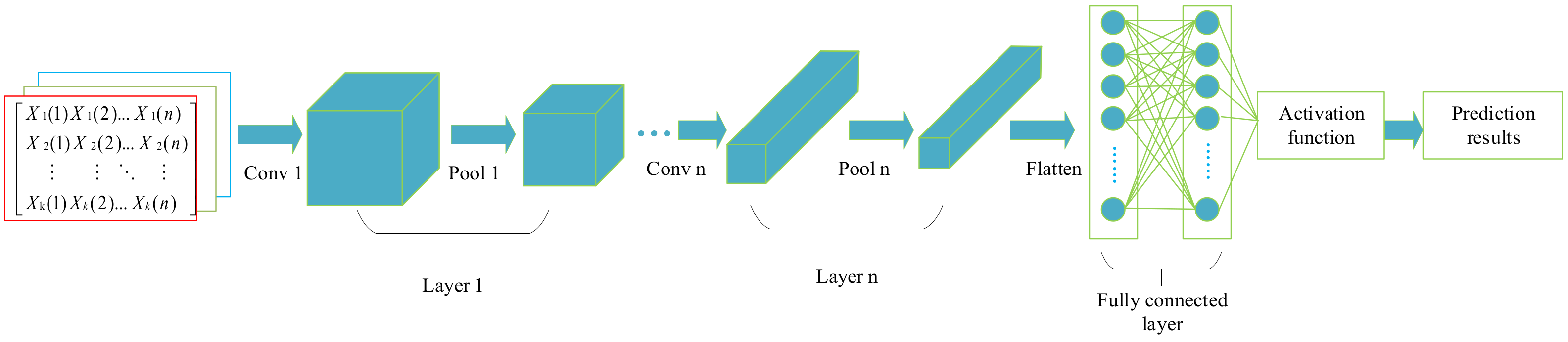
3.2. Convolutional Neural Network

CNNs are widely used in deep learning. They perform higher-level and more abstract processing on original data through local connection and weight sharing, which can automatically extract the internal features of data [39]. A CNN is usually composed of convolutional layers, pooling layers, and fully connected layers, and the structure is shown in Figure 1. As the key to feature extraction, convolution kernels of odd size are commonly used to perform deep convolution operations on data. Then, activation functions such as relu and leaky-relu are used to perform nonlinear mapping on neurons to ignore some secondary features. The pooling layer summarizes the features obtained after the convolution operation and reduces the data dimension through a pooling operation. The fully connected layer is embedded in the bottom layer of the BP neural network to merge the pooled features and calculate the classification or regression prediction results. However, it is difficult for CNNs to learn the relationship between time series. Therefore, it is necessary to integrate a CNN and an RNN for time series prediction.

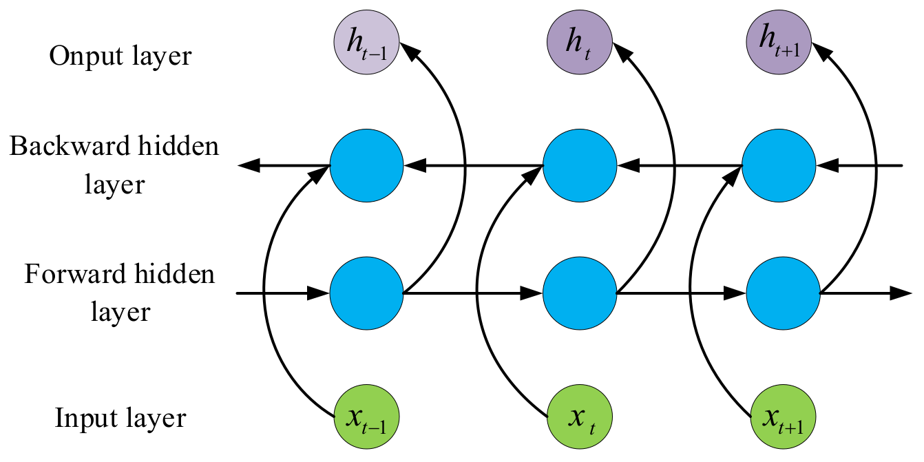
3.3. Bidirectional Gated Neural Network

LSTM is well-suited to deal with time series issues by capturing long-term dependencies. However, the complicated internal composition of the model makes the training time too long. GRUs only contain an update gate and a reset gate, with fewer structural parameters and a faster convergence speed than LSTM [40]. The update gate decides if the historical information of the previous moment is retained in the current status. In addition, the reset gate plays a role in whether the current status is combined with the information from the previous status. Figure 2 shows the structure of a GRU.

In Figure 2, $x_t$ indicates the input values, $h_t$ indicates the output values of the hidden layer, and $u_t$ and $r_t$ indicate the update gate and reset gate, respectively. $\times$ indicates the scalar multiplication of the matrix; $\sigma$ and $\tanh$ indicate the activation function $Sigmoid$ and $\tanh$, respectively; and $1-$ means the information transmitted forward through the link is $1-z_t$. The following formulas calculate the output values of the hidden layer in the GRU network:

$$u_t=\sigma (W^{(u)}{x}_t+U^{(u)}{h}_{t-1})$$

(5)

$$r_t=\sigma (W^{(r)}{x}_t+U^{(r)}{h}_{t-1})$$

(6)

$${\tilde{h}}_t=\tanh (r\times U{h}_{t-1}+W{x}_t)$$

(7)

$$h_t=(1-u)\times \tilde{h}+u_t\times h_{t-1}$$

(8)

In the above formulas, ${\tilde{h}}_t$ indicates the sum of the input $x_t$ and the last hidden status $h_{t-1}$. $U^{(u)}$, $W^{(u)}$, $U^{(r)}$, $W^{(r)}$, $U$, and $W$ are parameter matrices varying with training.

The information is always transmitted forward in the GRU network. However, building energy consumption at a certain time is related to the consumption values in both the historical and future periods. A BiGRU network can simultaneously learn the influence of both past and future factors on current energy consumption, which is more conducive to extracting the deep characteristics of energy consumption data. BiGRU can be regarded as a combination of forward and backward transmitted GRU. The structure is shown in Figure 3. The hidden state $h_t$ at the current moment is determined by three parts: the hidden state $\overrightarrow{h_{t-1}}$ transmitted forward at the moment $t-1$, the hidden state $\overleftarrow{h_{t-1}}$ transmitted backward at the moment $t-1$, and the input $x_t$ at the current moment. The corresponding formula is shown in (9):

$$\left\{\begin{array}{l}\overrightarrow{h_t}=\mathrm{GRU}(x_t,\overrightarrow{h_{t-1}})\\ \overleftarrow{h_t}=\mathrm{GRU}(x_t,\overleftarrow{h_{t-1}})\\ h_t={\alpha }_t\overrightarrow{h_t}+\beta \overleftarrow{h_t}+b_t\end{array}\right.$$

(9)

In the above formula, ${\alpha }_t$ and ${\beta }_t$ are the output weight of the hidden layer corresponding to the forward transmitted GRU and the backward transmitted GRU, respectively. $b_t$ is the bias corresponding to $h_t$.

3.4. Multi-Step Forecasting Strategy

Depending on prediction step size, predictions can be divided into single-step and multi-step forecasts. At present, multi-step forecast mainly includes direct, recursive, direct recursive hybrid, and multi-input multi-output prediction methods. Suppose the input vector is $X_1,X_2,\cdots ,X_N$, the output vector is $Y_1,Y_2,\cdots ,Y_N$, the output step is $M(M>3)$, and the fitting network is $f$. The direct method develops a separate model for each prediction step, which can be expressed in Equation (10):

$$Y_{N+k}=f_k(X_1,X_2,\cdots ,X_N),k\in [1,M]$$

(10)

The recursive multi-step prediction method only needs to establish a model, and the following input of the network comes from the output of the previous step of the network, which can be expressed by Equations (11)–(13):

$$Y_{N+1}=f(X_1,X_2,\cdots ,X_N)$$

(11)

$$Y_{N+2}=f(X_1,X_2,\cdots ,X_N,Y_{N+1})$$

(12)

$$Y_{N+k}=f(X_1,X_2,\cdots ,X_N,Y_{N+1},\cdots ,Y_{N+k-1}),k\in [3,M]$$

(13)

The direct recursive hybrid multi-step prediction method also needs to build a separate model for each prediction step, but each model can use the prediction output value made by the model in the previous time step as the input value, which can be expressed by Equations (14)–(16):

$$Y_{N+1}=f_1(X_1,X_2,\cdots ,X_N)$$

(14)

$$Y_{N+2}=f_2(X_1,X_2,\cdots ,X_{N,}{Y}_{N+1})$$

(15)

$$Y_{N+k}=f_k(X_1,X_2,\cdots ,X_{N,}{Y}_{N+1},Y_{N+k-1}),k\in [3,M]$$

(16)

The multi-input multi-output prediction method only needs to develop a model to output the multi-step prediction values, which can be expressed by Formula (17):

$$(Y_{N+1},Y_{N+2},\cdots ,Y_{N+k})=f(X_1,X_2,\cdots ,X_N)$$

(17)

The direct method needs to establish multiple models simultaneously, which is complicated. Error accumulation exists in the recursive and direct recursive mixed multi-step prediction methods. The multi-input multiple-output prediction method does not have the problem of error accumulation, but the model is more complex and more data are needed to avoid over-fitting. In order to meet the actual forecast demands, this paper adopts the multi-input multi-output prediction method for multi-step prediction.

4. The Hybrid Multi-Step Forecast Model

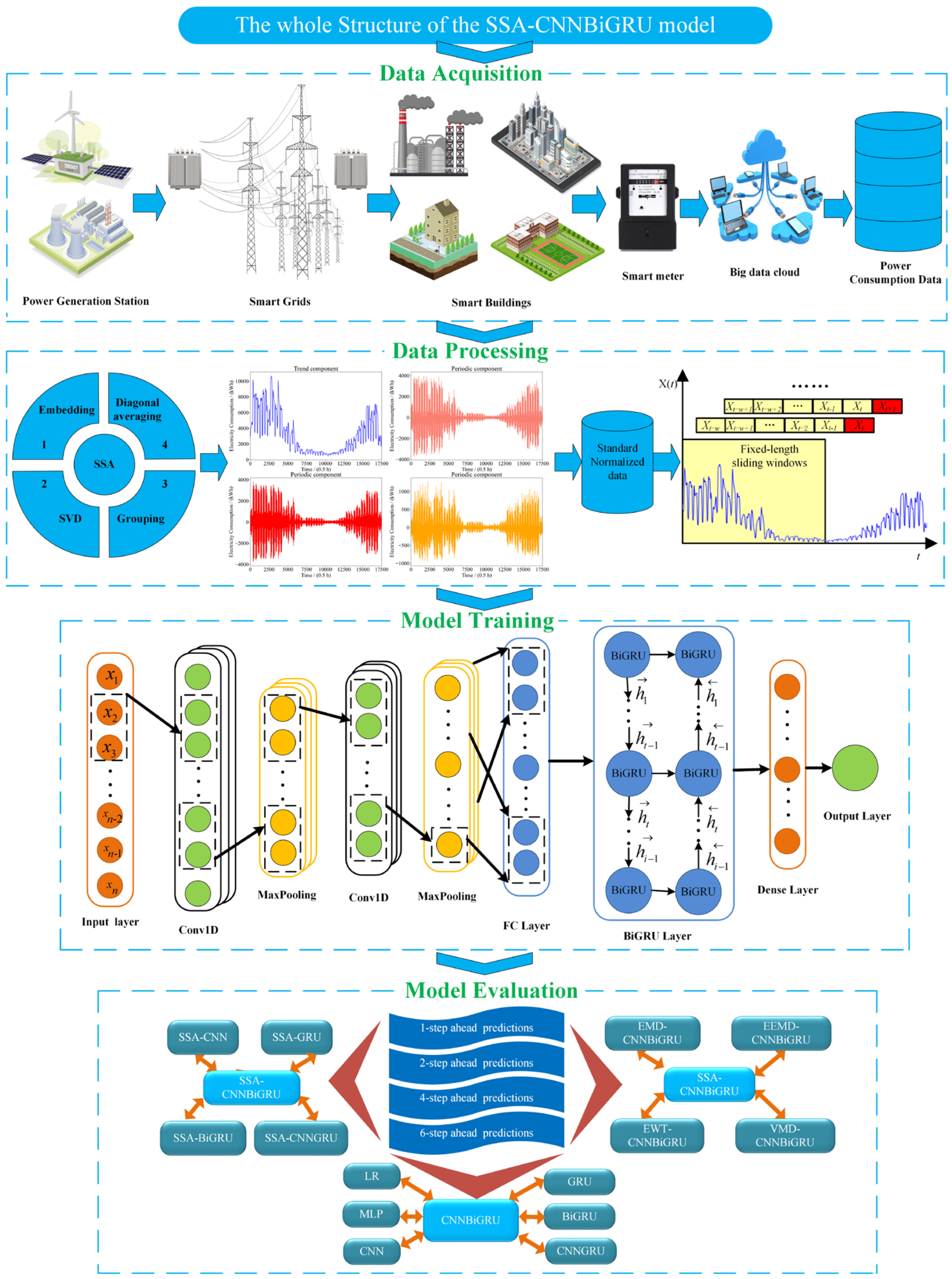
4.1. The Framework of the Proposed Model

This paper proposes a hybrid forecast model based on SSA and CNNBiGRU. The randomness and uncertainty of building energy consumption led to some noise signals in the original consumption data. Initially, SSA was used to remove the noise of the original data and extract the main characteristics of trend and periodic changes. A CNN fully mined the deep features inside the data with a unique structure. A BiGRU network effectively used historical information and future information to model dynamic time series data under the condition of high fluctuation and uncertainty of energy consumption data, which improved learning of the change rule in energy consumption data. Therefore, the CNNBiGRU model predicted each subsequence after SSA noise reduction. The hybrid model proposed in the paper is shown in Figure 4, and the details are as follows:

Step 1: SSA. The original data is decomposed through the SSA method, and the subsequences are divided into one trend component, an $r-1$ periodic component, and an $L-r$ component according to contribution rate and similarity of oscillation frequency.

Step 2: Data standardization. As the fluctuation amplitudes of some component data are still significant, the data are standardized to prevent the network activation function from being over-saturated and to shorten the training time, as shown in Equation (18):

$$X_i^{*}=\frac{X_i-\mu }{\sigma }$$

(18)

where $X_i^{*}$, $X_i$, $\mu$, and $\sigma$ are the standardized value, sample value, mean value, and standard deviation, respectively.

Step 3: Data partition. A sliding window approach is used to convert the noise-removed one-dimensional time series into a shifted two-dimensional array, making the prediction problem a supervised learning problem. Considering that the building energy consumption has a daily periodicity and the data sampling frequency is a half-hour granularity, the sliding window size was set to 48 in the paper. In addition, the training sets and testing sets were divided according to the ratio of 3:1.

Step 4: CNN module. A CNN module plays a role in extracting features of the historical sequences. In this paper, a CNN network framework consisted of two Conv1D layers, two max-pooling layers, and one fully connected layer, and the activation function $\mathrm{Re}lu$ was selected to activate the network. After convolution and pooling operations, the energy consumption data of each subsequence are mapped to the feature space of the hidden layer, then converted and output through the fully connected layer to extract the feature vector. The output feature vector of the CNN layer can be expressed as $H_c$:

$$C_1=f(X\otimes W_1+b_1)=\mathrm{Re}lu(X\otimes W_1+b_1)$$

(19)

$$P_1=\max (C_1)+b_2$$

(20)

$$C_2=f(P\otimes W_2+b_3)=\mathrm{Re}lu(P\otimes W_2+b_3)$$

(21)

$$P_2=\max (C_2)+b_4$$

(22)

$$H_C=f(P_2\times W_3+b_5)=\mathrm{Re}lu(P_2\times W_3+b_5)$$

(23)

In the above formulas, $C_1$ and $C_2$ are output values of the first Conv1D and the second Conv1D, respectively. $P_1$ and $P_2$ are the output values of the first max-pooling layer and the second max-pooling layer, respectively. The weight matrices are represented by $W_1$, $W_2$, and $W_3$. The biases are represented by $b_1$, $b_2$, $b_3$, $b_4$, and $b_5$. $\otimes$ and $\max ()$ are convolution operation and maximum function, respectively. The output of the CNN module is expressed as $H_c=[h_{c1},h_{c2},\cdots ,h_{ct-1},h_{ct},\cdots ,h_{ci-1},h_{ci}]$.

Step 5: BiGRU module. A single layer BiGRU network is established to learn the feature vectors extracted from the CNN module to capture its internal change rules. The output of the BiGRU module is denoted as $h_t$, and the output of step $t$ is represented as:

$$h_t=\mathrm{BiGRU}(H_{C,t-1},H_{C,t}),t\in [1,i]$$

(24)

Step 6: Output module. The output $h_t$ of the BiGRU module is treated as the input of the output module. The output $Y={\left[y_1,y_2,\cdots y_n\right]}^T$ with the prediction step size $n$ is calculated through two layers of dense network, and the formula is as follows:

$$y_t=\mathrm{Re}lu(w_o{s}_t+b_o)$$

(25)

In the formula, $y_t$ represents the predicted value at the moment $t$. $b_o$ and ${\lambda }_o$ are the bias vector and the weight matrix, respectively. In this paper, the $\mathrm{Re}lu$ function is considered as the activation function of the dense layer.

Step 7: Prediction component reconstruction. The prediction results of the trend component $Y_0$ and $n$ group periodic components $Y_i$$(1\le i\le r-1)$ are superimposed to obtain the final predicted value $Y$.

$$Y=Y_0+{\displaystyle \sum _i^{r-1}{Y}_i}$$

(26)

Step 8: Evaluation of prediction results. The performance metrics used in the experiment are $MAE$, $RMSE$, $MAPE$, and $R^2$. The calculation formulas are as shown in

Table 1. Seven evaluation indicators and corresponding calculation formulas.

Index	Definition	Formula
$MAE$	Mean absolute error	$MAE=\frac{1}{n}{\displaystyle \sum _i^n\left|{\widehat{y}}_i-y_i\right|}$
$RMSE$	Root mean square error	$RMSE=\sqrt{\frac{1}{n}{\displaystyle \sum _{i=1}^n{({\widehat{y}}_i-y_i)}^2}}$
$MAPE$	Mean absolute percentage error	$MAPE=\frac{100\%}{n}{\displaystyle \sum _{i=1}^n}\left|({\widehat{y}}_i-y_i)/y_i\right|$
$R^2$	Coefficient of determination	$R^2=1-[{\displaystyle \sum _{i=1}^n}{({\widehat{y}}_i-y_i)}^2-{\displaystyle \sum _{i=1}^n{({\overline{y}}_i-y_i)}^2}]$
$P_{MAE}$	Promoting percentages of mean absolute error	$P_{MAE}=\left|(MA{E}_a-MA{E}_b)/MA{E}_a\right|\times 100$
$P_{RMSE}$	Promoting percentages of root mean square error	$P_{RMSE}=\left|(RMS{E}_a-RMS{E}_b)/RMS{E}_a\right|\times 100$
$P_{MAPE}$	Promoting percentages of mean absolute percentage error	$P_{MAPE}=\left|(MAP{E}_a-MAP{E}_b)/MAP{E}_a\right|\times 100$

. $MSE$ is the mean variance between the forecast value and the actual value, which is always non-negative. $RMSE$ indicates the square root of $MSE$. $MAPE$ reflects the relative relationship between prediction deviation and real value. $R^2$ is used to measure the ratio of the variation of the dependent variable with a value in the range of 0 to 1. The closer the values of $MSE$, $RMSE$, and $MAPE$ are to 0 and the closer the value of $R^2$ is to 1, the better the prediction performance.

In these formulas, $n$ is the sample size. $a$ and $b$ represent the baseline model and the comparison model, respectively. $y_i$, ${\widehat{y}}_i$, and ${\overline{y}}_i$ are the actual value, the forecast value, and the average value at the moment $i$, respectively.

4.2. SSA Data Preprocessing

The experimental datasets came from the energy consumption database of office buildings in the UK. The database recorded electricity and gas consumption of the office buildings from 2 April 2012 to 31 December 2018 with a sampling frequency of half an hour. There were many vacancy values and outliers in the dataset from 2012 to 2017, and the data in 2018 was relatively complete. Therefore, only the data in 2018 was used in this study. The change curves of building energy consumption are shown in Figure 5. The energy consumption of office buildings had the following characteristics: (1) daily periodicity and weekly periodicity, which are consistent with the work and rest rules of office workers; (2) seasonality, which is divided into the heating season, transition season, and cooling season; and (3) randomness, which is affected by uncertain events.

At the same time, in order to fully understand the characteristics of building energy consumption data, the collected datasets are statistically described in

Table 2. Basic statistics of energy consumption data of UK office buildings in 2018.

Consumption Type	Statistic Indices
	Mean (kWh)	Max (kWh)	Min (kWh)	Std	Skew. (Skewness)	Kurt. (Kurtosis)
Electricity	1601.19	4700.72	717.98	774.77	1.10	0.23
Gas	3204.10	19,084.96	269.42	3567.91	2.04	3.76

, and the statistical information mainly involves average value, maximum value, minimum value, standard deviation, skewness, and kurtosis.

In the SSA method, there are two critical parameters to be determined: the length of the embedding window ($L$) and the number of reconstructed subsequences ($r$). Generally, if the original time series is periodic, it is recommended that $L$ is proportional to the periodicity. Considering that the data sampling frequency was 48 points per day and the building energy consumption behavior had a strong daily periodicity, $L$ was set to 48 in all experiments. In addition, the contribution rate of each reconstructed subsequence should be greater than the predetermined threshold, which was set as 0.1% in this paper. The reconstructed subsequence diagram after SSA processing is shown in Figure 6. In Figure 6, the first subsequence of power and natural gas consumption was concentrated on the main energy of the original data, representing the trend component of energy consumption, and the other subsequences oscillated periodically near zero, representing the periodic component of energy consumption. Furthermore, the sum of the contribution rates of the first seven subsequences of power consumption accounted for 99.64% of the original sequence, and the sum of the contribution rates of the first ten subsequences of natural gas consumption accounted for 99.53% of the original sequence, which had the dual effect of retaining a large amount of crucial information and noise reduction.

4.3. Experimental Environment and Network Hyperparameter Setting

The experimental hardware platform was as follows: the CPU was Intel Core i7-8700, the highest frequency was 3.2 GHz, the operating memory was 8 GB, and the Graphics card was Intel HD Graphics 630. Tensorflow 2.0 and Keras 2.3.1 deep learning libraries were used as the backend and Python 3.7.3 software was used for simulation. The hyperparameter configuration of each layer in the CNNBiGRU model is shown in

Table 3. Hyperparameter configuration of each layer in the proposed CNNBiGRU model.

Layer Type	Hyperparameter Configuration
Conv1D	Filters: 16  kernel size: 3  activation: Relu  padding: same
Max-pooling	Pool size: 2  stride: 1  padding: same
Conv1D	Filters: 32  kernel size: 3  activation: Relu  padding: same
Max-pooling	Pool size: 2  stride: 1  padding: same
Dense	Hidden node: 32  activation: Relu
BiGRU	Hidden node: 64  activation: tanh
Dense	Hidden node: 32  activation: Relu
Dense	Hidden node: 1/2/4/6  activation: linear

. Considering the model complexity and data size, the epochs was set to 100, and the batch size was 128. In order to improve the training efficiency and prevent over-fitting of the model, the mechanism of early stopping was adopted, where the tolerance of early stopping was set to 10. The root mean square error was chosen as the loss function, and the model parameters were optimized and adjusted with the Adam (adaptive moment estimation) [41] optimizer. The initial learning rate of the Adam optimizer was set to 0.005 and decayed exponentially by 0.001.

5. Case Studies and Results

In our study, the simulation is mainly composed of three parts. In Section 5.1, to verify the direct prediction effects of the CNNBiGRU model, LR, MLP, CNN, GRU, BiGRU, and CNNGRU models are introduced as comparison methods. LR and MLP use the default parameters in the sklearn library, and the remaining models are consistent with the parameters of each layer in the CNNBiGRU model through desensitization technology. In Section 5.2, after introducing SSA to preprocess the data, SSA-CNN, SSA-GRU, SSA-BiGRU, and SSA-CNNGRU models are compared with the proposed model. In Section 5.3, after preprocessing the original data with the EMD, EEMD, EWT, and VMD decomposition algorithms, the predictions are made based on the CNNBiGRU model, and the models in the paper are compared to investigate effectiveness.

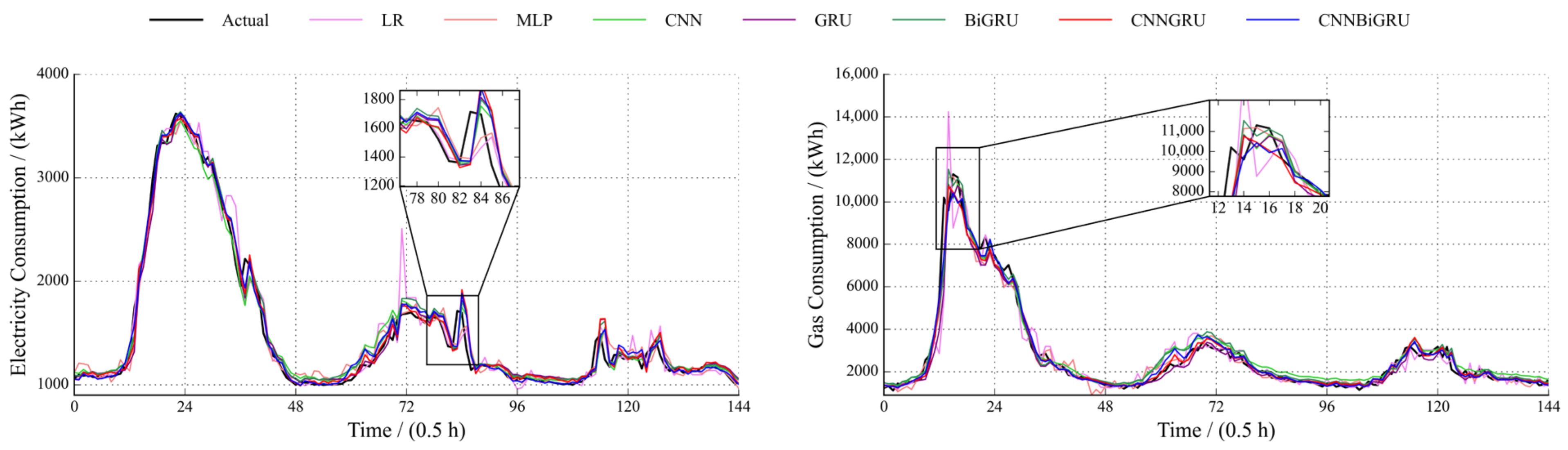
5.1. Comparison of Direct Forecast Results through Different Models

In order to investigate the prediction effectiveness of different models, the prediction error evaluation indicators of seven models with one, two, four, and six steps ahead are given in

Table 4. Comparison of error evaluation indicators for direct multi-step ahead prediction with different models.

Types	Models	MAE (kWh)				RMSE (kWh)				MAPE (%)
		1-Step	2-Step	4-Step	6-Step	1-Step	2-Step	4-Step	6-Step	1-Step	2-Step	4-Step	6-Step
Electricity consumption	LR	120.06	145.24	171.62	198.26	210.62	246.06	288.81	338.95	5.74	6.96	8.18	9.77
	MLP	89.00	119.48	150.14	170.78	149.55	188.62	232.99	266.02	4.62	5.75	7.48	8.43
	CNN	101.11	122.21	178.00	175.30	164.75	201.43	278.31	276.53	5.24	6.22	8.27	9.25
	GRU	87.00	121.16	153.83	172.19	153.54	197.55	242.81	268.86	4.46	6.10	7.33	8.29
	BiGRU	81.51	105.39	140.12	159.43	144.28	175.18	219.34	253.77	4.26	5.32	7.25	8.17
	CNNGRU	81.71	111.69	134.05	160.28	141.51	183.40	214.67	257.08	4.04	5.53	6.62	7.77
	CNNBiGRU	70.06	91.35	116.35	139.09	123.82	151.38	178.67	214.92	3.55	4.65	6.20	7.41
Gas consumption	LR	413.44	492.57	577.35	661.04	694.47	856.17	987.44	1151.58	12.53	14.40	16.92	19.36
	MLP	358.77	456.35	477.81	532.61	531.03	653.25	708.74	815.10	12.59	13.38	14.70	16.31
	CNN	358.09	482.50	474.26	525.21	526.86	702.83	688.95	793.38	13.90	16.40	16.93	17.44
	GRU	363.33	448.09	505.15	529.22	522.63	716.50	800.26	837.83	11.69	12.64	14.13	15.19
	BiGRU	334.96	391.52	425.03	467.70	509.77	647.71	670.21	735.65	10.37	11.70	13.40	14.95
	CNNGRU	301.79	399.83	437.00	490.90	468.57	619.00	693.82	777.07	10.12	13.31	13.82	14.42
	CNNBiGRU	272.20	326.78	386.46	460.75	449.99	515.56	614.03	718.12	8.33	9..99	11.25	13.72

, and the direct forecast results for one step ahead from 5 October to 8 October 2018 are shown in Figure 7. By analyzing the indicators in

Table 5. Prediction error evaluation indicators of different deep neural networks based on the SSA method.

Types	Models	MAE (kWh)				RMSE (kWh)				MAPE (%)
		1-Step	2-Step	4-Step	6-Step	1-Step	2-Step	4-Step	6-Step	1-Step	2-Step	4-Step	6-Step
Electricity consumption	SSA-CNN	37.69	56.95	82.71	94.41	60.48	87.41	134.18	152.30	2.05	3.10	4.00	4.71
	SSA-GRU	34.04	54.12	75.16	99.34	60.49	98.91	130.94	149.43	1.71	2.67	3.75	5.02
	SSA-BiGRU	28.57	44.84	63.69	85.28	53.78	83.89	114.29	134.62	1.39	2.28	3.18	4.35
	SSA-CNNGRU	27.87	37.36	47.17	79.78	50.16	70.36	81.32	122.05	1.27	1.68	2.33	3.97
	SSA-CNNBiGRU	18.52	25.41	38.87	50.96	38.01	49.05	64.41	74.86	0.86	1.21	1.94	2.72
Gas consumption	SSA-CNN	106.34	136.73	184.41	234.30	149.51	186.67	260.81	330.70	3.61	4.85	6.59	8.19
	SSA-GRU	103.08	135.29	193.23	237.25	140.02	196.97	255.59	326.18	3.25	4.63	6.24	7.88
	SSA-BiGRU	92.37	115.18	152.40	227.28	130.57	160.13	225.64	295.99	2.85	3.57	4.68	6.85
	SSA-CNNGRU	84.97	98.23	135.15	183.68	124.59	145.89	212.55	278.61	2.32	3.07	4.29	6.04
	SSA-CNNBiGRU	60.71	78.02	119.33	172.31	93.52	115.36	174.24	247.75	1.78	2.44	3.86	5.67

and the prediction curve in Figure 6, the following can be observed:

(1) The prediction error evaluation indicators of the CNNBiGRU model had a certain degree of decline compared with the other four prediction models. In the one-step ahead prediction of building power consumption, the MAPE of the CNNBiGRU model was 38.2%, 23.2%, 32.25%, 20.10%, 16.17%, and 12.13% lower than that of the LR, MLP, CNN, GRU, BiGRU, and CNNGRU models, respectively. This indicates that a CNN extracts the inherent deep features of the original building energy consumption data, and then inputs them into the BiGRU network for prediction, which can effectively improve the prediction accuracy of the model;

(2) Building energy consumption had apparent daily periodicity with a higher consumption value for weekdays and a lower consumption value for weekends. Power consumption peaked at noon, while natural gas consumption peaked in the morning. This phenomenon reflects the energy consumption behavior of a typical office building on workdays and non-workdays. Compared with the other six models, the prediction curve of the CNNBiGRU model was more consistent with the original time series of energy consumption, and the prediction effect was better for smooth data. However, an apparent lag phenomenon near the extreme point indicates that direct prediction cannot effectively identify the mutation of energy consumption behavior;

(3) With the increase in the size of prediction steps, the prediction error evaluation indicators of the prediction models increased by varying degrees, which shows that these models are sensitive to the prediction step size and cannot meet the prediction accuracy requirements in multi-step prediction scenarios. Therefore, these models are not suitable for the multi-step ahead prediction of building energy consumption.

5.2. Comparison of Forecast Results of Different Models under Singular Spectrum Decomposition

In order to verify the forecast performance improvement of the models after the integrated SSA method, the prediction error evaluation indicators of five deep neural networks after the integrated SSA method with one, two, four, and six steps ahead are given in Table 5.

Table 6. Optimization percentage of integrated SSA method for prediction error evaluation indicators under one-step ahead prediction.

Models	Electricity Consumption			Gas Consumption
	${\mathit{P}}_{\mathit{M}\mathit{A}\mathit{E}}$/%	${\mathit{P}}_{\mathit{R}\mathit{M}\mathit{S}\mathit{E}}$/%	${\mathit{P}}_{\mathit{M}\mathit{A}\mathit{P}\mathit{E}}$/%	${\mathit{P}}_{\mathit{M}\mathit{A}\mathit{E}}$/%	${\mathit{P}}_{\mathit{R}\mathit{M}\mathit{S}\mathit{E}}$/%	${\mathit{P}}_{\mathit{M}\mathit{A}\mathit{P}\mathit{E}}$/%
CNN	62.72	63.29	60.88	70.30	71.22	74.03
GRU	60.87	60.60	61.66	71.63	73.21	72.20
BiGRU	64.95	62.73	67.37	72.42	74.39	72.51
CNNGRU	65.89	64.55	68.56	71.84	73.41	77.07
CNNBiGRU	76.85	69.30	75.77	77.70	79.22	78.63

shows the optimization percentage of error evaluation indicators when the models make one-step ahead prediction after integrating the SSA method. Figure 8 shows the comparison of the one-step ahead forecast results for the CNNBiGRU model before and after integrating the SSA method. Through the analysis of the information in the figure and table, the following can be observed:

(1) Compared with the individual deep neural network model, the forecast precision of the integrated model based on the SSA method was greatly improved. In one-step ahead prediction of power consumption, compared with the CNNBiGRU model, the optimization percentages of the error evaluation indicators of the SSA-CNNBiGRU model were 76.85%, 69.30%, and 75.77%, and the improvement was clear. It can be inferred that the higher the forecast precision of the original model, the more pronounced the improvement after integrating the SSA algorithm;

(2) After integrating the SSA method, the CNNBiGRU model had a stronger ability to capture the peaks and valleys in the original energy consumption time series, and the prediction lag phenomenon near the extreme point data was effectively alleviated. The results showed that the SSA method decomposed the original building energy consumption data to extract the trend and periodic components, and then the neural network prediction model was used to predict, which effectively identified the randomness and uncertainty of building energy consumption behavior to improve the prediction accuracy.

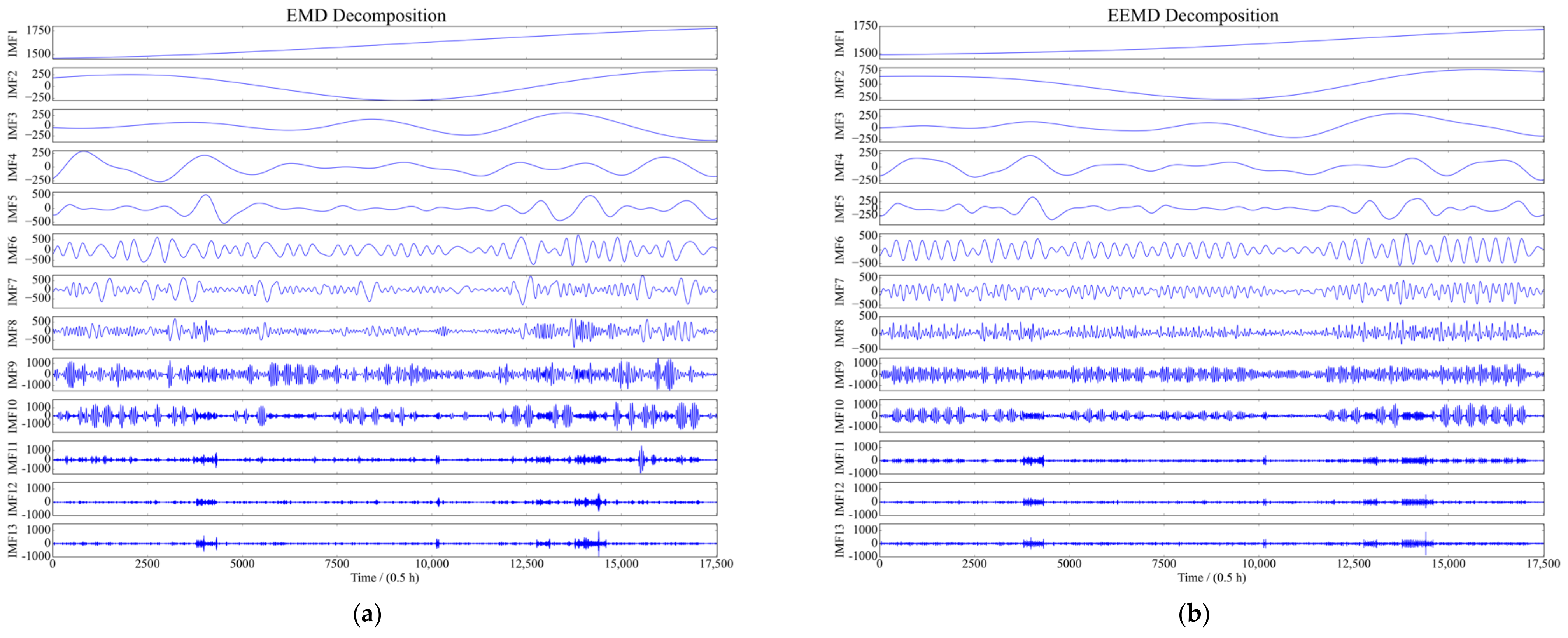
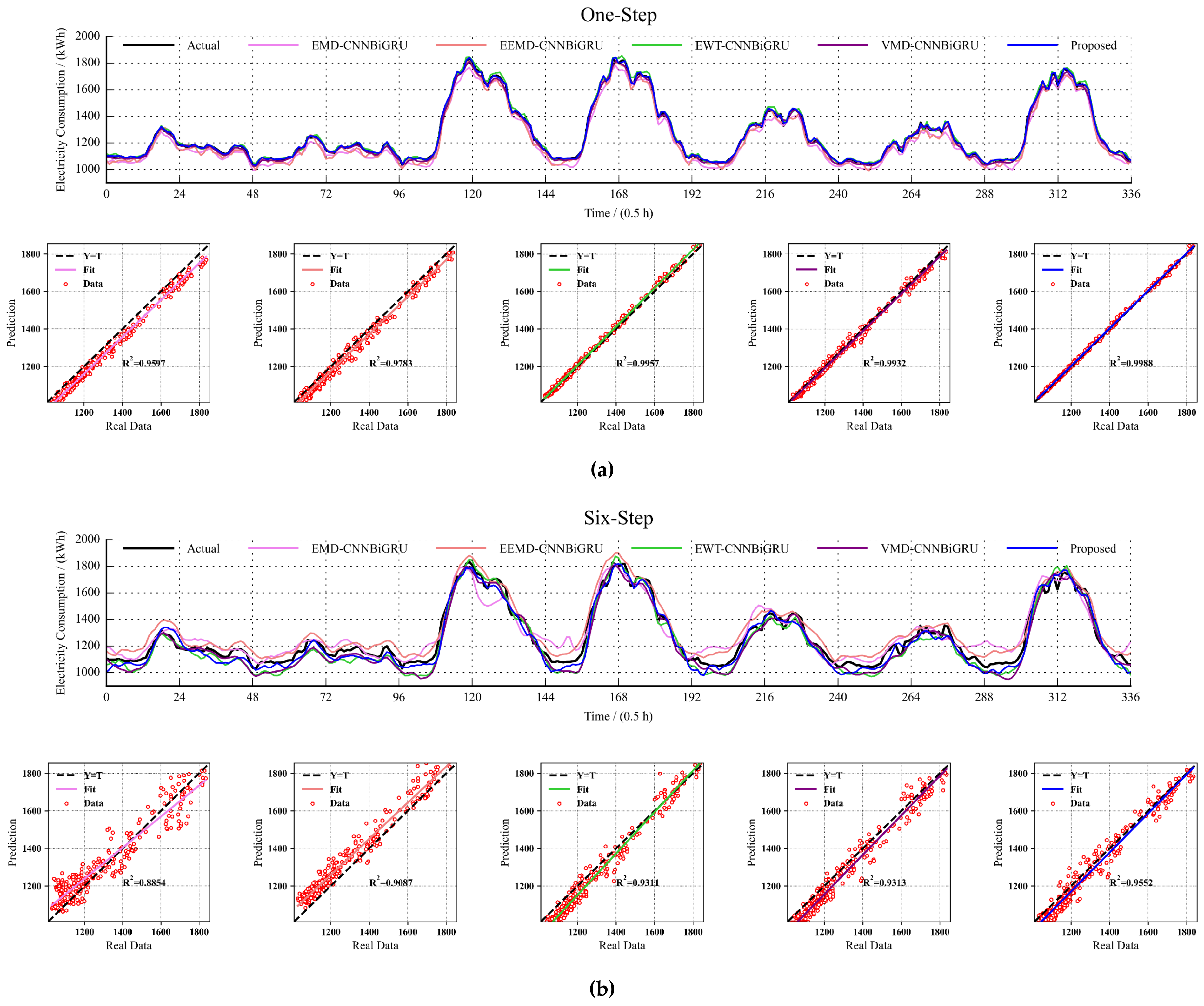
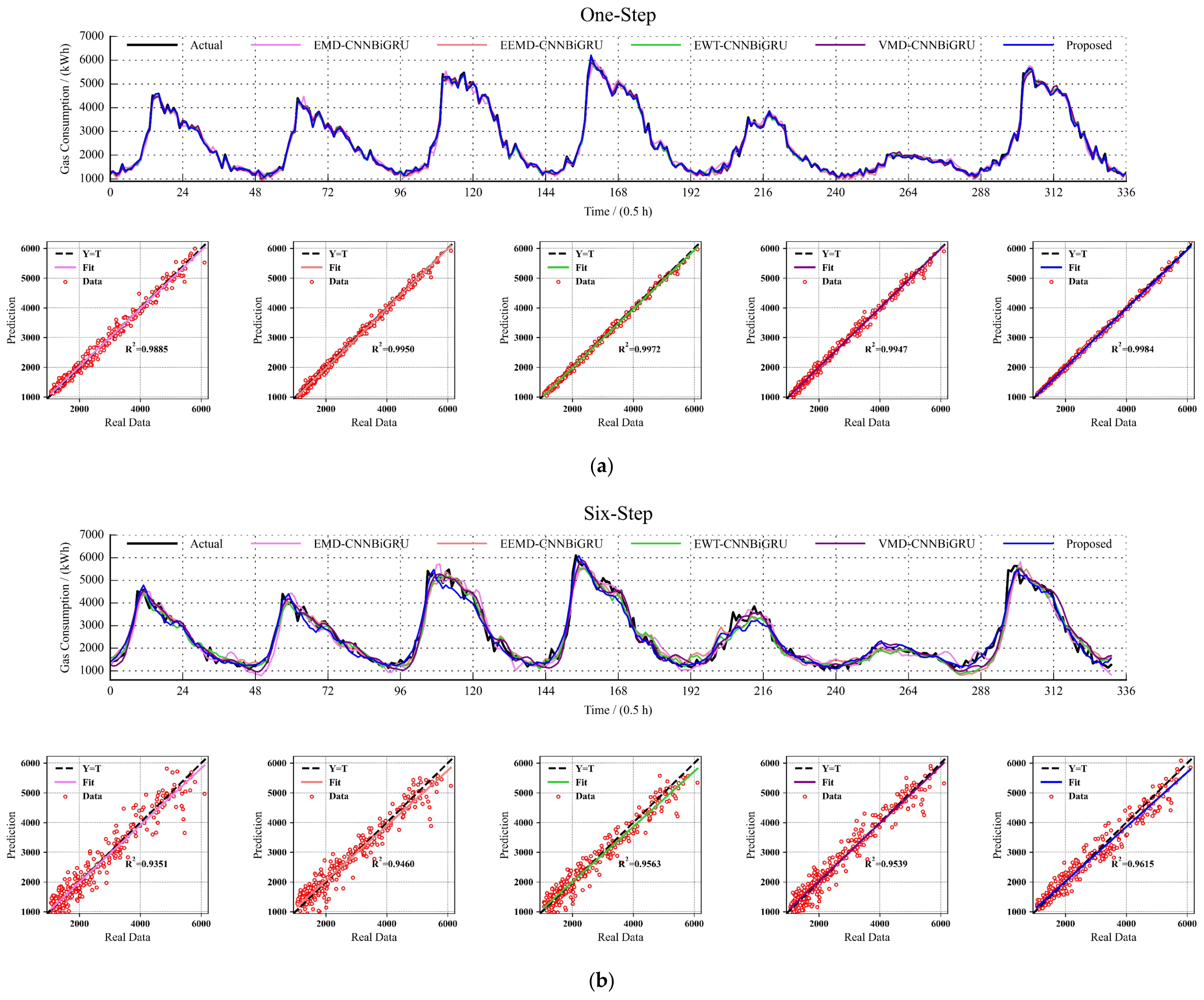
5.3. Comparison of Forecast Results under Different Decomposition Algorithms

In this section, the CNNBiGRU networks optimized by EMD, EEMD, EWT, and VMD algorithms are compared with the proposed model. In the power consumption data, the number of EMD and EEMD adaptive decomposition layers was 13, and the number of EWT and VMD decomposition levels was set to 7. In the natural gas consumption data, the number of EMD and EEMD adaptive decomposition layers was 14, and the number of EWT and VMD decomposition layers was set to 10. Taking building power consumption data as an example, Figure 9 shows the subsequence diagrams obtained by applying these four decomposition algorithms. Figure 9a,b show the results of 13 subsequences after EMD and EEMD adaptive decomposition, respectively. The amplitudes of the IMF1 component varied from 1500 to 1700 kWh, which concentrated on most of the energy from the original sequence. The amplitudes of the IMF2~IMF13 components varied from −1000 to 1000 kWh, which included the main components of the original data. Figure 9c shows the results of seven subsequences after EWT decomposition of the data. The amplitude of the IMF1 component varied from 1000 to 4000 kWh, which contained more detailed components than the IMF1 component for EMD and EEMD. Figure 9d shows the results of seven subsequences after VMD decomposition of the data. The IMF1 component had the largest amplitude and occupied most of the original sequence, reflecting the main changes in the original signal.

The multi-steps ahead prediction performance evaluation indicators are shown in

Table 7. Comparison of prediction error evaluation indexes based on the CNNBiGRU model with different decomposition methods.

Types	Models	MAE (kWh)				RMSE (kWh)				MAPE (%)
		1-Step	2-Step	4-Step	6-Step	1-Step	2-Step	4-Step	6-Step	1-Step	2-Step	4-Step	6-Step
Electricity consumption	EMD-CNNBiGRU	51.76	59.30	73.55	98.33	78.97	92.04	114.78	157.24	2.85	3.16	4.00	5.43
	EEMD-CNNBiGRU	40.25	50.33	63.12	81.60	54.31	68.74	87.30	111.75	2.26	3.04	3.75	5.00
	EWT-CNNBiGRU	29.03	42.33	50.59	64.45	43.45	58.10	73.83	92.39	1.46	2.29	2.63	3.44
	VMD-CNNBiGRU	35.84	42.70	56.66	69.83	55.46	68.00	87.49	103.14	1.88	2.24	2.96	3.69
	SSA-CNNBiGRU	18.52	25.41	38.87	50.96	38.01	49.05	64.41	74.86	0.86	1.21	1.94	2.72
Gas consumption	EMD-CNNBiGRU	139.77	186.33	254.38	310.73	204.47	278.29	381.10	443.92	5.04	6.67	9.37	11.83
	EEMD-CNNBiGRU	118.56	127.31	181.13	236.61	159.43	175.42	258.87	332.68	4.45	4.82	6.60	8.82
	EWT-CNNBiGRU	76.84	91.44	135.77	180.54	105.79	122.88	187.76	252.64	2.98	3.51	5.05	6.71
	VMD-CNNBiGRU	103.94	111.57	158.78	190.49	142.72	156.61	219.46	268.57	3.80	4.10	5.88	6.79
	SSA-CNNBiGRU	60.71	78.02	119..33	172.31	93.52	115.36	174.24	247.75	1.78	2.44	3.86	5.67

. Since the multi-step ahead prediction results have the same overall error performance, only the one-step ahead prediction results of building power consumption were analyzed. From Table 7, the following observations can be made:

(1) The MAPE optimization percentages of the SSA algorithm for the EMD, EEMD, EWT, and VMD algorithms were 69.8%, 61.9%, 41.1%, and 54.3%, respectively. It can be shown that the SSA method is a suitable feature extractor that separates the trend, periodic, and noise components from the original sequence, which is helpful to improve the prediction performance of the model;

(2) Compared with the EMD algorithm, the optimization percentages of the MAE, RMSE, and MAPE values for the EEMD algorithm were 22.2%, 31.2%, and 20.7%, respectively. This can be explained because EEMD utilizes the statistical characteristics of white noise to eliminate the modal aliasing problem of EMD, which improves the stability of each subsequence after decomposition. However, EEMD cannot eliminate the shortcomings of EMD. Therefore, EEMD has limited improvement on the final forecast precision of the CNNBiGRU model;

(3) Compared with the EMD algorithm, the optimization percentages of the MAE, RMSE, and MAPE values of the EWT algorithm were 43.9%, 45.0%, and 48.8%, respectively. This can be explained because EWT combines the advantages of both WT and EMD to adaptively generate wavelet basis functions, which solves the problems of the theory of the EMD algorithm being insufficient and the convergence conditions being challenging to define;

(4) Compared with the EMD algorithm, the optimization percentages of the MAE, RMSE, and MAPE values of the VMD algorithm were 30.8%, 29.8%, and 34.0%, respectively. It can be observed that the forecast precision of the VMD algorithm was superior to EMD and EEMD. This can be explained because the VMD algorithm can moderate the influence of data volatility and nonlinearity on the prediction results and solve the problem of noise residue in EMD and EEMD algorithms.

Figure 10 and Figure 11 demonstrate the forecast results of the CNNBiGRU model optimized by five decomposition algorithms from 25 December to 31 December 2018, which represented the energy consumption behavior of office buildings during holiday periods. The following observations can be made through analyzing the information in the figures:

(1) The building energy consumption was low and the change was relatively flat during Christmas (25 December), which was related to the data selected from British office buildings;

(2) Among all the prediction results, for one-step ahead and six-steps ahead, the model proposed had the best prediction effects, and the changing trend of its prediction results was the same as the changing trend of the actual value. The $R^2$ value was the closest to 1, and the fitting degree was the highest;

(3) With the increase of prediction steps, the precision of the five decomposition prediction models decreased. Especially for EMD-CNNBiGRU, when the size of the prediction step reached six, the model accuracy dropped sharply, causing the prediction curve to no longer meet the accuracy requirements of the prediction model.

6. Conclusions and Future Works

Our paper proposes a SSA-CNNBiGRU model for short-term forecasting of building energy consumption. In the proposed model, an SSA method is used to decompose and denoise the original building energy consumption data, and the CNNBiGRU model aims to forecast the main components of the building energy consumption series. The simulation results under three scenarios showed that: (1) the CNNBiGRU model had excellent performances for automatic feature extraction and processing time series dependence, which effectively increased the forecast precision. (2) The proposed SSA-CNNBiGRU model achieved satisfactory results for short-term prediction of building energy consumption, not only effectively capturing the changes of peaks and valleys of building energy consumption, but also effectively identifying the mutation of building energy consumption behavior to alleviate the hysteresis phenomenon of extreme point data prediction. (3) SSA was an ideal decomposition algorithm, separating the trend, periodic, and noise components from the original building energy consumption series. Moreover, the proposed model effectively alleviated the accuracy reduction in multi-step prediction and met building energy consumption requirements.

Although the SSA-CNNBiGRU model achieved satisfactory results in building energy consumption forecasting, the lack of consideration of external factors on building energy consumption and the parameters of the proposed model are the main limitations of this paper. Future research will focus on three directions: (1) Considering that building energy consumption is affected by multiple factors, such as temperature and calendar, we should try to build a more reasonable model in a multivariable scenario. (2) The prediction performances of deep learning methods are often affected by hyperparameter, so it is necessary to use an optimization algorithm to optimize the hyperparameter in the deep neural network. (3) We will use this model to make short-term predictions for the energy consumption of individual residents with more randomness to further validate the practicability of the proposed model.

References

1. Aversa, P.; Donatelli, A.; Piccoli, G.; Luprano, V.A.M. Improved Thermal Transmittance Measurement with HFM Technique on Building Envelopes in the Mediterranean Area. Sel. Sci. Pap.-J. Civ. Eng. 2016, 11, 39–52. [Google Scholar] [CrossRef] [Green Version]
2. Runge, J.; Zmeureanu, R. A Review of Deep Learning Techniques for Forecasting Energy Use in Buildings. Energies 2021, 14, 608. [Google Scholar] [CrossRef]
3. Bourdeau, M.; Zhai, X.Q.; Nefzaoui, E.; Guo, X.; Chatellier, P. Modeling and forecasting building energy consumption: A review of data-driven techniques. Sustain. Cities Soc. 2019, 48, 101533. [Google Scholar] [CrossRef]
4. López Gómez, J.; Troncoso Pastoriza, F.; Fariña, E.A.; Oller, P.E.; Álvarez, E.G. Use of a numerical weather prediction model as a meteorological source for the estimation of heating demand in building thermal simulations. Sustain. Cities Soc. 2020, 62, 102403. [Google Scholar] [CrossRef]
5. Li, Y.; Tong, Z.; Tong, S.; Westerdahl, D. A data-driven interval forecasting model for building energy prediction using attention-based LSTM and fuzzy information granulation. Sustain. Cities Soc. 2022, 76, 103481. [Google Scholar] [CrossRef]
6. Mariano-Hernández, D.; Hernández-Callejo, L.; Solís, M.; Zorita-Lamadrid, A.; Duque-Perez, O.; Gonzalez-Morales, L.; Santos-García, F. A Data-Driven Forecasting Strategy to Predict Continuous Hourly Energy Demand in Smart Buildings. Appl. Sci. 2021, 11, 7886. [Google Scholar] [CrossRef]
7. Fang, X.; Gong, G.; Li, G.; Chun, L.; Li, W.; Peng, P. A hybrid deep transfer learning strategy for short term cross-building energy prediction. Energy 2021, 215, 119208. [Google Scholar] [CrossRef]
8. Calvillo, C.F.; Sánchez-Miralles, A.; Villar, J. Energy management and planning in smart cities. Renew. Sustain. Energy Rev. 2016, 55, 273–287. [Google Scholar] [CrossRef] [Green Version]
9. Lü, X.; Lu, T.; Kibert, C.J.; Viljanen, M. Modeling and forecasting energy consumption for heterogeneous buildings using a physical–statistical approach. Appl. Energy 2015, 144, 261–275. [Google Scholar] [CrossRef]
10. Kong, W.; Dong, Z.Y.; Jia, Y.; Hill, D.J.; Xu, Y.; Zhang, Y. Short-Term Residential Load Forecasting Based on LSTM Recurrent Neural Network. IEEE Trans. Smart Grid 2019, 10, 841–851. [Google Scholar] [CrossRef]
11. Deb, C.; Zhang, F.; Yang, J.; Lee, S.E.; Shah, K.W. A review on time series forecasting techniques for building energy consumption. Renew. Sustain. Energy Rev. 2017, 74, 902–924. [Google Scholar] [CrossRef]
12. Hao, Z.; Liu, G.; Zhang, H. Correlation filter-based visual tracking via adaptive weighted CNN features fusion. IET Image Process. 2018, 12, 1423–1431. [Google Scholar] [CrossRef]
13. Hochreiter, S.S.J. Long Short-Term Memory. Neural Comput. 1997, 9, 1735–1780. [Google Scholar] [CrossRef] [PubMed]
14. Cho, K.; van Merriënboer, B.; Gulcehre, C.; Bahdanau, D.; Bougares, F.; Schwenk, H.; Bengio, Y. Learning Phrase Representations using RNN Encoder-Decoder for Statistical Machine Translation. arXiv 2014, arXiv:1406.1078. [Google Scholar]
15. Zhang, H.; Yang, Y.; Zhang, Y.; He, Z.; Yuan, W.; Yang, Y.; Qiu, W.; Li, L. A combined model based on SSA, neural networks, and LSSVM for short-term electric load and price forecasting. Neural Comput. Appl. 2021, 33, 773–788. [Google Scholar] [CrossRef]
16. Afshar, K.; Bigdeli, N. Data analysis and short term load forecasting in Iran electricity market using singular spectral analysis (SSA). Energy 2011, 36, 2620–2627. [Google Scholar] [CrossRef]
17. An, L.; Hao, Y.; Yeh, T.-C.J.; Liu, Y.; Liu, W.; Zhang, B. Simulation of karst spring discharge using a combination of time–frequency analysis methods and long short-term memory neural networks. J. Hydrol. 2020, 589, 125320. [Google Scholar] [CrossRef]
18. Mi, X.; Zhao, S. Wind speed prediction based on singular spectrum analysis and neural network structural learning. Energy Convers. Manag. 2020, 216, 112956. [Google Scholar] [CrossRef]
19. Wang, C.; Zhang, H.; Ma, P. Wind power forecasting based on singular spectrum analysis and a new hybrid Laguerre neural network. Appl. Energy 2020, 259, 114139. [Google Scholar] [CrossRef]
20. Liu, H.; Mi, X.; Li, Y.; Duan, Z.; Xu, Y. Smart wind speed deep learning based multi-step forecasting model using singular spectrum analysis, convolutional Gated Recurrent Unit network and Support Vector Regression. Renew. Energy 2019, 143, 842–854. [Google Scholar] [CrossRef]
21. Massana, J.; Pous, C.; Burgas, L.; Melendez, J.; Colomer, J. Short-term load forecasting in a non-residential building contrasting models and attributes. Energy Build. 2015, 92, 322–330. [Google Scholar] [CrossRef] [Green Version]
22. Blázquez-García, A.; Conde, A.; Milo, A.; Sánchez, R.; Barrio, I. Short-term office building elevator energy consumption forecast using SARIMA. J. Build. Perform. Simul. 2020, 13, 69–78. [Google Scholar] [CrossRef]
23. Zhang, F.; Deb, C.; Lee, S.E.; Yang, J.; Shah, K.W. Time series forecasting for building energy consumption using weighted Support Vector Regression with differential evolution optimization technique. Energy Build. 2016, 126, 94–103. [Google Scholar] [CrossRef]
24. Culaba, A.B.; Del Rosario, A.J.; Ubando, A.T.; Chang, J.S. Machine learning-based energy consumption clustering and forecasting for mixed-use buildings. Int. J. Energy Res. 2020, 44, 9659–9673. [Google Scholar] [CrossRef]
25. Wang, Z.; Wang, Y.; Zeng, R.; Srinivasan, R.; Ahrentzen, S. Random Forest based hourly building energy prediction. Energy Build. 2018, 171, 11–25. [Google Scholar] [CrossRef]
26. Naji, S.; Keivani, A.; Shamshirband, S.; Alengaram, U.J.; Jumaat, M.Z.; Mansor, Z.; Lee, M. Estimating building energy consumption using extreme learning machine method. Energy 2016, 97, 506–516. [Google Scholar] [CrossRef]
27. Olu-Ajayi, R.; Alaka, H.; Sulaimon, I.; Sunmola, F.; Ajayi, S. Building energy consumption prediction for residential buildings using deep learning and other machine learning techniques. J. Build. Eng. 2022, 45, 103406. [Google Scholar] [CrossRef]
28. Fan, C.; Sun, Y.; Zhao, Y.; Song, M.; Wang, J. Deep learning-based feature engineering methods for improved building energy prediction. Appl. Energy 2019, 240, 35–45. [Google Scholar] [CrossRef]
29. Wen, L.; Zhou, K.; Yang, S. Load demand forecasting of residential buildings using a deep learning model. Electr. Power Syst. Res. 2020, 179, 106073. [Google Scholar] [CrossRef]
30. Khan, Z.A.; Hussain, T.; Ullah, A.; Rho, S.; Lee, M.; Baik, S.W. Towards Efficient Electricity Forecasting in Residential and Commercial Buildings: A Novel Hybrid CNN with a LSTM-AE based Framework. Sensors 2020, 20, 1399. [Google Scholar] [CrossRef] [Green Version]
31. Somu, N.; Raman MR, G.; Ramamritham, K. A deep learning framework for building energy consumption forecast. Renew. Sustain. Energy Rev. 2021, 137, 110591. [Google Scholar] [CrossRef]
32. Eseye, A.T.; Lehtonen, M. Short-Term Forecasting of Heat Demand of Buildings for Efficient and Optimal Energy Management Based on Integrated Machine Learning Models. IEEE Trans. Ind. Inform. 2020, 16, 7743–7755. [Google Scholar] [CrossRef]
33. Sun, H.; Zhai, W.; Wang, Y.; Yin, L.; Zhou, F. Privileged information-driven random network based non-iterative integration model for building energy consumption prediction. Appl. Soft Comput. 2021, 108, 107438. [Google Scholar] [CrossRef]
34. Gao, X.; Qi, C.; Xue, G.; Song, J.; Zhang, Y.; Yu, S.-A. Forecasting the Heat Load of Residential Buildings with Heat Metering Based on CEEMDAN-SVR. Energies 2020, 13, 6079. [Google Scholar] [CrossRef]
35. Kim, S.H.; Lee, G.; Kwon, G.-Y.; Kim, D.-I.; Shin, Y.-J. Deep Learning Based on Multi-Decomposition for Short-Term Load Forecasting. Energies 2018, 11, 3433. [Google Scholar] [CrossRef] [Green Version]
36. Chen, Y.; Tan, H. Short-term prediction of electric demand in building sector via hybrid support vector regression. Appl. Energy 2017, 204, 1363–1374. [Google Scholar] [CrossRef]
37. Zhang, L.; Alahmad, M.; Wen, J. Comparison of time-frequency-analysis techniques applied in building energy data noise cancellation for building load forecasting: A real-building case study. Energy Build. 2021, 231, 110592. [Google Scholar] [CrossRef]
38. Yuan, Z.; Wang, W.; Wang, H.; Mizzi, S. Combination of cuckoo search and wavelet neural network for midterm building energy forecast. Energy 2020, 202, 117728. [Google Scholar] [CrossRef]
39. Kuo, P.; Huang, C. A High Precision Artificial Neural Networks Model for Short-Term Energy Load Forecasting. Energies 2018, 11, 213. [Google Scholar] [CrossRef] [Green Version]
40. Wang, Y.; Liao, W.; Chang, Y. Gated Recurrent Unit Network-Based Short-Term Photovoltaic Forecasting. Energies 2018, 11, 2163. [Google Scholar] [CrossRef] [Green Version]
41. Kingma, D.P.; Ba, J. Adam: A Method for Stochastic Optimization. arXiv 2014, arXiv:1412.6980. [Google Scholar]
Figure 1. Structure diagram of a CNN.
Energies 15 01743 g001
Figure 2. Structure diagram of a GRU.
Energies 15 01743 g002
Figure 3. Structure diagram of a BiGRU network.
Energies 15 01743 g003
Figure 4. The overall structure of the proposed SSA-CNNBiGRU model.
Energies 15 01743 g004
Figure 5. Half-hour resolution energy consumption curves for UK office buildings in 2018.
Energies 15 01743 g005
Figure 6. The first seven subsequences of power consumption and the first ten subsequences of natural gas consumption after SSA preprocessing.
Energies 15 01743 g006
Figure 7. Comparison of one-step ahead direct forecast results of seven models.
Energies 15 01743 g007
Figure 8. Comparison of one-step ahead prediction results for the SSA-CNNBiGRU and CNNBiGRU models.
Energies 15 01743 g008
Figure 9. Decomposition results of building power consumption data with different decomposition algorithms.
Energies 15 01743 g009aEnergies 15 01743 g009b
Figure 10. Multi-step ahead building power consumption prediction results from different decomposition algorithms: (a) one-step and (b) six-step.
Energies 15 01743 g010
Figure 11. Multi-step ahead building gas consumption prediction results for different decomposition algorithms: (a) one-step and (b) six-step.
Energies 15 01743 g011