Intelligent Power Distribution Restoration Based on a Multi-Objective Bacterial Foraging Optimization Algorithm

Abstract

The importance of power in society is indisputable. Virtually all economic activities depend on electricity. The electric power systems are complex, and move studies in different areas are motivated to make them more efficient and solve their operational problems. The smart grids emerged from this approach and aimed to improve the current systems and integrate electric power using alternative and renewable sources. Restoration techniques of these networks are being developed to reduce the impacts caused by the usual power supply interruptions due to failures in the distribution networks. This paper presents the development and evaluation of the performance of a multi-objective version of the Bacterial Foraging Optimization Algorithm for finding the minor handling switches that maximize the number of buses served, keeping the configuration radial system and within the limits of current in the conductors and bus voltage. An electrical system model was created, and routines were implemented for the network verification, which was used as a function of the Multi-Objective Bacterial Foraging Optimization Hybrid Algorithm. The proposed method has been applied in two distribution systems with 70 buses and 201 buses, respectively, and the algorithm’s effectiveness to solve the restoration problem is discussed.

1. Introduction

Electrical power systems exist to produce and deliver electricity to various consumers. These systems move studies in different areas to make them more efficient and solve their operational problems. Telecommunications technologies and computational tools have been implemented in other applications, such as smart power grids, known as smart grids, which emerged from the approximation of these areas and aimed to improve current electrical systems [1]. Smart grids are equipped with monitoring systems and remote operation of your equipment. These networks allow the supply of energy in a controlled and intelligent way, analyzing, among other factors, the consumption patterns of users, and can integrate ways of generating electricity through alternative, renewable sources [2] and electrical and gas storage [3].

Damage to the infrastructure of electrical networks, caused by storms, traffic accidents, vandalism, among other factors, is widespread and can cause interruptions in the electricity supply. In 2012, about 8 million people were left without electricity during Hurricane Sandy’s passage in the United States. The country’s economy is estimated to lose more than $150 billion a year due to interruptions in the electricity supply [4].

Techniques have been developed to reduce the impacts caused by these interruptions. These techniques try to recover the power distribution system, aiming to minimize the time required to restore supply and reduce the number of people affected [5]. Among them, computational intelligence optimization techniques, such as bio-inspired techniques [6], have been widely applied to design optimal plants, find the best configuration of restore switches and select the optimal sequence of operation of these switches.

With the expansion of new smart grids technologies for monitoring and remote performance in networks, efficient computational techniques will be increasingly important. The process known as self-healing has been studied to make intelligent power grids capable of recovering from faults in a fully autonomous way.

Current equipment effectively detects failures, and some initiatives can already suggest the actions needed to restore networks. However, the role of operators is still required to implement the solutions [7]. In addition, restoration plants need to be constantly updated. Due to the growth of cities and increased energy consumption, substations become overloaded and quickly become obsolete.

The restoration problem in the distribution network was initially treated by numerical methods, using mathematical programmings like mixed-integer linear optimization [8] or second-order optimization [9], or mathematical morphology [10]. However, the quality of the solutions found by these methods depends on the search space. In multi-modal search spaces or nonconvex search spaces, these methods can not have a good solution because it is impossible to produce tunneling.

With the advent of intelligent meta-heuristics techniques, some solutions have been developed to optimize restoring these networks. Optimization techniques such as PSO (particle swarm optimization) [11] and GA (genetic algorithm) [12] have been widely applied to design optimal plants, find the best positioning of restore switches and select the optimal sequence of operation of these switches. References [13,14,15] present examples of applications of PSO to provide restoration solutions for distribution systems, while references [16,17,18] deliver these solutions using GA techniques.

All meta-heuristic techniques are stochastic algorithms, meaning they involve random processes. In these algorithms, each initial condition and set of initial parameters produce a given solution. For this reason, a suitable adjustment of the initial parameters is necessary to avoid problems, like local minimums or premature convergence. And more, the algorithms must be executed several times, comparing their responses and selecting the best solution.

This paper proposes another intelligent meta-heuristic approach using the Multi-Objective Bacteria Culture Optimization Hybrid Algorithm (MOBCOHA) to solve the restoration problem. This new algorithm merges ideas shown in two references [19,20]. Then, given a system that failed, the proposed program performs power flow calculations on the network to find a minimum amount of switch opening and closing operations that result in a combination that maximizes the number of loads served.

This paper is structured as follows. The proposed MOBCOHA is presented with their most essential concepts in the second section. After, in the third section, the details of the development of the proposed approach are given. This section also includes information about the techniques and algorithms used. In Section 4, the results of some experiments compared to other algorithms are shown in an 11 kV radial distribution network used in many published studies and a 201-buses distribution network. Finally, Section 5 is presented the conclusion about the analysis of the experiments.

2. The Multi-Objective Bacteria Culture Optimization Algorithm

Algorithms that model the behavior of living beings or some bio-logical phenomenon, called bio-inspired algorithms, assume that nature’s various processes always find optimal strategies. They are part of computational intelligence studies, more precisely in natural computing. Using initial conditions and relatively simple rules, they are widely applied for machine learning, element classification, and optimization issues, among others.

Most of these methods use populations of individuals who spread through the search space and can simultaneously search for the best solution. Each individual represents a feasible solution. The way these individuals move in the search space and are selected are specific to each method.

Some models use Darwin’s evolutionary method of living beings as the basis. Evolution algorithms model evolution-related processes such as gene transfer between generations, crossover, mutation, and natural selection. Genetic algorithm (GA), proposed in [9], is an example of a technique that uses these concepts.

Another example of a technique inspired by biology is the intelligence of swarms. These techniques try to model the social behavior of some species of living beings while searching for food or protecting themselves from predators. The method proposed in [13], called particle swarm optimization (PSO), is based on the movement of birds flying in flocks. In contrast, the proposal in [21] uses as a basis the strategy of searching for food for ants, called ant colony.

The search for living beings for food, or foraging, has inspired the development of various meta-heuristic optimization techniques. Among them is the BFOA (Bacterial Foraging Optimization Algorithm), which serves as the basis for developing the proposal of this paper.

2.1. General Overview of the BFOA

The algorithm represents the search of bacteria for nutrients and the distancing of toxins, the interaction between bacteria and their reproduction. While changing position in the search space, which can have several dimensions, each individual of a population finds nutrients and toxins. In the optimization procedure, this combination is the value of the objective function intended to maximize or minimize when the state variables are the coordinates of the position of the bacterium in each iteration.

Four processes are implemented to model the behavior of the bacteria population while performing the search. They are chemotaxis, swarming (the interaction between individuals in a swarm), reproduction, and elimination and dispersion. Figure 1 shows a simplified flowchart of the method. Before performing these steps, a population is created with several individuals positioned randomly by the decision space. By default, the calculations shown below seek to minimize the objective function.

2.2. Foraging

Some of the techniques of natural computing are inspired by the strategies of animals in the food search. According to researchers in the field of foraging theory, animals and other heterotroph beings, such as bacteria, always tend to take actions that maximize the energy obtained during the time spent searching for food. This search is made respecting their limitations (for example, cognitive and sensory) and the limitations of the environment (for example, physical characteristics of the region, risk of predators, and the presence of food) [22].

Better strategies in the search and obtaining of food increase the chances of survival and reproduction. These strategies may be related to the distance traveled by the individual by time interval. Some animals use the “cruise” strategy and always look for some prey through the environment. Others use the “ambush” strategy, spending a lot of time waiting for the target to approach. Most animals have strategies classified between these two extremes, called “jumping” strategies, which seek small concentrations of food and remain in the location for a while before “jumping” into another environment [23].

Social behavior among individuals of a species is also significant in obtaining food. Through communication between the individuals, they can increase their chance of finding food, hunting larger prey, and protecting themselves from predators. The association between individuals is widespread in the animal kingdom. The intelligence of these collectives is widely studied and used as models in various applications, such as flocks of birds, schools of fish, ant colonies, and wolf packs, for example.

Based on the concepts of foraging theory, which include some of the concepts of reproduction and natural selection addressed by evolutionary algorithms and the concepts proposed by swarm intelligence algorithms, in [24] is presented an optimization method.

2.3. Bacterial Foraging Optimization Algorithm

The BFOA, proposed by [25], is another swarm optimization algorithm where the behavior of the bacterium Escherichia coli (also called E. coli) is modeled. This bacterium is found in the human intestine [26]. This bacterium uses flagella to move and is probably the microorganism best understood by science [27].

The algorithm tries to model the search for these bacteria for nutrients or the distancing of toxins and the interaction between bacteria and their reproduction. While changing position in the search space, which can have several dimensions, each individual of a population of bacteria finds a specific combination that merges nutrients and toxins. In the optimization procedure, the combination of nutrients and toxins provides the value of the objective function intended to maximize or minimize when state variables are the coordinates of the position of the bacterium in each iteration.

In the BFOA processes, four main steps are implemented to model the behavior of the bacteria population while performing the search. They are chemotaxis, swarming (the interaction between individuals in a swarm), reproduction, and elimination and dispersion.

2.3.1. Chemotaxis

The strategy of searching for bacteria’s food is of the jumping type and is di-straightly related to its mobility. Among the types of bacteria, some are independent of scourge to move. Some bacteria move through flagella, such as Escherichia coli. And more, biologists discovered that the movement of bacteria is not random but rather attracted to a direction or repelled by stimulus and called this behavior chemotaxis.

E. coli can move in two ways: advancing (swimming) or changing direction (tumble). It alternates between these two states during their lifetime, randomly changing direction, allowing space scanning in search of nutrients. The central idea of the algorithm is that when the bacteria detect a nutrient gradient, it advances toward the highest concentration and tends to spend more time moving than changing direction.

The change in the position of bacteria is made by equation (1), where Θⁱ is the position of the i-th bacterium of the population, ϕ(j) is the random direction, C(i) is the size of the forward movement taken in the direction ϕ(j), j is the stage of the chemotaxis process, k is the stage of the reproduction process, l is the stage of the process of elimination and dispersion.

$${\mathsf{\Theta }}^i\left(j+1,k,l\right)={\mathsf{\Theta }}^i\left(j,k,l\right)+C\left(i\right)\times \varnothing \left(j\right) ,$$

(1)

The cost J is calculated, given by the objective function for the bacterium i in the new position, and the swarm interaction with the other bacteria is performed. If the cost of the position Θⁱ(j + 1, k, l) is better than the cost of the position is Θⁱ(j, k, l), the bacterium performs one more advance of size C(i) in that same direction ϕ(j). This process defines the scanning of the bacterium in a gradient. It is repeated as long as the cost of the new position is better than the previous one or if the amount of steps taken is less than N_s, adjusted initially.

The chemotaxis process is done for each N_pop bacteria in the population and is repeated N_ch times.

2.3.2. Swarm

Several types of bacteria exhibit swarm behavior. In the case of E. coli that releases a signal in the direction of other bacteria when subjected to a stress condition. According to the situation in which it is subjected, this signal can attract or repel others. In the optimization process, this interaction causes the value of the objective function for a bacterium, given by cost J, to receive a decrease (considering minimization as the default) if it is attracting the others or an increase if it is repelling.

Equation (2) shows the change caused in the cost value, where J_cc is the attraction/repelling factor that the bacterium i causes in the population P. A new interaction between individuals is made with each change of position.

$$J\left(i,j+1,k,l\right)=J\left(i,j+1,k,l\right)+J_{cc}\left({\mathsf{\Theta }}^i\left(j+1,k,l,\right),P\left(j+1,k,l\right)\right),$$

(2)

This change in the values of the objective function creates a region in the search space around each bacterium. Other bacteria are attracted or reread according to this region. The value J_cc is given by Equation (3), where p is the number of dimensions of the decision space, d_atrac is the depth and w_atrac is the width of the attractiveness region, h_repel is the height (h_repel is equal to d_atrac), and w_repel is the width of the region of repulsiveness.

$$\begin{gathered} J_{cc}(\mathsf{\Theta },P\left(j,k,l\right))={{\displaystyle \sum }}_{i=1}^{N_{pop}}{J}_{CC}^i\left(\mathsf{\Theta },{\mathsf{\Theta }}^i\left(j,k,l,\right)\right) \\ ={{\displaystyle \sum }}_{i=1}^{N_{pop}}\left(-d_{atrac}{e}^{{(-w_{atrac}{{\displaystyle \sum }}_{m=1}^p({\mathsf{\Theta }}_m-{\mathsf{\Theta }}_m^i)}^2)}\right)+{{\displaystyle \sum }}_{i=1}^{N_{pop}}\left(-h_{repel}{e}^{{(-w_{repel}{{\displaystyle \sum }}_{m=1}^p({\mathsf{\Theta }}_m-{\mathsf{\Theta }}_m^i)}^2)}\right) \end{gathered}$$

(3)

The health value J_health of bacterium i, given by Equation (4), indicates the amount of nutrient it accumulates during the chemotaxis process. This health value is used to select bacteria in the reproduction step.

$$J_{health}^i={{\displaystyle \sum }}_{j=1}^{Nch+1}J\left(i,j,k,l\right) ,$$

(4)

2.3.3. Reproduction

Healthier bacteria that have accumulated more nutrients are more likely to reproduce. E. coli bacteria are prokaryote bacteria and reproduce asexually, copying the chromosome and dividing the cell into two without mutations. On the contrary, bacteria that have absorbed fewer nutrients or failed to prevent toxins are eliminated.

To model this process, after all stages of chemotaxis, the health values of all bacteria, given by the value J_health, are increasingly ordered. The set is divided into two and a half, with the best health values surviving, while the better half’s replica replaces the other half. The amount of reproduction iterations is defined by the constant N_rep, adjusted initially.

2.3.4. Elimination and Dispersion

The environment in which bacteria are searching for food can change gradually or instantly, causing some individuals to disperse to other regions during this change.

In the iterations of this process, each bacterium is eliminated with one probability p_ed, and another is randomly positioned in the search space. This process is performed by N_ed iterations. A high value of N_ed increases the complexity of the solution and allows a better sweep of the search space, decreasing the chance of the solution being found to be a great location. The p_ed value should not be great, as it would lead to an exhaustive search.

2.4. MOOP and Bio-Inspired Algorithms

Multi-objective optimization problems (MOOP) involve optimizing two or more objectives simultaneously, which can be conflicting, i.e., improving one of the objectives causes the degradation of another. In addition, these problems may have restrictions of equality and inequality that must be satisfied for a feasible solution.

Each objective function can be maximized or minimized independently in a real application. However, optimization algorithms require that functions are only maximized or minimized. For this, the denial of the function can be made, changing its objective to suit the method. A technique widely used in optimization techniques is the definition of a normalization value to facilitate the comparison of results. Thus, one can easily standardize objective functions such as maximization or minimization. The objectives in a MOOP usually have a conflicted relationship with each other. If the value of an objective function f₁ is improved, the value of another function, f₂ worsens; it can be said that f₁ is conflicting with f₂.

Bio-inspired algorithms have several advantages over classical optimization methods. It is worth highlighting the ability to avoid optimal locations and the possibility of these algorithms working with multiple objectives. Although bio-inspired implementations are initially proposed to optimize a single objective function, the adaptations needed to solve a MOOP are simple and presented in several articles [6,28,29,30].

Some developments have also proposed BFOA versions with multi-objective optimization. The main change in the original technique is the issue of the reproduction of bacteria. In [19], a method of selecting bacteria that reproduce based on the health and dominance of individuals’ Pareto is developed. In [31], the same selection strategy is applied but with a repository of better solutions and an adaptation of the size of the jump of bacteria to each generation. A similar approach is proposed in [32].

Using the concepts of NSGA-II (Non-Dominated Sorting Genetic Algorithm-II) [33], it is proposed the selection of individuals for reproduction through non-dominated sorting, followed by a step of ordering by crowding distance and an ordering force of adapted Pareto. This approach considers each dominated bacterium and dominant solutions [20]. This last method also excludes the interaction of bacteria swarm and the repetition of chemotaxis, making each position change and evaluation a new selection and reproduction.

3. Proposed Methodology

The proposed methodology involves modeling the system to be restored, the isolation of the regions involved in the faults, the calculation of the power flow for a given system configuration, and the search for combinations of feasible and optimal switching that restore most of the system loads.

Figure 2 shows a flowchart of the proposed method. All prototype routines have been implemented in the C language. Initially, input data is collected from the observed electrical network, such as power demanded by consumers and conductor impedances. Then, the routines are executed for the search and isolation of failures and for the power flow calculation, which goes through the model checking the state of the switches. These routines are used as objective functions of the MOBFOA, which generates a random combination of system switch states and stores each bacterium to be evaluated. The following stage of development is described in more detail.

The proposed methodology can be classified as “branch exchange” and is used to reduce load losses after a contingency, like a short-circuit. The technique starts with a switches configuration that maintains the radial system. Then a set of switches is chosen, according to the algorithm proposed for reducing load losses, and is operated. Finally, another group of switches is chosen to be operated to keep the system in the radial configuration.

Initially, the algorithm is applied to the NO (normally open) switches to make the execution faster. If any configuration of these switches is sufficient to meet all loads respecting all restrictions, the program finalizes returning which NO switches should be closed. If disconnected loads or constraints are violated, the algorithm runs again for all system switches.

On the first run, the population is initialized with the value of the initial configuration of the switches. If necessary, the population starts with the best combinations found in the previous run in the second run. These initializations increase the chance of optimal solutions being found.

In the following sections, the electrical network model is presented based on the input data, as power demanded by consumers and impedance of the conductors. After, the routines for searching and isolating the short-circuit and calculating the power flow in the model are detailed. Then, the operational restrictions are checked, and, finally, the proposed version for the MOBFOHA algorithm and its application for the resolution of the problem is discussed in detail.

3.1. Network Representation

The distribution network is modeled as an acyclic, weighted, and non-related graph, where the vertices are the buses, and the feeders are the conductors that connect one bus to another. The topology of the distribution system is always radial. This feature creates a network where the buses are connected only to one substation, and there is no formation of loops. Thus, the formed graph is a set of trees, called a forest, where the root nodes are the substations that provide power to the buses.

Some of the connections between buses may be normally open or closed switches. The open switches enable network recovery in the event of failures. These switches can have their state changed to close according to the necessity of the network operation. The combination of open and closed switches must respect system constraints discussed below.

The graph that models the system is represented by an adjacency matrix N_bus × N_bus, where N_bus is the number of buses. Each element of the matrix stores information about the connection between the bus i and the bus j, being i, j = 0, 1, …, N_bus − 1. A position vector N_switches is also implemented to store the information of each of the switches.

The system information that is relevant to the recovery procedure is arranged in an input file. The data is formatted so that the program can read and organize it in the data structure. The first information is the number of buses (N_bus) and the number of switches of the network (N_switch). The following information refers to the lower and upper-voltage limits for the buses, V^(min) and V^(max), respectively. The base power value, the base voltage value, and the threshold for convergence analysis during the power flow study are also reported.

The following information is related to the feeders: (a) connection between two buses i and j, expressed by a pair (i, j); (b) identification id of the switch; (c) state of the switch; (d) impedance of the connection (Z_ij), expressed in resistance and reactance; (e) power S of the bus j, expressed in active and reactive power; and (f) current limit on the conductor.

3.2. Fault Isolation

Whenever a short-circuit is detected in the system, it must be isolated; that is, the part of the tree that has been affected is disconnected from the system, with its buses and connections. This process is important because, at first, it is not known for sure what caused the short-circuit. Therefore, failures can hinder the process of restoring other system loads.

The routine for isolating faults is based on an in-depth network search, starting from all roots (substations) until the short-circuit location is found. Then all adjacent close switches of the short-circuit open. These switches are flagged not to change in the restore process.

An auxiliary routine has also been implemented to perform some comparative tests. As in [13], a method is proposed that simplifies the insulation process. By deleting the feeders with system failures, considering this feeder as an open connection, this strategy makes the isolation process faster. However, this implies that the short-circuit has necessarily occurred in one of the conductors and that it is not short-circuited.

3.3. Power Flow Computation

The power flow computation is essential to know if all loads are fed and all network and operational restrictions are respected. The proposed solution is only applied in radial networks, then a simple method to perform this calculation is the sum of currents.

The current sum method is implemented as an iterative routine that ends when the difference between the voltages value calculated in iteration n and the value calculated in the n + 1 interaction is less than the convergence threshold initially defined.

The algorithm procedure is as follows:

• The following values must be normalized: impedance (Z_ij) of each conductor, power bus consumed (S), the voltage of the power supply (V_base).
• The normalized reference voltage (of the power supply) is initially assumed, and its normalized value is denoted in 1 pu. Each consumer is then assigned the stress value equal to that of the reference.
• A scan is made from the end nodes determining the values of the system currents according to the Equation (5):

  $$I_{ij}={\left(\frac{S_{ij}}{V_{ij}}\right)}^{*}+\sum Ik,$$

  (5)
• Starting from the substation to the final bars, the values of the system voltages are determined according to Equation (6):

  $$V_j=V_i-Z_{ij}{I}_{ij} ,$$

  (6)
• After updating the stress values, an absolute error test is performed between the previous stress value and V_i⁰ the current value for a previously V_i¹ specified ϵthreshold, as described in the Equation (7):

  $$\left|V_i^0-V_i^1\right|<ϵ ,$$

  (7)
• If the test fails for some stress value, the procedure repeats from step 3 until convergence occurs.

3.4. Objective Functions and Constraints

The main restrictions that must be respected during the verification of the optimal configuration of a power transmission system proposed by this approach are maintaining the network structure in radial topology, keeping the bus’s voltage limits, and maintaining the current limits in the connections between the buses.

The optimal solution of the proposed restore system is composed of the following two objective functions:

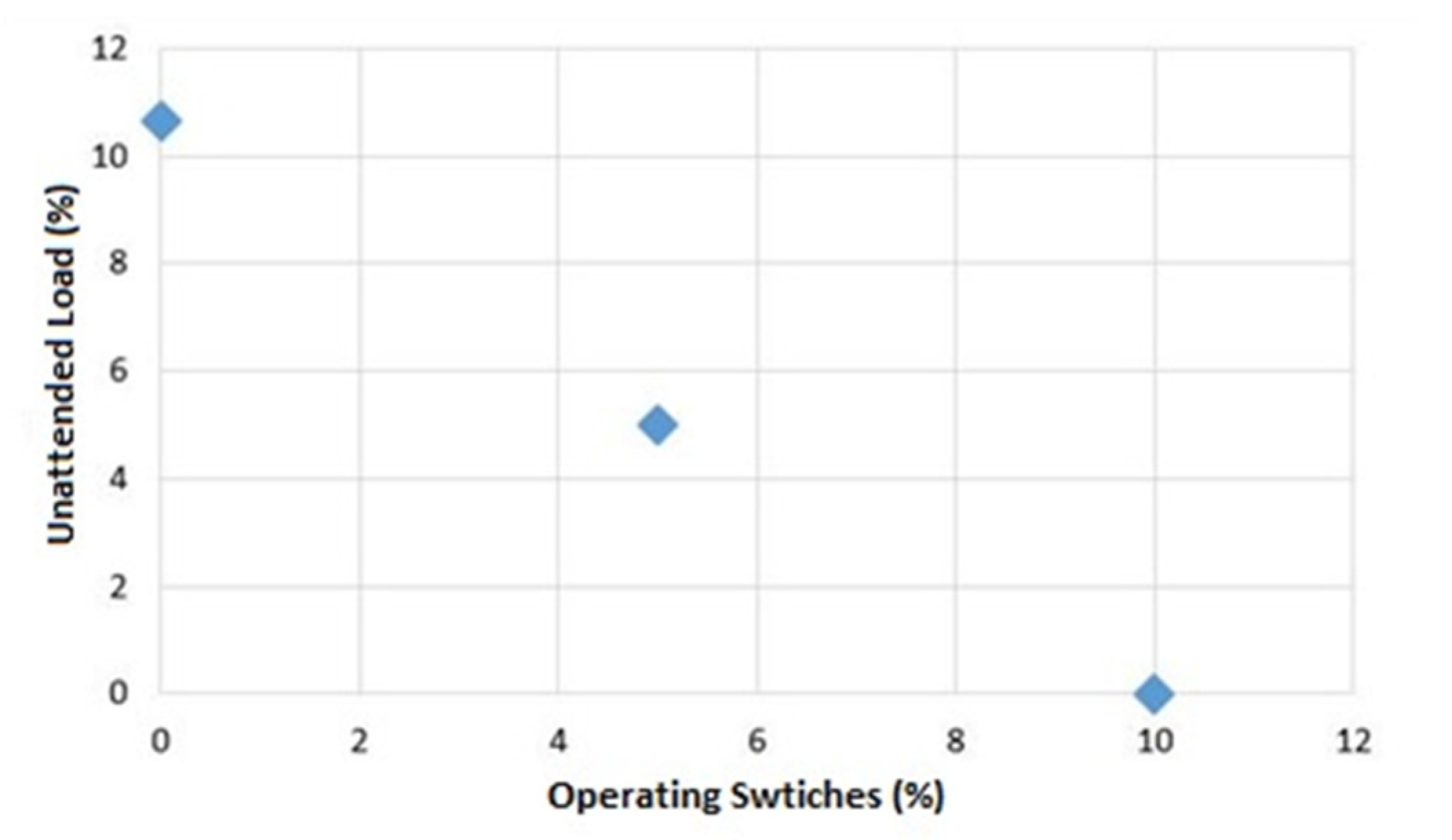
• Maximize the number of loads restored: After calculating the power flow, if all constraints have been respected, all powered buses are added, considering the priorities of each bus.
• Minimize the number of switch operations: A comparison is made between the switch state solution vector with the initial vector to identify the number of changed switches.

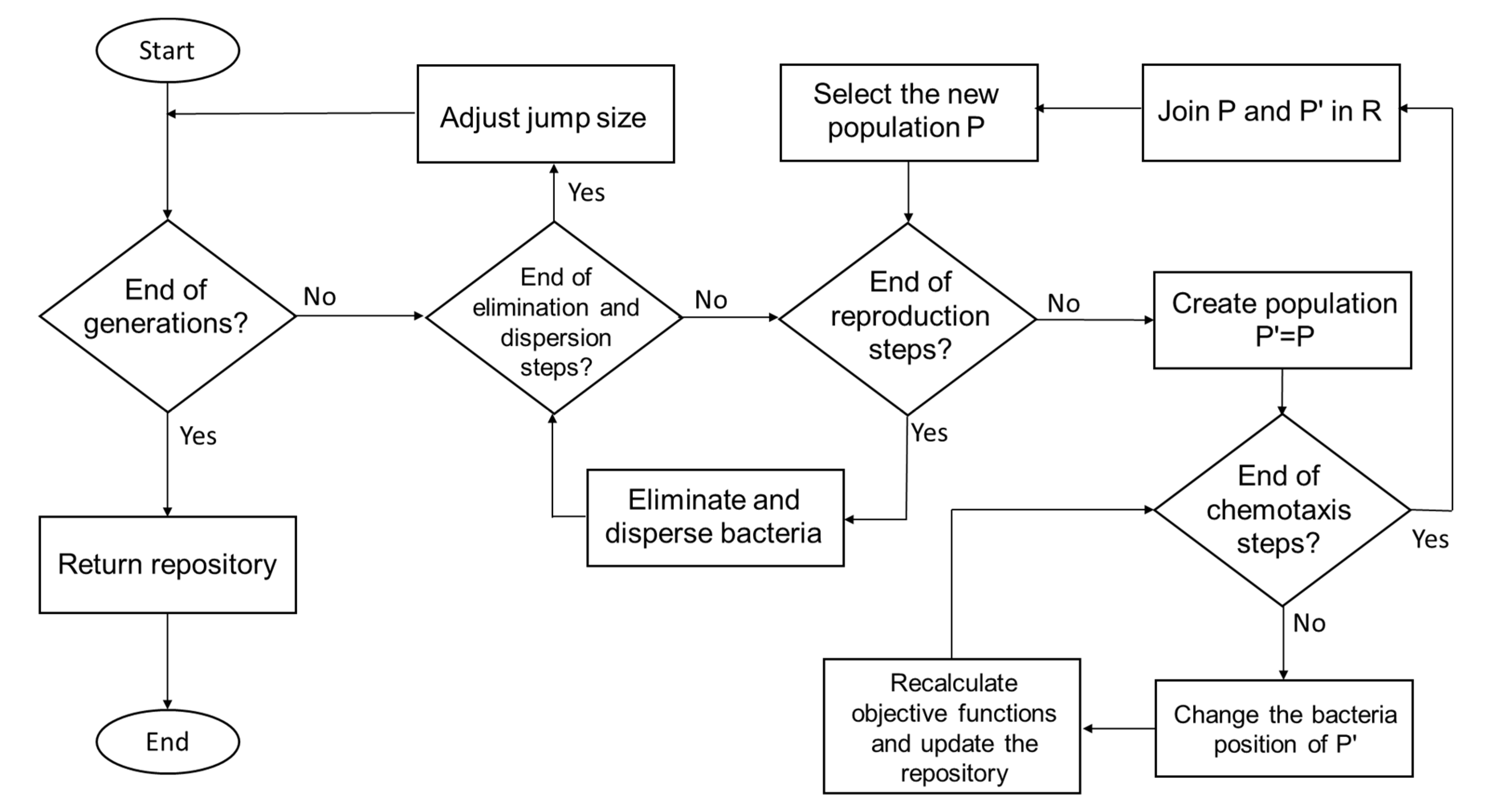
3.5. The Multi-Objective Bacteria Culture Optimization Hybrid Algorithm

The version of MOBFOHA proposed in this paper merges the methodologies proposed in [19,20]. The implementation focuses on changing the stages of selection and reproduction of bacteria so that they do not depend on the health of individuals, making it possible to use the method adapted to a multi-objective more easily. In addition, how bacteria walk through the research space has been changed to a more adaptive version and focused on interaction with the rest of the population, as discussed in more detail in this section. Figure 3 shows the adjustments made in the method concerning the traditional algorithm.

As previously presented, the size of the jump defines the movement of bacteria while scanning the search space. Adjusting this jump size can significantly impact method convergence. A fixed and significant jump size value causes convergence to be achieved faster but can cause the individuals to jump “over” the optimal points, destabilizing the search. Otherwise, a fixed and small value improves the stability of the search but has a slower convergence and can cause the method to end before finding an optimal solution or can cause the solution to come to a great location. Adjusting through generations makes it possible to take advantage of the best benefits during scanning, maintaining stability, improving convergence speed, and avoiding optimal locations.

The proposed MOBFOHA belongs to the class of stochastic algorithms involving random processes. Then each time the algorithm is run, it can give a different answer. Therefore, a suitable adjustment of the initial parameters is essential to obtain reasonable solutions. Another problem is the efficiency of the proposed algorithm. This aspect can be divided into two topics: the time for convergence and the time to provide a restoration solution for a failure in the distribution network. For the first topic, the time for convergence of the algorithm in a large distribution network is not a problem because it does not contain recursive computations. Its order of complexity is O(n). Providing a solution in real-time is not a problem in the second topic. Even though the algorithm is being executed many times, the total time is inferior to the time of the operator’s analysis.

The same problem discussed in implementing the Multiple-Objective Particle Swarm Optimization (MOPSO) version proposed in [32] is considered in this proposed approach. Bacteria should not be attracted to a single point but the Pareto-optimal region. Thus, swarm operations must be adapted so that attraction and repelling interactions respect this characteristic. The version proposed in this paper is simplified and integrated into the chemotaxis stage, as presented in [34]. Each bacterium chooses the direction to move attracted by another dominant bacterium.

Then, given a MOOP with objectives, the algorithm steps and the routines mentioned above are presented in detail below:

• Create N population with S-size and randomly spread individuals through the search space.
• Evaluate each individual for each one of the M objectives.
• Individuals who present solutions not dominated by other individuals are inserted in file P, that is, solutions that are not worse for each of the objectives found and better in at least one goal. These solutions are considered the approximate Pareto border [35].
• The solutions in file A are mapped in the parallel cell coordinate system (PCCS) [32]. That is, each solution receives a label that is an integer between 1 and |A| (size of A) according to the Equation (8), where n is the solution indicator (1, 2, …,|A|), m is the objective indicator, $f_{k,m}$ is the value of solution n, for objective m, $f_m^{max}$ is the highest value found for objective m and $f_m^{min}$ is the lowest value found for objective m. The value is rounded up, and when $f_{k,m}=f_m^{min}$, the value is changed to 1 to avoid division by zero.

  $$L_{k,m}=K \frac{f_{k,m}-f_m^{min}}{f_m^{max}-f_m^{min}}$$

  (8)
• If the file size exceeds the maximum size S, the densities of all solutions must be calculated, and the highest density is eliminated. The density calculation of a solution is done based on the distances between pairs of solutions, as shown in the following equations:

  $$DCP\left(P_i,P_j\right)=\{\begin{array}{c}{{\displaystyle \sum }}_{m=1}^M\left|L_{i,m}-L_{j,m}\right|, if \exists m | L_{i,m}\ne L_{j,m} \\ 0.5, otherwise\end{array} ,$$

  (9)

  $$D\left(P_i\right)={{\displaystyle \sum }}_{j=1}^K\frac{1}{DCP{\left(P_i,P_j\right)}^2} .$$

  (10)
• For each generation, with the values of the labels, the entropy of the population is calculated, which measures the uniformity of the approximation of the Pareto border. Equation (11) shows the entropy calculation for generation t, where K is |A|, M is the number of objectives and $Cel{l}_{k,m}\left(t\right)$ is the number of solutions with the label $L_{k,m}$ in the k-th row and m-th column of the PCCS.

  $$E\left(t\right)=-{\displaystyle \sum }_{k=1}^K{\displaystyle \sum }_{m=1}^M\frac{Cel{l}_{k,m}\left(t\right)}{KM}\log \frac{Cel{l}_{k,m}\left(t\right)}{KM}$$

  (11)
• The adjustment in the jump size of bacteria is made with the differential $\Delta E\left(t\right)=E\left(t\right)-E\left(t-1\right)$ according to the evolutionary state of the population, which can be a state of convergence, state of diversity, and state of stagnation. The threshold for the convergence state is given by ${\delta }_C=\frac{2}{K}log2$ and the threshold for the stagnant state is given by ${\delta }_E=\frac{2}{KS}log2$ where S is the maximum file size.
• Given the thresholds, the adjustment of the jump size C is given by the following equation, where λ and μ are the adjustments and K(t) is the number of solutions in A the generation t.

  $$\begin{gathered} \mathrm{Convergence}:\left|\Delta E\left(t\right)\right|>{\delta }_C\mathrm{or}\left|K\left(t\right)-K\left(t-1\right)\right|>0 \\ \mathrm{Diversity}:{\delta }_C<\left|\Delta E\left(t\right)\right|<{\delta }_E\mathrm{and}K\left(t\right)=K\left(t-1\right)=S \\ \mathrm{Stagnation}:\left|\Delta E\left(t\right)\right|>{\delta }_E\mathrm{and}K\left(t\right)=K\left(t-1\right) \end{gathered}$$

  (12)

  $$C_t\left(i\right)=\{\begin{array}{c}{C}_{t-1}\left(i\right)-\lambda \left(1+\left|\Delta E\left(t\right)\right|\right), if convergence \\ C_{t-1}\left(i\right)+\mu \left|\Delta E\left(t\right)\right|, if diversity\\ C_{t-1}\left(i\right), if stagnation\end{array}$$

  (13)
• For each one of the N_ed steps of elimination and dispersion is made the reproduction process.
• For each of the N_rep steps of reproduction is carried out the process of chemotaxis. A new population is generated P’ copying the values of the population P, and for each step of chemotaxis N_ch, the population P’ is updated recalculating the position of each individual according to the equation (14), where is ${\theta }^i\left(ch,r, ed\right)$ is the position of the i-th bacterium in the ch-th step of chemotaxis, r- th stage of reproduction and ed-th elimination and dispersion step, $\Delta \left(i\right)$ is a random vector that represents the direction in which the bacterium jump and $C_t\left(i\right)$ is the size of the jump.

  $${\theta }^i\left(ch+1,r, ed\right)={\theta }^i\left(ch,r,ed\right)+C_t\left(i\right) \frac{\Delta \left(i\right)}{\sqrt{{\Delta }^T\left(i\right)\Delta \left(i\right)}}$$

  (14)
• All bacteria are evaluated for all purposes, and file P is updated with the previous procedure.
• Once the chemotaxis process is finished, a new population is generated through non-dominance ordering [20]. The N population is merged with the N’ population in a set R. All solutions from the Pareto border are selected. When the number of solutions found is less than S, they are added in the new population N and removed from R. A new Pareto border, that is, the rank 2 border, is selected from R. If the number of members of that border is less than S − |N|, they are also added in N and removed from R, and so on.

If any of the borders cannot be added in N, that is, it is larger than the space available for N to be size S, it is necessary to perform crown distance ordering of the elements of the border [36]. The crowd distance is the average distance between its two neighboring solutions. Sorting elements based on each of the objectives is required. Infinite distance is allocated to solutions with value $f_m^{min}$ and $f_m^{max}$ and the other elements of the border in question have the distance calculated by $F{\left[k\right]}_{distance}=F{\left[k\right]}_{distance}+\left(f_{k+1,m}-f_{k-1,m}\right)/\left(f_m^{max}-f_m^{min}\right)$. Solutions with the highest values are added in N until |N| = S to ensure diversity on the Pareto border. Figure 4 shows how the construction of the new population is made.

13.

Once the reproduction steps are completed, individuals are eliminated and dispersed in the search space with a probability $P_{ed}$.

14.

After the elimination and dispersion steps, a new adjustment in the jump size is made and finished the generations. File P contains the best solutions found.

4. Results and Comparisons in Distribution Networks

The proposed methodology’s effectiveness for restoring an electrical distribution network is evaluated by applying the method in two systems with 70 and 201 buses. Some contingency cases with one and more short-circuit are tested for each system.

4.1. Applying the Proposed Methodology

The method is initially applied to the NO (Normally Open) switches. If any configuration of these switches is sufficient to meet all loads respecting all constraints, the program terminates by returning which or which NO switches should be closed.

After the first run, it is checked if any optimal solutions violate any conductor’s current limit. If this happens, there may be an NC (Normally Closed) switch that eliminates the overhead that occurred. In addition, there may be another NO switch that can be closed to meet the rest of the loads after opening this NC switch. In this way, a second execution of the algorithm is done considering all system switches.

Even if overloads have not occurred during the first run, it is also checked whether any solution reestablishes all the buses outside the isolation area. If this does not happen, the new execution is also performed for the search to continue. It is noteworthy that there may not be a solution that restores 100% of the required load, and the second execution is only performed to ensure that this possible optimal solution was not found in the first.

For each execution, individuals are initialized to optimize the search for the best settings. On the first run, the population is initialized with the value of the initial configuration of the switches after the isolation of the faults. If necessary, the population starts with the best combinations found in the previous run in the second run.

4.2. Parameter Adjustment

The parameters used for the tests were chosen based on studies present in the literature and by observing the convergence of the method. As discussed above, the algorithm runs twice. Each run has an initial configuration of different parameters because they involve other variables.

Table 1. MOBFOHA Parameters.

Parameters	Execution 1	Execution 2
Ned	2	2
ped	0.25	0.25
Nrep	4	4
Nch	60	120
C	50	50
Λ	2	2
Μ	10	10
maxgen	5	10

shows the value chosen for each parameter in the two runs.

4.3. Test System I: 70-Buses Network

The first network used for the tests was presented in [37], and it has been used in many published studies. This network comprises 70 buses, 2 substations, 9 NO switches, and 11 NC switches. The base voltage values are set to 11, and the base power value is 1. The voltage values on the buses must be in the range of 0.8 to 1.05. Current limits are given for each conductor. Figure 5 shows the initial network configuration.

4.3.1. Single Short-Circuit

This section presents two single short-circuits in the feeders 25–26 and 3–4.

Then, for the first experiment, a short-circuit is considered in the feeder between buses 25 and 26. For failure isolation, switches (NC) 8 and 9 are opened and marked, so they are not used in the restoration step and the NO switch 2.

The two Pareto-optimal solutions, present in

Table 2. Pareto-optimal solutions for the 70-buses system with short-circuit in feeder 25–26.

Faulty Feeders	NO Switches	NC Switches	P(%)
25–26	29–64	None	100%
	None	None	94.83%

, are found by performing a brute force analysis of all possible switching combinations. As shown in the table, the first solution meets all the demand by performing maneuvers on 5% of the switches, closing the NO switch 4 to meet buses 28 and 29. The second solution does not operate in the available switches and no longer meets about 5% of the demand power. Loads of buses 28 and 29 are disconnected from the system after isolation. It is noteworthy that the demand of the fault region is subtracted from the total demand during isolation.

The solutions found by the algorithm studied are shown in Figure 6 using the Pareto curve. The method found all optimal solutions in 35 s, using 2400 iterations.

In the second experiment, a short-circuit is considered in the feeder between buses 3 and 4. NC switches 10, 16, and 17 are used in isolation and are therefore marked so that they are not typed in the optimization step.

Again, the optimal solutions in

Table 3. Pareto-optimal solutions for the 70-buses system with short-circuit in feeder 3–4.

Faulty Feeders	NO Switches	NC Switches	P(%)
3–4	67–15	None	100%
	9–50
	67–15	None	95.00%
	None	None	89.34%

are found when performing a brute force analysis. In the first solution, all demand is applied by closing the NO switches 67–15 and 9–50, 10% of the available switches. Only the NO switch 67–15 is closed in the second solution. 5% of the switches and only 5% of the load are not applied. The final solution is the configuration after isolation. About 89.34% of the demand is supplied without any switch changes. Approximately 10.66% of the required load is disconnected from the system. It is important to remember that all optimal settings respect all operating restrictions of the system.

The proposed algorithm also finds all the optimal solutions for this case, taking about 75 s and 2400 iterations. The solutions are shown at the Pareto border in Figure 7.

4.3.2. Double Short-Circuit

This section shows an example where two short-circuit happen at the same time. In this case, the short-circuits occur in the same two feeders of the previous example: between buses 3 and 4 and between buses 25 and 26. The fault isolation process locked the same NC switches: 10, 16, and 17 due to fault in 3–4; and 8 and 9, and NO switch 2, due to 25–26.

After brute force analysis, the solutions presented in

Table 4. Pareto-optimal solutions for the 70-buses system with short-circuit in feeders 3–4 and 25–26.

Faulty Feeders	NO Switches	NC Switches	P(%)
3–4 25–26	9–50 29–64 45–60 9–15	44–45	100%
	22–67 67–15 9–50 29–64	65–66	100%
	22–67 67–15 29–64 9–15	65–66	100%
	9–15 29–64 9–50	44–45	97.56%
	67–15 9–50	None	94.22%
	67–15	None	88.86%
	None	None	89.34%

are found. In this case, performing only the closing of NO switches could not restore all the buses without violating the current limit on some conductors. Therefore, in two solutions, the NC switch 14 must be opened, and in two others, the NC switch 15 is changed.

In Figure 8, the Pareto curve of the solutions found by the proposed algorithm is displayed with the best possible solutions. The solutions are found in 633 s with 12,000 iterations. Figure 9 shows the second of the 5 solutions found. This solution restores all the required load.

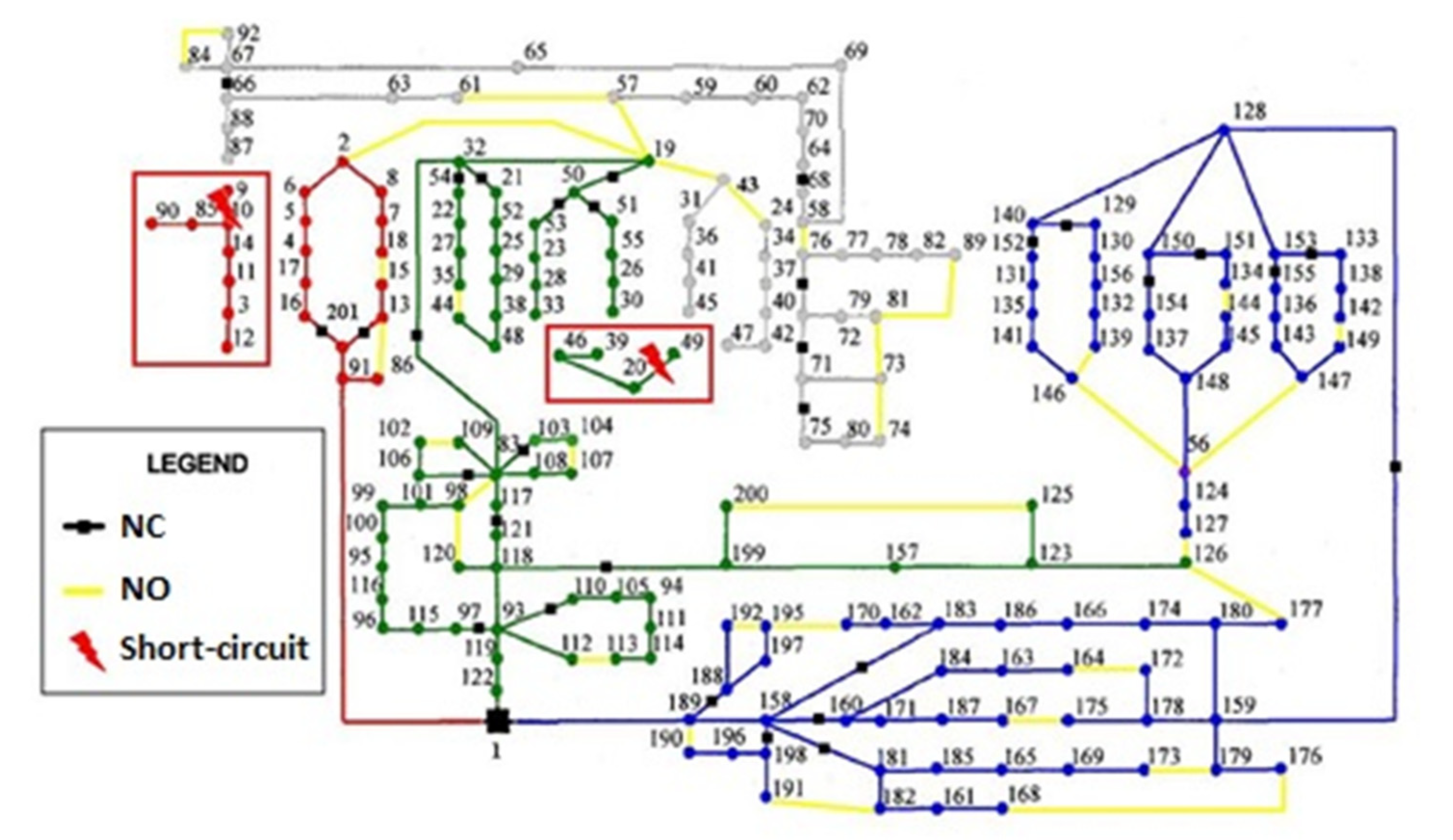
4.4. Test System II: 210-Buses Network

The second system used for the experiments is adapted from [13]. It has 201 buses, one substation with three feeders, 39 NO switches, and 37 NC switches. The base voltage value is 10 kV, and the base power value is 100 kVA. This system does not present the impedance values for the conductors, so the voltage drop calculation is not made, and, consequently, the voltage value for each bus is set at 1 pu. The maximum power of 7983 kW gives the flow limit on the conductors. Thus, the current limit of 79.83 A for each conductor is considered to adapt to the method. Figure 10 shows the initial system configuration.

4.4.1. Single Short-Circuit

This section presents an example considering a short circuit between buss 72 and 79. After isolation, the feeders between buses 76 and 89 are unsupplied.

After the execution of the method, the solutions in

Table 5. Pareto-optimal solutions for the 210-buses system with short-circuit in feeder 72–79.

Faulty Feeders	NO Switches	NC Switches	P(%)
72–79	58–64	None	100%
	None	None	97.77%

are found, shown at the Pareto border in Figure 11. The proposed method used 2400 iterations and took 90 s to deliver all responses.

4.4.2. Double Short-Circuit

A more complex experiment is now performed, where short-circuit happens simultaneously between buses 9 and 10 and between buses 20 and 49. Joint failures disconnect about 30% of network load demand. Figure 12 shows the network configuration after the two faults are isolated.

The first execution of the proposed algorithm failed to restore all the load, although the best solutions found do not violate any operational limit. Therefore, a new execution of the algorithm is made, and, in this case, a solution that meets all the demand can be found.

Table 6. Pareto-optimal solutions for the 210-buses system with short-circuits in feeders 9–10 and 20–49.

Faulty Feeders	NO Switches	NC Switches	P(%)
9–10 20–49	2–19 19–43 19–57 24–43 58–76	117–121	100%
	19–43 19–57 24–43 58–76	83–106	99.02%
	19–43 19–57 58–76	None	95.83%
	19–57 58–76	None	93.14%
	19–57	None	85.48%
	None	None	75.91%

shows all the solutions found, and Pareto’s boundary for these solutions is shown in Figure 13.

The first configuration, which restores all load demand for this case, is shown in Figure 14.

4.4.3. Comparison between Methods

The quality of the found solutions by the proposed approach to the 201-buses system is made by comparing it with the results obtained using the PSO technique proposed in [13] and the GA technique proposed in [38]. Both techniques use only one objective function and consider the other objectives through weighting. However, in different runs, the method finds equally optimal different solutions. Thus, it is possible to compare with a multi-objective method proposed in this work.

First, a set of short-circuits is compared in which the PSO and the GA presented a single solution.

Table 7. Comparison of MOBFOHA, PSO, and GA methods results - Single solution.

Faulty Feeders	MOBFOHA			PSO			GA
	NO	NC	P(%)	NO	NC	P(%)	NO	NC	P(%)
1–91	2–19 20–56	20–48	100%	2–19 20–56	20–48	100%	2–9 19–57 76–58	70–62 67–65	82.62%
	19–57 20–56	20–48	100%	-	-	-	-	-	-
	2–19	12–201	86.75%	-	-	-	-	-	-
	None	None	82.62%	-	-	-	-	-	-
76–77	81–89	None	100%	81–89	None	100%	81–89	None	100%
	None	None	98.16%	-	-	-	-	-	-
93–110	112–113	None	100%	112–113	None	100%	112–113	None	100%
	None	None	95.68	-	-	-	-	-	-
128–140	56–146	None	100%	56–146	None	100%	56–146	None	100%
	None	None	93.62	-	-	-	-	-	-

shows each of these cases and the results found by the two methods in parallel. Observing the solutions on this table, MOBFOHA presents more alternatives to the operators, and new objectives can be applied to find the best solution among the better solutions.

Also, the results in which the PSO and the GA have more than one solution been compared.

Table 8. Comparison of MOBFOHA, PSO, and GA methods results - Multiple solutions.

Faulty Feeders	MOBFOHA			PSO			GA
	NO	NC	P(%)	NO	NC	P(%)	NO	NC	P(%)
1–91	58–76 126–127	117–121	100%	-	-	-	-	-	-
	58–76 126–177	117–121	100%	58–76 126–177	117–121	100%	-	-	-
	19–57 20–56	20–48	100%	19–57 20–56	20–48	100%	-	-	-
	19–57 126–127	117–121	100%	19–57 126–127	117–121	100%	-	-	-
	19–57 126–177	117–121	100%	19–57 126–177	117–121	100%	-	-	-
	2–19 20–56	20–48	100%	-	-	-	-	-	-
	2–19 126–177	117–121	100%	2–19 126–177	117–121	100%	-	-	-
	19–57	117–121	87.68%	-	-	-	-	-	-
	58–76	117–121	87.68%	-	-	-	2–9 19–57	58–68	82.62
	2–19	117–121	87.68%	-	-	-	2–9 19–57 76–58	69–58 19–57	82.62
	None	None	54.51%	-	-	-	-	-	-
1–189	2–19 126–127	117–121	100%	-	-	-	-	-	-
	58–76 126–127	117–121	100%	58–76 126–127	117–121	100%	126–127	-	62.87%
	19–57 126–177	117–121	100%	19–57 126–177	117–121	100%	126–127 126–177	124–127	62.87%
	2–19 126–177	117–121	100%	2–19 126–177	117–121	100%	-	-	-
	58–76 126–177	117–121	100%	58–76 126–177	117–121	100%	58–76 126–177	117–121	100%
	None	None	62.87%	-	-	-	-	-	-
19–32	33–46	None	100%	33–46	None	100%	33–46	None	100%
	2–19	None	100%	2–19	None	100%	2–19	None	100%
	19–43	None	100%	19–43	None	100%	19–43	None	100%
	30–39	None	100%	30–39	None	100%	30–39	None	100%
	None	None	93.91	-	-	-	-	-	-

shows the solutions found. It is possible observing that MOBFOHA finds a more significant number of solutions. Some objective functions considered in the mono-objective method have greater weight than others. Another considerable remark is the solutions found by MOBFOHA are the result of a single random execution of the method. In the case of the PSO and the GA, for each solution found, one execution is performed.

Observing the solutions shown in the previous tables, notice that MOBFOHA finds more solutions. It occurs because some objective functions considered in the mono-objective method have greater weight than others. It is worth noting that the solutions found by MOBFOHA are the result of a single random execution of the method. In the cases of PSO and GA, for each solution found, an execution was performed.

Unlike the PSO and the GA approach, MOBFOHA also considers the solutions that do not restore all the load demanded due to Pareto dominance rules. In this way, the concessionaire can weigh according to the need, choosing the best solution for each specific situation. Previously, weighing the functions makes this type of analysis impossible and should ensure that the best weights are chosen.

5. Conclusions

Through the proposed model, the performance of a version of the bio-inspired technique in bacteria’s foraging strategy can be evaluated. The adaptations made to the multi-objective version proved effective in searching for Pareto-optimal solutions. Through the comparations with the results obtained with the brute force routine in the case of the 70-buses system and with the results obtained by the PSO method for the 201-buses system, it can be noted that the method can deliver all the optimal solutions expected for the cases tested, considering the two proposed objectives.

Multi-objective optimization is very important for the operation of systems. With this approach, solutions that maximize the number of loads served are placed in parallel with others that minimize the number of switchings, even if not serving many loads. Thus, the distribution companies can make the best decision, considering the impact caused for each of the decisions, concerning the difficulty and cost generated to implement the proposed configuration and the possible fine for lack of supply, among other factors not addressed by the solution. In addition, when all other objectives can be considered, such as those suggested as future work, a much more assertive decision can be made, especially in the context of smart grids.

References

1. Del Real, A.J.; Pastor, A.; Durán, J. Generic Framework for the Optimal Implementation of Flexibility Mechanisms in Large-Scale Smart Grids. Energies 2021, 14, 8063. [Google Scholar] [CrossRef]
2. Akil, M.; Dokur, E.; Bayindir, R. The SOC Based Dynamic Charging Coordination of EVs in the PV-Penetrated Distribution Network Using Real-World Data. Energies 2021, 14, 8508. [Google Scholar] [CrossRef]
3. Gu, C.; Zhang, Y.; Wang, J.; Li, Q. Joint planning of electrical storage and gas storage in power-gas distribution network considering high-penetration electric vehicle and gas vehicle. Appl. Energy 2021, 301, 117447. [Google Scholar] [CrossRef]
4. Golshani, A.; Sun, W.; Zhou, Q.; Zheng, Q.P.; Tong, J. Two-Stage Adaptive Restoration Decision Support System for a Self-Healing Power Grid. IEEE Trans. Ind. Inform. 2017, 13, 2802–2812. [Google Scholar] [CrossRef]
5. Siebert, L.C.; Sbicca, A.; Aoki, A.R.; Lambert-Torres, G. A Behavioral Economics Approach to Residential Electricity Consumption. Energies 2017, 10, 768. [Google Scholar] [CrossRef] [Green Version]
6. Esmin, A.A.A.; Lambert-Torres, G.; de Souza, A.C.Z. A hybrid particle swarm optimization applied to loss power minimization. IEEE Trans. Power Syst. 2005, 20, 859–866. [Google Scholar] [CrossRef]
7. Torres, B.S.; Ferreira, L.R.; Aoki, A.R. Distributed Intelligent System for Self-Healing in Smart Grids. IEEE Trans. Power Deliv. 2018, 33, 2394–2403. [Google Scholar] [CrossRef]
8. Poudel, S.; Dubey, A. Critical Load Restoration Using Distributed Energy Resources for Resilient Power Distribution System. IEEE Trans. Power Syst. 2019, 34, 52–63. [Google Scholar] [CrossRef] [Green Version]
9. Li, Y.; Xiao, J.; Chen, C.; Tan, Y.; Cao, Y. Service Restoration Model With Mixed-Integer Second-Order Cone Programming for Distribution Network With Distributed Generations. IEEE Trans. Smart Grid 2019, 10, 4138–4150. [Google Scholar] [CrossRef]
10. Gush, T.; Bukhari, S.B.A.; Haider, R.; Admasie, S.; Oh, Y.U.; Cho, G.Y.; Kim, C.H. Fault detection and location in a microgrid using mathematical morphology and recursive least square methods. Int. J. Electr. Power Energy Syst. 2018, 102, 324–331. [Google Scholar] [CrossRef]
11. Eberhart, R.; Kennedy, J. A new optimizer using particle swarm theory. In Proceedings of the Sixth International Symposium on Micro Machine and Human Science, Nagoya, Japan, 4–6 October 1995; pp. 39–43. [Google Scholar] [CrossRef]
12. Holland, J.H. Genetic Algorithms and the Optimal Allocation of Trials. SIAM J. Comput. 1973, 2, 88–105. [Google Scholar] [CrossRef]
13. Lambert-Torres, G.; Martins, H.G.; Coutinho, M.P.; Salomon, C.P.; Vieira, F.C. Particle Swarm Optimization applied to system restoration. In Proceedings of the 2009 IEEE Bucharest PowerTech, Bucharest, Romania, 28 June–2 July 2009; pp. 1–6. [Google Scholar] [CrossRef]
14. Lin, W.-C.; Huang, W.-T.; Yao, K.-C.; Chen, H.-T.; Ma, C.-C. Fault Location and Restoration of Microgrids via Particle Swarm Optimization. Appl. Sci. 2021, 11, 7036. [Google Scholar] [CrossRef]
15. Zou, K.; Mohy-ud-din, G.; Agalgaonkar, A.P.; Muttaqi, K.M.; Perera, S. Distribution System Restoration with Renewable Resources for Reliability Improvement Under System Uncertainties. IEEE Trans. Ind. Electron. 2020, 67, 8438–8449. [Google Scholar] [CrossRef]
16. Mendoza, J.; Lopez, R.; Morales, D.; Lopez, E.; Dessante, P.; Moraga, R. Minimal loss reconfiguration using genetic algorithms with restricted population and addressed operators: Real application. IEEE Trans. Power Deliv. 2006, 21, 948–954. [Google Scholar] [CrossRef]
17. Tomoiagă, B.; Chindriş, M.; Sumper, A.; Sudria-Andreu, A.; Villafafila-Robles, R. Pareto Optimal Reconfiguration of Power Distribution Systems Using a Genetic Algorithm Based on NSGA-II. Energies 2013, 6, 1439–1455. [Google Scholar] [CrossRef] [Green Version]
18. Čađenović, R.; Jakus, D.; Sarajčev, P.; Vasilj, J. Optimal Distribution Network Reconfiguration through Integration of Cycle-Break and Genetic Algorithms. Energies 2018, 11, 1278. [Google Scholar] [CrossRef] [Green Version]
19. Niu, B.; Wang, H.; Wang, J.; Tan, L. Multi-objective bacterial foraging optimization. Neurocomputing 2013, 116, 336–345. [Google Scholar] [CrossRef]
20. Kaur, M.; Kadam, S. A novel multi-objective bacteria foraging optimization algorithm (MOBFOA) for multi-objective scheduling. Appl. Soft Comput. 2018, 66, 183–195. [Google Scholar] [CrossRef]
21. Dorigo, M.; Maniezzo, V.; Colorni, A. Ant system: Optimization by a colony of cooperating agents. IEEE Trans. Syst. Man Cybern. Part B 1996, 26, 29–41. [Google Scholar] [CrossRef] [Green Version]
22. Selva Rani, B.; Aswani Kumar, C. A Comprehensive Review on Bacteria Foraging Optimization Technique. In Multi-Objective Swarm Intelligence. Studies in Computational Intelligence; Dehuri, S., Jagadev, A., Panda, M., Eds.; Springer: Berlin/Heidelberg, Germany, 2015; Volume 592. [Google Scholar] [CrossRef]
23. Panda, A.; Pani, S. A Symbiotic Organisms Search algorithm with adaptive penalty function to solve multi-objective constrained optimization problems. Appl. Soft Comput. 2016, 46, 344–360. [Google Scholar] [CrossRef]
24. Ustun, D.; Çarbas, S.; Toktas, A. A symbiotic organisms search algorithm-based design optimization of constrained multi-objective engineering design problems. Eng. Comput. 2020, 38, 632–658. [Google Scholar] [CrossRef]
25. Passino, K.M. Biomimicry of bacterial foraging for distributed optimization and control. IEEE Control. Syst. Mag. 2002, 22, 52–67. [Google Scholar] [CrossRef]
26. Berg, H.; Brown, D. Chemotaxis in Escherichia coli analysed by Three-dimensional Tracking. Nature 1972, 239, 500–504. [Google Scholar] [CrossRef] [PubMed]
27. Zhang, Z.; Long, K.; Wang, J.; Dressler, F. On Swarm Intelligence Inspired Self-Organized Networking: Its Bionic Mechanisms, Designing Principles and Optimization Approaches. IEEE Commun. Surv. Tutor. 2014, 16, 513–537. [Google Scholar] [CrossRef]
28. Li, Z.; Tian, M.; Zhao, Y.; Zhang, Z.; Ying, Y. Development of an Integrated Performance Design Platform for Residential Buildings Based on Climate Adaptability. Energies 2021, 14, 8223. [Google Scholar] [CrossRef]
29. Nasrullah, A.I.H.; Puji Santosa, S.; Widagdo, D.; Arifurrahman, F. Structural Lattice Topology and Material Optimization for Battery Protection in Electric Vehicles Subjected to Ground Impact Using Artificial Neural Networks and Genetic Algorithms. Materials 2021, 14, 7618. [Google Scholar] [CrossRef]
30. Qi, J.; Wu, D. Green Energy Management of the Energy Internet Based on Service Composition Quality. IEEE Access 2018, 6, 15723–15732. [Google Scholar] [CrossRef]
31. Yi, J.; Huang, D.; Fu, S.; He, H.; Li, T. Multi-Objective Bacterial Foraging Optimization Algorithm Based on Parallel Cell Entropy for Aluminum Electrolysis Production Process. IEEE Trans. Ind. Electron. 2016, 63, 2488–2500. [Google Scholar] [CrossRef]
32. Hu, W.; Yen, G.G. Adaptive Multiobjective Particle Swarm Optimization Based on Parallel Cell Coordinate System. IEEE Trans. Evol. Comput. 2015, 19, 1–18. [Google Scholar] [CrossRef]
33. Mansour, M.R.; Santos, A.C.; London, J.B.; Delbem, A.C.B.; Bretas, N.G. Energy restoration in distribution systems using multi-objective evolutionary algorithm and an efficient data structure. In Proceedings of the 2009 IEEE Bucharest PowerTech, Bucharest, Romania, 28 June–2 July 2009; pp. 1–7. [Google Scholar] [CrossRef]
34. Pandi, V.R.; Panigrahi, B.K.; Hong, W.C.; Sharma, R. A multi-objective bacterial foraging algorithm to solve the environmental economic dispatch problem. Energy Sources Part B Econ. Plan. Policy 2014, 9, 236–247. [Google Scholar] [CrossRef]
35. Zaenudin, E.; Kistijantoro, A.I. pSPEA2: Optimization fitness and distance calculations for improving Strength Pareto Evolutionary Algorithm 2 (SPEA2). In Proceedings of the 2016 International Conference on Information Technology Systems and Innovation (ICITSI), Bandung, Indonesia, 24–27 October 2016; pp. 1–5. [Google Scholar] [CrossRef]
36. Deb, K.; Pratap, A.; Agarwal, S.; Meyarivan, T. A fast and elitist multiobjective genetic algorithm: NSGA-II. IEEE Trans. Evol. Comput. 2002, 6, 182–197. [Google Scholar] [CrossRef] [Green Version]
37. Das, D. A fuzzy multiobjective approach for network reconfiguration of distribution systems. IEEE Trans. Power Deliv. 2006, 21, 202–209. [Google Scholar] [CrossRef]
38. Salomon, C.P.; Coutinho, M.P.; de Moraes, C.H.V.; Borges da Silva, L.E.; Lambert-Torres, G.; Aoki, A.R. Applications of Genetic Algorithm in Power System Control Centers. In Genetic Algorithms in Applications; Popa, R., Ed.; InTech: London, UK, 2012; pp. 201–222. [Google Scholar] [CrossRef] [Green Version]
Figure 1. Flowchart of BFOA steps.
Energies 15 01445 g001
Figure 2. Flowchart of the proposed method.
Energies 15 01445 g002
Figure 3. Flowchart of the MOBFOHA.
Energies 15 01445 g003
Figure 4. Construction of the new population.
Energies 15 01445 g004
Figure 5. Test system I: 70-buses network [37].
Energies 15 01445 g005
Figure 6. Pareto border for 70 buses system with short-circuit in feeder 25–26.
Energies 15 01445 g006
Figure 7. Pareto border for 70 buses system with short-circuit in feeder 3–4.
Energies 15 01445 g007
Figure 8. Pareto border for 70 buses system with short-circuit in feeders 3–4 and 25–26.
Energies 15 01445 g008
Figure 9. Optimal configuration after the restoration of the system of 70 bus with faults in 3–4 and 25–26.
Energies 15 01445 g009
Figure 10. Test system II: 210-buses network [13].
Energies 15 01445 g010
Figure 11. Pareto border for 210 buses system with short-circuit in feeder 72–79.
Energies 15 01445 g011
Figure 12. Test system II: 210-buses network after the isolation process with short-circuits in the feeders 9–10 and 20–49.
Energies 15 01445 g012
Figure 13. Pareto border for 210 buses system with short-circuits in feeders 9–10 and 20–49.
Energies 15 01445 g013
Figure 14. Test system II: 210-buses network after the restoration process with short-circuits in the feeders 9–10 and 20–49.
Energies 15 01445 g014