Article

Linear Quadratic Regulator and Fuzzy Control for Grid-Connected Photovoltaic Systems

1
Department of Robotics and Mechatronics, School of Engineering and Digital Sciences, Nazarbayev University, Nur-Sultan 010000, Kazakhstan
2
Graduate School of Engineering, Toyota Technological Institute, Nagoya 468-8511, Japan
*
Authors to whom correspondence should be addressed.
Energies 2022, 15(4), 1286; https://doi.org/10.3390/en15041286
Submission received: 2 December 2021 / Revised: 30 January 2022 / Accepted: 1 February 2022 / Published: 10 February 2022
(This article belongs to the Special Issue Energy Transfer in Alternative Vehicles)

Abstract

:
This work presents a control scheme to control a grid-connected single-phase photovoltaic (PV) system. The considered system has four 250 W solar panels, a non-inverting buck-boost DC-DC converter, and a DC-AC inverter with an inductor-capacitor-inductor (LCL) filter. The control system aims to track and operate at the maximum power point (MPP) of the PV panels, regulate the voltage of the DC link, and supply the grid with a unity power factor. To achieve these goals, the proposed control system consists of three parts: an MPP tracking controller module with a fuzzy-based modified incremental conductance (INC) algorithm, a DC-link voltage regulator with a hybrid fuzzy proportional-integral (PI) controller, and a current controller module using a linear quadratic regulator (LQR) for grid-connected power. Based on fuzzy control and an LQR, this work introduces a full control solution for grid-connected single-phase PV systems. The key novelty of this research is to analyze and prove that the newly proposed method is more successful in numerous aspects by comparing and evaluating previous and present control methods. The designed control system settles quickly, which is critical for output stability. In addition, as compared to the backstepping approach used in our past study, the LQR technique is more resistant to sudden changes and disturbances. Furthermore, the backstepping method produces a larger overshoot, which has a detrimental impact on efficiency. Simulation findings under various weather conditions were compared to theoretical ones to indicate that the system can deal with variations in weather parameters.

1. Introduction

Renewable energy is emerging as one of the main sources of energy for the future. The key reason for this is the depletion and pollution of fossil fuels. Renewable energy sources are available, clean, eco-friendly, and cost-effective. There are various types of renewable energy sources, of which solar and wind energy systems have become more and more popular in many countries. According to [1,2], harmonic resonances, which often occur in grid-connected wind power farms, cause negative effects on the power quality of the grid.
Nowadays, solar energy is widely used around the world and demonstrates impressive results. To effectively obtain electricity from solar energy, photovoltaic (PV) systems should be installed. The system efficiency is strongly affected by two major factors, as follow [3,4]:
(a)
Weather factors such as the temperature and solar radiation;
(b)
Hardware factors such as power electronic devices and system loads.
While the prior factor is uncontrollable, the second one depends on the designer, system operator and electric grid. To improve the efficiency of the power electronic parts, appropriate converter topologies together with efficient control schemes are required. From [5,6,7,8], there are two modes of operation for the PV systems, which are:
  • Stand-alone mode;
  • Grid-connected mode.
Between these two modes of operation, the grid-connected mode is preferable, as it can avoid the issues of storage systems in the stand-alone mode. For grid-connected systems, the following two problems need to be solved simultaneously [7,8,9]:
  • Management of several combined systems;
  • Regulation of each power stage or system.
Solving the second problem often requires the following tasks:
  • tracking the maximum power point (MPP);
  • minimizing the harmonics, which usually cause negative effects on the power grid and devices;
  • maintaining the DC-link voltage within a desired range;
  • keeping the unity power factor (PF) at the output of the filter [10].
One of the most important parts of this research is the MPP tracking part, which is mainly used to find and keep the output power of a PV panel at its maximum value [11,12,13]. The MPP tracking (MPPT) technique can be divided into two main categories: the perturb and observe (PO) technique and the incremental conductance (INC) algorithm. The negative side of the PO algorithm is its high computational complexity, but it leads to high efficiency. It measures voltage and current values to periodically estimate the power of the solar panel and compares it with the previous power. If the power of the PV module has increased (dP/dV > 0), the system will start adjustments in that direction; otherwise, it will adjust in the opposite way. These operations continue until system finds the MPP. In fact, the technique depends on perturbations of the voltage, so if the perturbations are high, the speed of the technique is fast. The advantages of this method are simplicity without interest in the previous PV characteristics; however, the main drawback is that oscillations happening near the MPP, which may lead to power losses in varying weather conditions [10]. The INC type is more advantageous in terms of accuracy in finding and tracking the MPP compared to the second type; therefore, in this paper, the INC algorithm is improved by fuzzy control and then implemented in the grid-connected PV system.
Considering current controller strategies, generally, they can be divided into two main categories: on/off controllers and pulse width modulation (PWM)-based control techniques [14]. The first group has two subdivisions, which are hysteresis control and predictive control. Hysteresis control has high dynamics and fast response; however, its major drawbacks are variations of the switching frequency and high complexity of the system. Predictive control has positive sides such as less computation time, better regulation, and a decrease in offset error. On the other hand, it requires identifying a proper model for the system and the installation cost of the system is high. The second group can be divided into linear and non-linear control [14]. Proportional-integral (PI) controller and its different update versions such as multiple generalized integral (MGI) [15] and Manta Ray Foraging Optimization [16] control are the well-known classical control techniques, along with their improved versions, which can be easily designed to control the current. However, the key disadvantage of this controller is its poor compensation of lower-order harmonics and presence of steady-state errors [17]. The proportional-resonant (PR) controlled can compensate for the harmonics. Moreover, this type of controller has high dynamics, is less complex, and can reach a high gain at the resonance frequency. However, this controller has problems reaching the power factor control, which means that the system is not able to control the losses in the system [18].
Generally, the power factor is a ratio between working power and apparent power. Thus, if there is no control/maintenance of a high-power factor, the system efficiency is consequently low. On the other hand, predictive deadbeat control has a high level of harmonic compensation and rapid fast-tracking performance. The disadvantage of this controller is that it requires a lot of computation effort [19]. Harmonic compensation and steady-state error can also be done by repetitive controllers; their slow tracking response is their main drawback [20]. In various dynamic conditions, the effectiveness of the third order complex filter (TOCF) control algorithm may be demonstrated. This controller serves as a distribution static compensator, enhances grid power quality by reducing harmonics, and balances grid currents while maintaining a unity power factor. However, the controller’s biggest disadvantage is its enormous computational load [21]. Another method which possibly could be proposed for mitigation of the issue is the model predictive control (MPC) method [22] and its improved versions [23,24]. However, these methods present oscillations when the load varies. In addition, the THD of MPC is higher compared to other methods, which makes the technique unsuitable for implementation in this case. There exist different kinds of adaptive filtering techniques, such as leaky least mean mixed norm (LLMMN), least mean mixed norm (LMMN), and least mean square (LMS). However, all of the above-mentioned adaptive approaches have the drawback of being unable to maintain acceptable performance in the presence of DC-offset [25]. The combined affine projection sign algorithm (CAPSA) has high stability and tracking performance, but output has the same problem as the previous mentioned method, which is the high THD [26]. Artificial neural networks (ANN) also can be implemented as controllers in this system, but the main disadvantage are their low output power compared to fuzzy logic [27]. Fuzzy logic controllers (FLC) [14] are one of the popular intelligent control techniques. They are extensively used in renewable energy systems due to their efficiency and ease of use. They are also robust and applicable to a wide range of the dynamics systems, from linear to nonlinear systems. Moreover, this type of controller can perform complex estimations, which are not possible with conventional methods [11]. The linear quadratic regulator (LQR) is an effective control method that is applicable for both linear and nonlinear systems. In this method, the control gain is designed to minimize a quadratic cost function by selection of appropriate weighting matrices. In our study case, the cost function is the quadratic function of the tracking error between the current and its reference and the control efforts. This technique was chosen to be implemented due to its properties such as stability, robustness, and ease in application. Moreover, the computational complexity of the LQR controller is not high, which means that it is fairly simple to implement.
This paper proposes a complete control solution for grid-connected single-phase PV systems based on fuzzy control and an LQR. Our past related research on this topic was conducted with a different type of controller, namely the backstepping approach. The present study is a significant extension and improvement of our former research in terms of enhancing the quality of the control method. The proposed technique is the LQR in appropriate combination with fuzzy control and improved INC algorithms for grid-connected photovoltaic systems; furthermore, detailed explanations on developing the fuzzy association rules of the designed fuzzy logic controllers are newly presented in this study. The main originality of this paper is to show and prove by comparison of our former and present control methods that the newly suggested method is more effective in various aspects. Specific details of the PV system and controllers can be found in our past work in [28], which was used as the basis for this paper. The major advantage of the LQR method is its ability to react in a rapid manner to changes of the system, namely, changes in the module temperature or solar irradiation. In other words, the system can reach its settling time faster, which is important to stabilize the behavior of output. Moreover, it can be said that the LQR technique is robust when faced with different disturbances and changes compared to the backstepping technique and its improved fault tolerant version [29]. In addition, the backstepping method has a higher overshoot, which significantly impacts efficiency in a negative way. As was mentioned above, the speed of the LQR is faster, which makes this kind of controller preferable. These are the key contributions of this study compared to our past research in [28]. Simulation results under different weather conditions show that the proposed control system can cope with changes in weather parameters effectively, and were compared with theoretical ones. Moreover, it was shown that variations in weather parameters do not significantly affect the performance of the proposed control system.
The remains of the paper are organized as follows. Section 2 shows the modeling of the grid-connected PV system, which includes the system description, PV panel model, and modeling of power converters. The control system design is depicted in Section 3, which consists of the MPPT control module, DC-link voltage regulator module, and current controller module. In addition, Section 4 provides simulation results in MATLAB, in which the first test case is with a fixed module temperature, and the second test case is with an unchanged solar irradiation. A detailed comparison and assessment of efficacy between the LQR control method in this study and the backstepping approach in our past work [28] is presented in Section 5; brief comparisons between this research and other related works are also shown in this section. The conclusions are described in the last section.

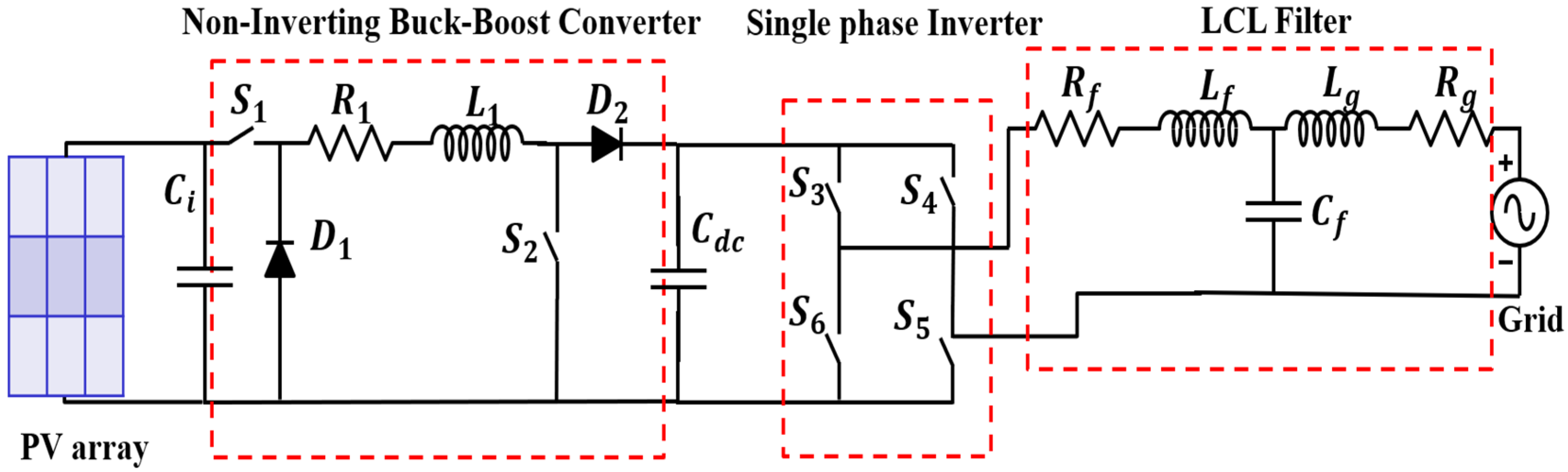
2. PV Grid-Connected System Modeling

2.1. System Description
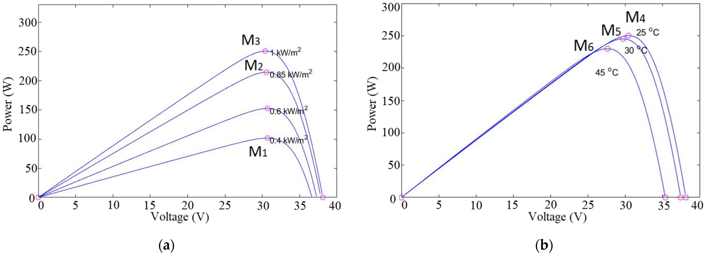
This paper considers a grid-connected PV system consisting of two stages of power conversion. The nominal power of the system is 1 kW. Figure 1 shows the circuitry of the system; the power generated from the PV array is directed to the non-inverting buck-boost DC-DC converter. After that, to supply the grid, the obtained result is converted to AC via the single-phase DC-AC inverter. To remove unwanted noises and disturbances injected to the grid, the LCL output filter was used [30,31].

2.2. PV Panel Model

The PV panels used in this paper have characteristics as presented in [28]. The provided data is applicable when the module temperature is 25 °C and the solar radiation is 1000 W/m2. In total, the PV array consists of four panels, where the nominal power of each panel is 250 W. Figure 2 shows the impacts of module temperature and solar radiation on the power and voltage of the PV panel, respectively. Table 1 represents MPPs of the PV panel and array in terms of power and voltage.

2.3. Modeling of Converters

Figure 1 illustrates all components of the system including the single-phase inverter and the non-inverting buck-boost converter [7]. The input control signals of the non-inverting buck-boost converter and the single-phase inverter are αp and βp, respectively.
α p = { 0 ;   S 1   and   S 2   are   OFF 1 ;   S 1   and   S 2   are   ON β p = { 1 ;   S 3   and   S 5   are   ON ,   S 4   and   S 6   are   OFF 0 ;   S 3 ,   S 4 ,   S 5   and   S 6   are   OFF       1 ;   S 3   and   S 5   are   OFF ,   S 4   and   S 6   are   ON
The modeling technique, specifically averaging, and Kirchhoff’s laws were used to estimate a mathematical model for the two converters. Equation (1) and Table 2 demonstrate details of the previously mentioned procedure
{ x ˙ 1 = 1 C i I - P α 1 C i x 2 x ˙ 2 = α 1 L 1 x 1 R 1 L 1 x 2 + ( α 1 ) 1 L 1 x 3 x ˙ 3 = ( 1 α ) 1 C D C x 2 β 1 C D C x 4 x ˙ 4 = β 1 L f x 3 R f L f x 4 1 L f x 5 x ˙ 5 = 1 C f x 4 1 C f x 6 x ˙ 6 = 1 L g x 5 R g L g x 6 1 L g V g

3. Control System Design

The design of the control system considered in this study is shown in Figure 3 and includes three main parts: the MPPT controller, the DC link voltage regulator, and the current controller. In this paper, detailed explanations on developing the fuzzy rules of the two designed fuzzy logic controllers are presented, which are useful as references for designing other fuzzy controllers.

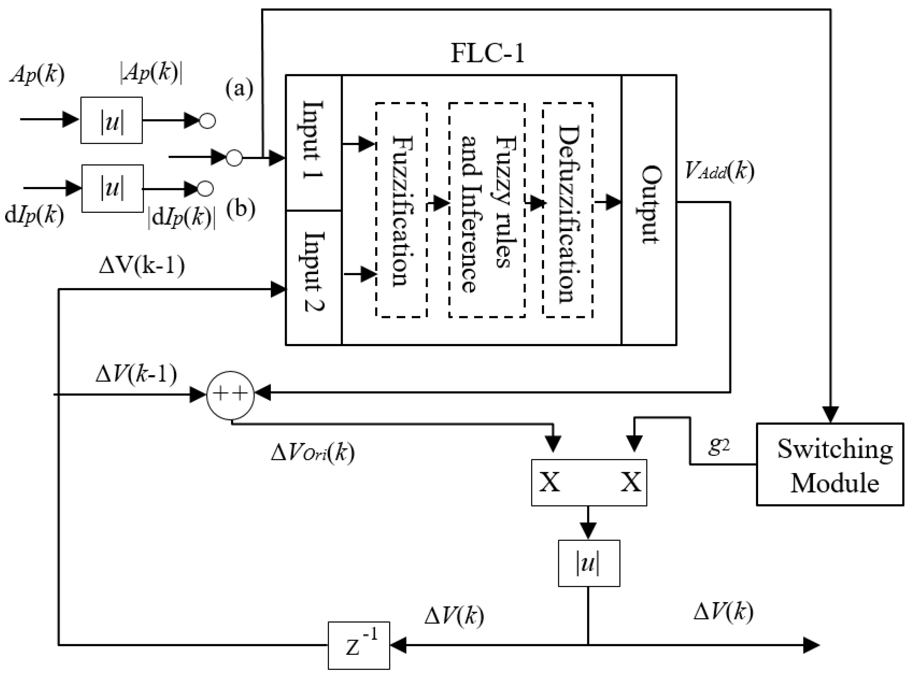
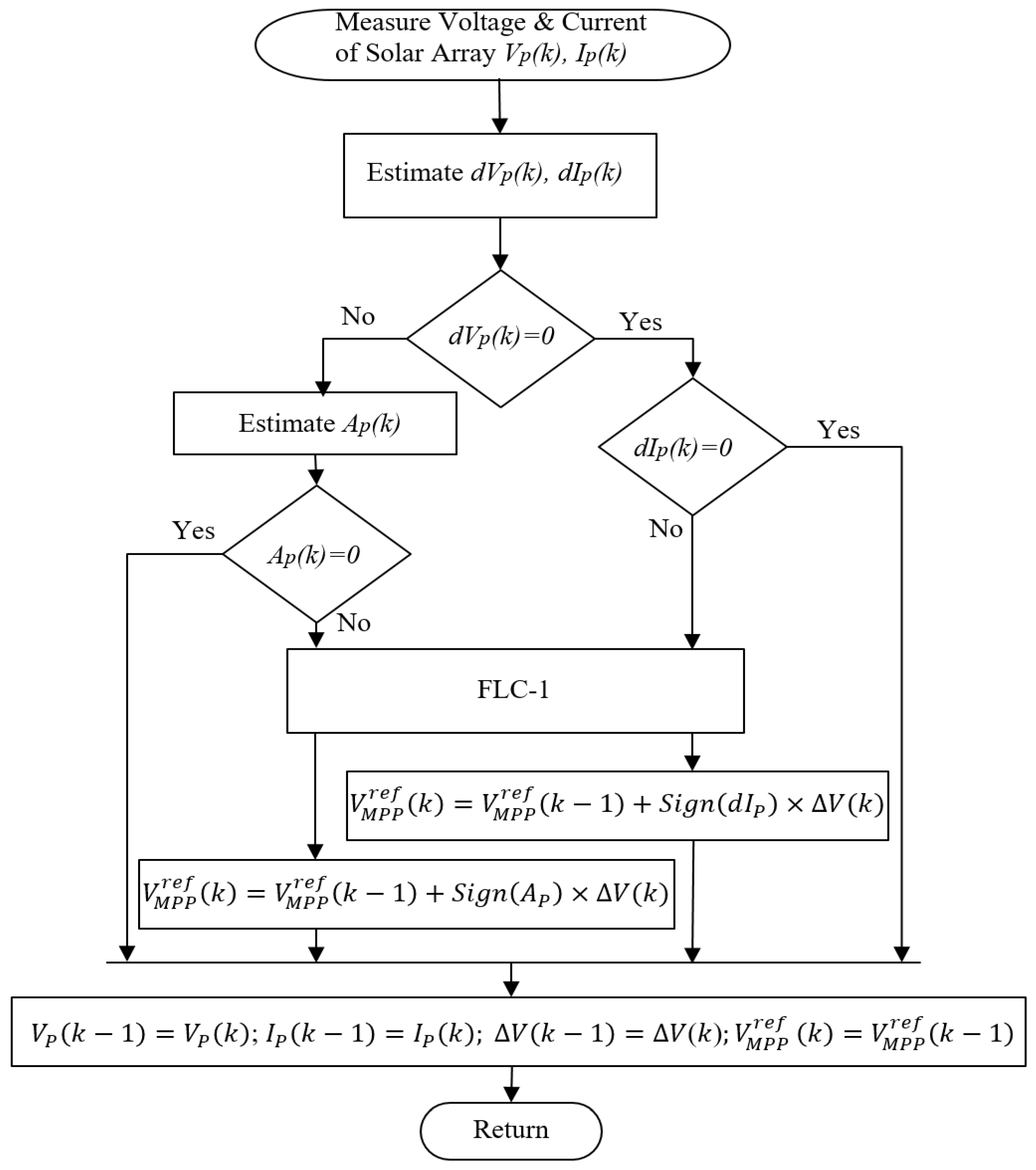
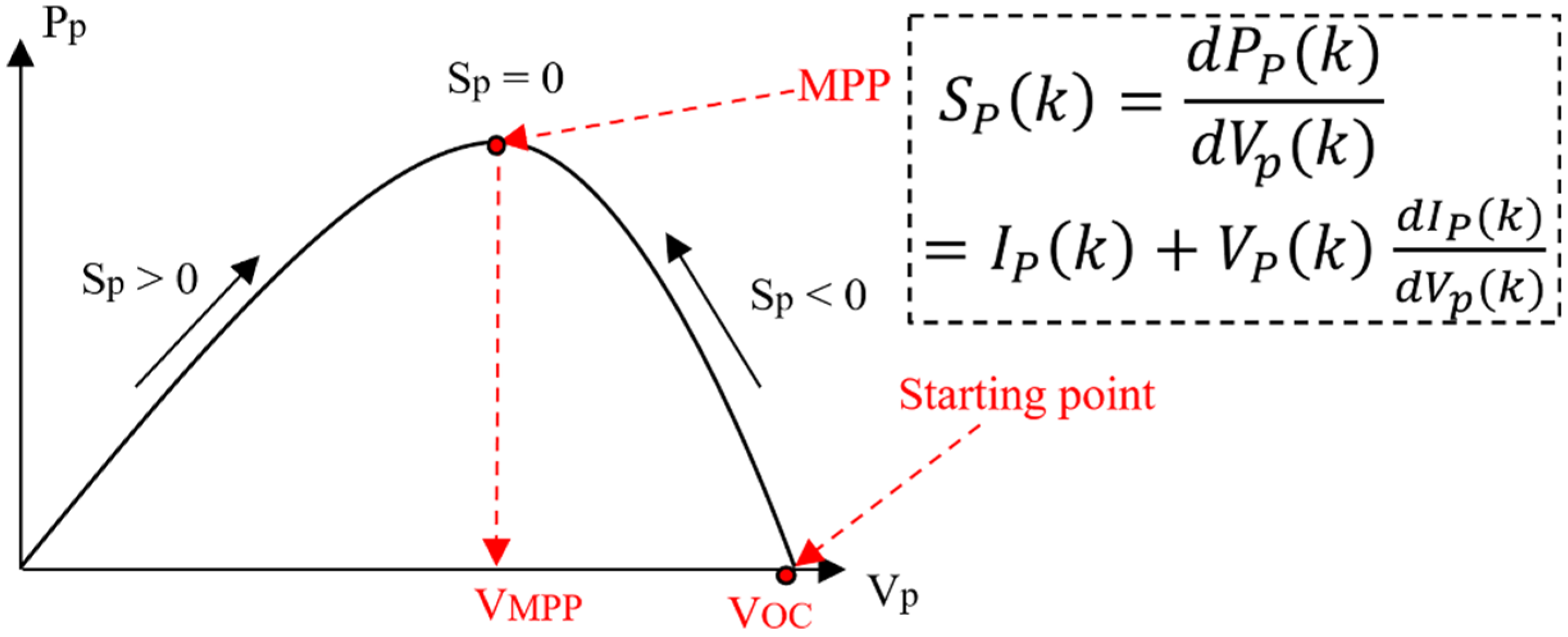
3.1. The MPPT Controller Module

The PV array produces its optimal power despite varying weather with the help of the designed MPPT controller. According to Figure 4, this controller has two parts: the first fuzzy logic controller (FLC-1) and the proportional-integral (PI-1) controller.

3.1.1. FLC-1

The main idea of this sub-controller is to improve the conventional INC-MPPT algorithm in terms of response time and efficiency by combining it with a fuzzy logic controller (FLC-1). According to Figure 5, the FLC-1 has two inputs and one output. The first input can be one of the following two kinds:
  • |Ap(k)|—the absolute value of a modified slope of the power–voltage (P-V) curve as expressed in (2). This equation also includes a pre-scaling module Gp(k), as shown in (3);
  • |dIp(k)|—the change in the current of PV panels in absolute value.
A P ( k ) = G P ( k ) [ S P ( k ) ] = G P ( k ) [ I p ( k ) + V p ( k ) d I P ( k ) d V P ( k ) ]
G P ( k ) = 1 1 + g 1 [ P P ( k ) P P , t o t a l m a x ]
where P P , t o t a l m a x   = 1000 W is the maximum power of PV panels and g1 is a positive coefficient. The second input is the INC algorithm’s prior step-size ΔV(k−1). Figure 6 shows the detailed flowchart of the proposed method. In addition, the aforementioned scaling module Gp(k) is used to suitably increase the sensitivity of slope Sp(k) as given in Figure 7.
lim P p ( k ) 0 G P ( k ) = 1 ,   lim P p ( k ) P P , t o t a l max G P ( k ) = 1 1 + g 1  
P P ( k ) = V P ( k ) × I P ( k )
d I P ( k ) = I P ( k ) I P ( k 1 )
d V P ( k ) = V P ( k ) V P ( k 1 )
To avoid significant changes in the step-size and instability of the PV output power, a switching module is implemented as described in Figure 5. According to the first input, namely, |Ap(k)| or |dIp(k)|, the system will use the appropriate output coefficient g2 as shown in Table 3.
As is known from previous parts of this paper, the inputs are in the range of [0,1]. It should be noted that all the inputs have the same number of linguistic variables, specifically five linguistic variables: VS—Very Small, SM—Small, ME—Medium, LA—Large, VL—Very Large. The output has nine linguistic variables in a range of [−1;1]; in detail, NL—Negative Large, NM—Negative Medium, NS—Negative Small, NZ—Negative Zero, ZE—Zero, PZ—Positive Zero, PS—Positive Small, PM—Positive Medium, PL—Positive Large. As a result, there are 49 fuzzy rules associated in the FLC-1.
All the association rules of the FLC-1 are shown in Table 4, while the membership functions of the inputs and output can be referred to in [28]. To explain the fuzzy rules in Table 4, we can analyze several sample cases as follows. In the first case, when the two inputs ΔV(k−1) and |dIp(k)| are VS, that means that the PV system is close to the MPP and the step voltage is also very small; thus, the output of the FLC-1 as the additional voltage Vadd(k) should be ZE to avoid fluctuations in the PV voltage at the steady state. Whereas, in another case when ΔV(k−1) is LA and |dIp(k)| is ME, the additional voltage Vadd(k) will be NZ because the tendency of the PV system is automatically approaching the MPP. On the other hand, when ΔV(k−1) is vs. and |dIp(k)| is VL, it means that the PV system is far from the MPP; therefore, the output ΔV(k−1) should be PL to force the PV system to quickly move to the MPP. Furthermore, when |dIp(k)| is VL and ΔV(k−1) is VL, the output ΔV(k−1) can be chosen as either PZ or ZE for the PV system to automatically move to the MPP; in this study, we want to increase the speed for searching the MPP, so the output ΔV(k−1) is set as PZ in this case. In general, the other fuzzy rules in Table 4 can be suitably interpreted with the same deductive method.

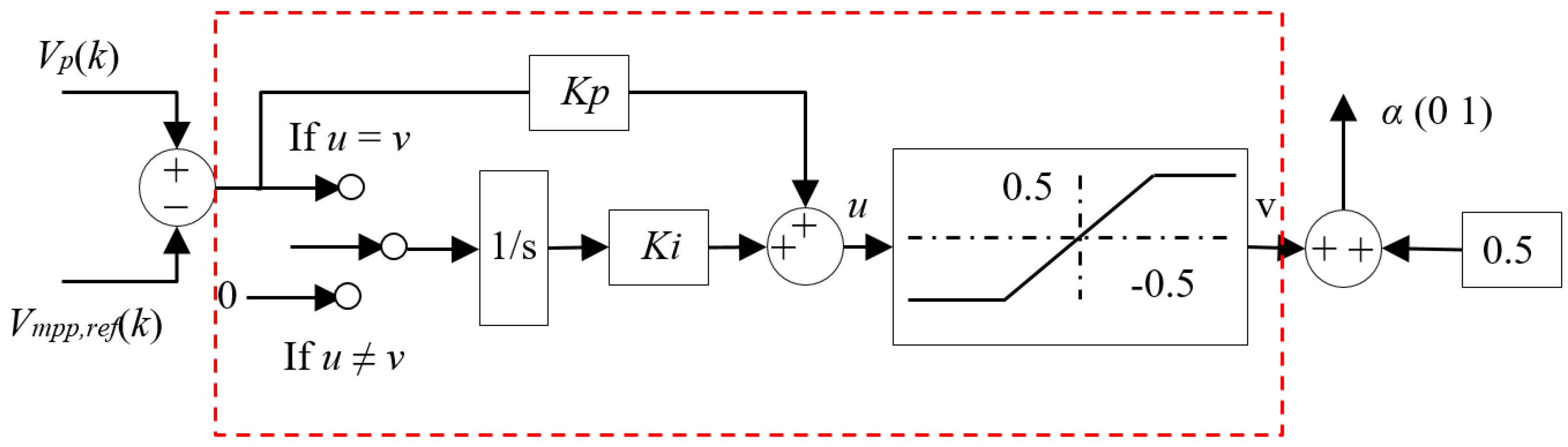
3.1.2. PI-1 Controller

The PI-1 controller with an anti-windup block (refer to [32]) serves as the second sub-controller of the system. Figure 4 and Figure 8 show detailed schematics of the controller.

3.2. DC Link Voltage Regulator Module

According to Figure 3, the objective of the DC link voltage regulator is to determine an appropriate value of the reference grid current I g r e f used for the current controller module. We note that the ultimate goal here is to make the DC link voltage V D C reach its desired value V D C r e f once the actual grid current I g is well regulated to its reference I g r e f [7,8] by the proposed current controller module using the LQR technique, which will be shown in detail in Section 3.3. In existing studies, a conventional PI controller has often been used to generate the reference grid current I g r e f from the DC link voltage difference e V d c = V D C r e f V D C , as shown in the upper left part of Figure 9. Nevertheless, it is difficult to manually choose and tune optimal values for the coefficients of the PI-2 controller due to the high nonlinearity of the grid-connected PV system, including a LCL output filter. Furthermore, the response of the conventional PI-2 controller usually has fairly large overshoot in the transient state and achieves the steady state in a relatively slow manner. Thus, this paper proposes a novel hybrid control scheme for the DC link voltage regulator module using another FLC (named FLC-2) as depicted in Figure 9 to overcome the above-mentioned drawbacks of the traditional PI-2 controller and remarkably enhance the response time.
Firstly, the theoretical relation between the output power of the DC-AC inverter supplied to the grid P A C and the output power of the PV array P P can be expressed as follows:
P A C = η D C A C × P D C l i n k = η D C A C × ( η D C D C × P P ) = η E x p × P P
where:
  • η D C D C —the efficiency of the buck-boost DC-DC converter can be estimated theoretically as a ratio value of the DC link power P D C l i n k and the output power of PV array P P ;
  • η D C A C —the efficiency of the DC-AC inverter can be estimated theoretically as a ratio value of the output power of the inverter P A C and the DC link power P D C l i n k ;
  • η E x p = η D C D C × η D C A C —the overall efficiency of the grid-connected PV system.
Equation (7) can be written as:
V g I g ( cos θ g ) = η E x p P P
here cosθg is the PF of the PV system, Vg is the rms value of the grid voltage, and Ig is the rms value of the grid current. In the normal operation of the grid, the rms value of the grid voltage is often larger than zero, meaning that Vg > 0 V.
Hence,
I g = η E x p P P V g ( cos θ g )  
When the PF = 1, the grid current will reach the following value.
I g = η E x p P P / V g
However, the actual overall efficiency η E x p depends not only on the PF, but also on other component parameters of the DC-DC buck-boost converter and the DC-AC inverter, as well as the operating conditions of the PV system (e.g., the PV power, temperature, input voltage, and so forth); as a result, it is difficult to accurately estimate a particular value for η E x p . We note that Equations (7)–(10) are only explanations of the theoretical relations among the parameters η E x p , P P , P A C , I g , and V g , which are used as the reference basis for introducing and calculating a new “virtual efficiency” η e x p v i r in our proposed hybrid control scheme for the DC link voltage regulator module, as depicted in Figure 9. Hence, the calculated value of the “virtual efficiency” η e x p v i r in this figure and (11) is not the actual value of the overall efficiency of the PV system η E x p in (7). In this study, we calculate the “virtual efficiency” value η e x p v i r instead of estimating the actual overall efficiency η E x p .
To fulfill the above goal, the FLC-2 is designed to frequently update a suitable value for the “virtual efficiency” η e x p v i r ( k ) in real-time, as described in (11) and Figure 9. Then, from (10), an additional value I g F L C for adjusting the reference grid current I g r e f can be computed as I g F L C ( k ) = η e x p v i r ( k ) × P P ( k ) / V g ( k ) , as shown in the right part of Figure 9. Finally, this computed additional value I g F L C ( k ) is used to effectively compensate for the output of the conventional PI-2 controller I g P I ( k ) to appropriately determine the reference grid current I g r e f ( k ) , as presented in the upper right part of Figure 9; in detail, I g r e f ( k ) = I g P I ( k ) + I g F L C ( k ) . The key aims of I g F L C ( k ) generated by our proposed control scheme using the FLC-2 are to significantly improve the response time for updating a suitable value for the reference current I g r e f ( k ) and to elevate the effectiveness of the conventional PI-2 controller against effects caused by the high nonlinearity of the PV system.
In fact, using the proposed current controller module (refer to Figure 3 and Section 3.3), when the grid current I g ( k ) is regulated to its reference I g r e f ( k ) suitably generated by the designed PI-Fuzzy hybrid control scheme (see Figure 9), the DC link voltage V D C achieves its desired value V D C r e f [7,8]. This means that both the error values of the DC link voltage ( e V d c in Figure 9) and the grid current in (14) and (15) are considered and regulated by the proposed complete control system, as given in the lower part of Figure 3.
The designed FLC-2 has two inputs and one output.
The two inputs are:
  • e V d c (k)—error between desired and present DC link voltage;
  • d e V d c (k)—change in error.
The output is:
  • Δ η (k)—step in efficiency, added to the “virtual efficiency” η e x p v i r to reach the desired value:
    η e x p v i r ( k ) = η e x p v i r ( k 1 ) + Δ η ( k )  
The two inputs are:
e V d c ( k ) = V D C r e f V D C ( k )
d e V d c ( k ) = e V d c ( k ) e V d c ( k 1 )  
All the inputs have the same number of linguistic variables, specifically seven; the range is [−20;20]: NL—Negative Large, NM—Negative Medium, NS—Negative Small, ZE—Zero, PS—Positive Small, PM—Positive Medium, PL—Positive Large
The output ΔȠ(k) has nine linguistic variables, and they range from [−1;1]: NL—Negative Large, NM—Negative Medium, NS—Negative Small, NZ—Negative Zero, ZE—Zero, PZ—Positive Zero, PS—Positive Small, PM—Positive Medium, PL—Positive Large. As a result, there are 49 fuzzy rules formed in the FLC-2.
All the association rules of the FLC-2 are presented in Table 5, while the membership functions of the inputs and output can be referred to in [28]. To interpret the fuzzy rules in Table 5, we can analyze and evaluate some sample cases as follows. Firstly, when deVdc(k) is NL and eVdc(k) is PL, the output of the fuzzy controller Δ η (k) should be ZE since the tendency of the DC-link voltage Vdc(k) is automatically approaching its reference value. On the other hand, when deVdc(k) is ZE and eVdc(k) is NL, it means that Vdc(k) is much smaller than its reference value; thus, the output Δ η (k) should be PL to force Vdc(k) to rapidly move to the desired value. Furthermore, when deVdc(k) is ZE and eVdc(k) is PS, it means that Vdc(k) is marginally larger than its reference value; hence, the output Δ η (k) should be NS to slightly decrease Vdc(k) to its desired value without oscillation at the steady state. In general, the other fuzzy rules in Table 5 can be appropriately explained with a similar deductive technique.

3.3. Current Controller Module

In this section, the current controller is designed by an optimal control method. Firstly, from (2), we have the following dynamic model,
{ x ˙ 4 = R L x 4 1 L x 5 + u L     x ˙ 5 = 1 C x 4 1 C x 6                           x ˙ 6 = 1 L g x 5 R g L g x 6 1 L g V g
The main purpose of the current controller is to make the grid current ig (i.e., x6) converge to its reference x6ref. Then, from the third equation of (14), the error dynamics of x6 and the reference for x5 (i.e., x5ref) can be derived as,
x ˙ 6 x ˙ 6 r e f = 1 L g ( ( x 5 x 5 r e f ) + x 5 r e f ) R g L g ( ( x 6 x 6 r e f ) + x 6 r e f ) 1 L g V g
Thus, we have
x ˜ ˙ 6 = 1 L g x ˜ 5 R g L g x ˜ 6 1 L g x 5 r e f
where x5ref is determined by
x 5 r e f = R g x 6 r e f + v g + x ˙ 6 r e f L g
Similarly, with x5ref achieved from (17), combined with the second equation of (14),
x ˙ 5 x ˙ 5 r e f = 1 C ( ( x 4 x 4 r e f ) + x 4 r e f ) 1 C ( ( x 6 x 6 r e f ) + x 6 r e f )
then
x ˜ ˙ 5 = 1 C x ˜ 4 1 C x ˜ 6
where
x 4 r e f = x 6 r e f + x ˙ 5 r e f C f
From x5ref and x4ref, obtained in (17) and (20), respectively, the first equation of (14) can be rewritten as
x ˜ ˙ 4 = R L x ˜ 4 R L x 4 r e f 1 L x ˜ 5 1 L x 5 r e f x ˙ 4 r e f + 1 L u 1 + 1 L u 2
Hence, we have
x ˙ 4 = R L x ˜ 4 1 L x ˜ 5 + 1 L u 1
where
u 2 = R x 4 r e f + x 5 r e f + L x ˙ 4 r e f
Here, we decompose the control input u into two terms: u1 and u2; in detail, u1 is used for feedback control to stabilize the error dynamics, whereas u2 is the compensating term used to compensate for the offset in the reference tracking problem. Finally, the error dynamics of (15) are achieved by combining (22), (19), and (16), as follows:
[ x 4 x 5 x 6 ] = [ R g L g                         1 L g           0 1 L                         0                 1 C   0                   1 L         R L ] + [ 0 0 1 L ] u 1
Equation (24) is rewritten in the following form:
x ˙ = A x + B u 1
Consider the following cost function:
J ( x , u ) = 0 x T Q x + u 1 T Q u 1
where Q ≥ 0 and R > 0 are the weighting matrices with appropriate dimensions; that is, 3 × 3 and a scalar, respectively. After that, this cost function is minimized by the following control law:
u 1 = K x = R 1 B T P x
where K is the controller gain matrix, and P is the positive definite solution of the algebraic Riccati equation as follows
P A + A T P P B R 1 B T P + Q = 0
Typically, Q is chosen to be diagonal:
Q = [ q 1         0             0     0           q 2           0     0               0           q 3   ]
where its elements and R can be selected by the following criteria,
q i = 1 t s i ( x i m a x ) 2 ,   R = 1 ( u 1 m a x ) 2 ,   p > 0
In (30), ximax is the |xi| constraint, uimax is the |ui| constraint, and tsi is the required settling time of xi.

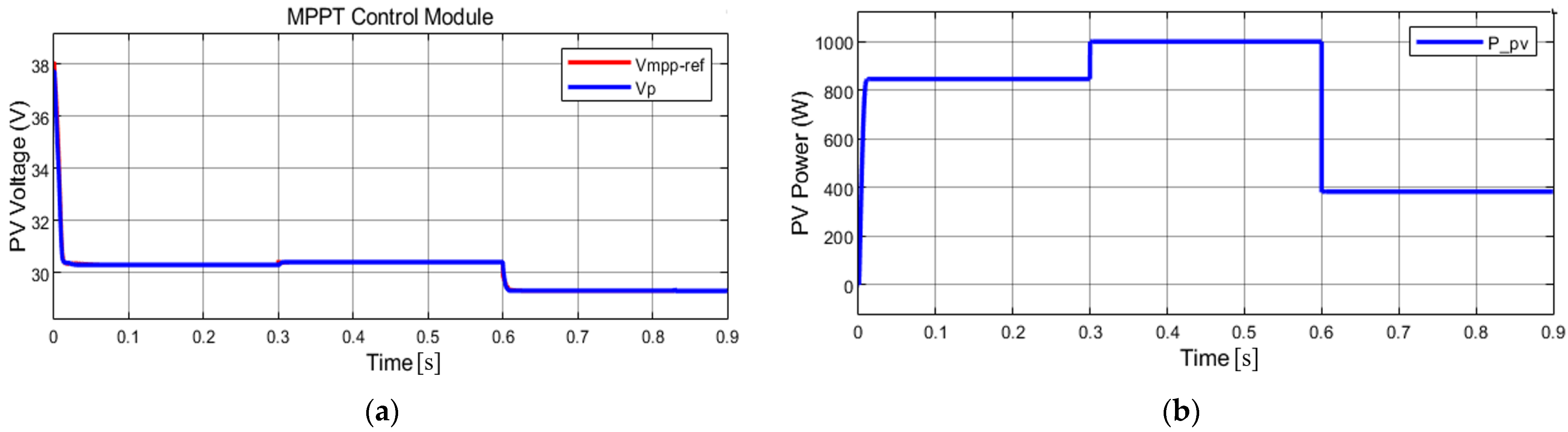
4. Simulation Results

The simulation performed in MATLAB/Simulink and all related parameters of the considered PV system can be referred to in [28]. The results with the designed LQR control are illustrated in Figure 10, Figure 11, Figure 12 and Figure 13, in which the time unit in the horizontal axis is second.

4.1. Simulation 1: Constant Module Temperature

This case considers when the PV module temperature is constant at 25 °C. Irradiation starts from 850 W/m2 at a time from 0 s to 0.3 s, then it becomes 1000 W/m2 from 0.3 s to 0.6 s and finally becomes 400 W/m2 from 0.6 s to 0.9 s. Figure 10 shows that the results of the voltage Vp of the PV array are close to the reference values for the MPPT. The obtained output powers of the PV array are 847 W, 998 W, and 385 W, which match to the reference data provided in Table 1. Thus, this means that the power loss is small in this test.
The DC-link voltages correspond to each other in Figure 11. Furthermore, the grid current is equal to the reference values. Finally, it was shown and proven that the voltage and current of the grid are in phase, which means that the power factor of the grid-connected PV system is nearly unity.

4.2. Simulation 2: Constant Solar Irradiation

In the second case, solar irradiation is constant at 1000 W/m2, but the module temperature is varying. From t = 0 s to 0.3 s temperature is 25 °C, next, at 0.3 s the temperature is 45 °C, and lastly, at 0.3 s the temperature is 30 °C. According to Figure 12, the performance of the panel is 30.38 V/1000 W, 27.92 V/912.1 W, and 29.76 V/978.8 W, which is highly close to the values represented in Table 1. Despite the module temperature change, VDC matched its reference at all times. In addition, the RMS value of Ig is maintained according to the reference trend, as presented in Figure 13. The phases of the grid voltage and current match, which means that the system’s power factor is unity.

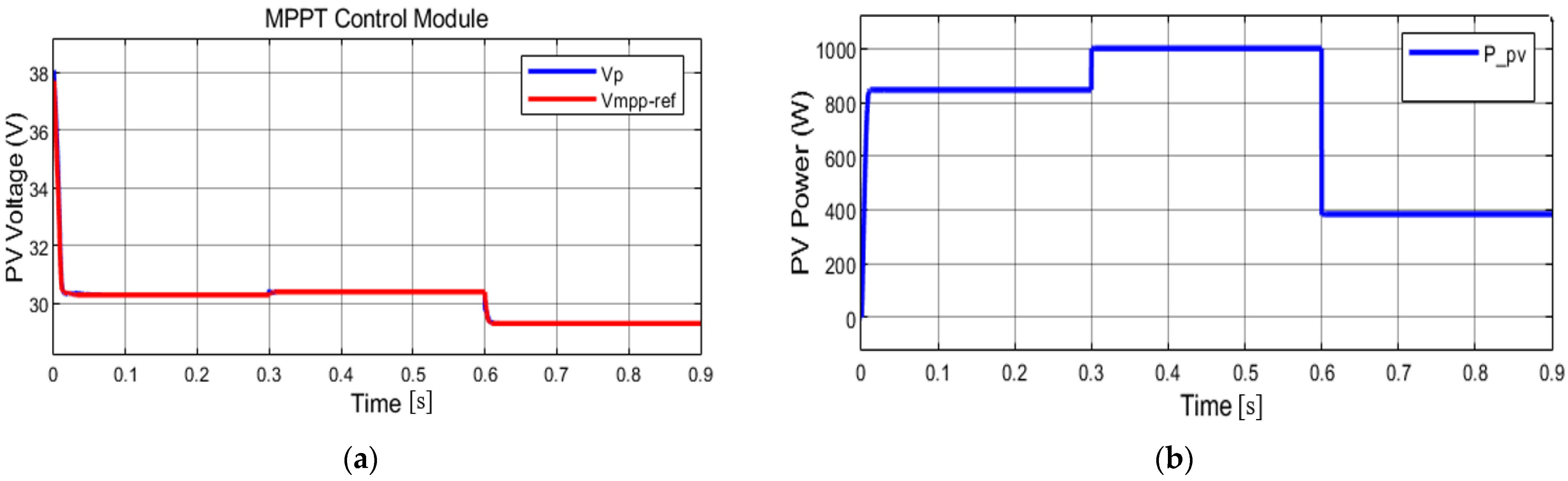
5. Comparison between LQR and Backstepping Approaches

This research suggests the suitable combination of an LQR and fuzzy control for grid-connected PV systems. To show the effectiveness of the provided technique, it is important to make comparisons between some other methods, such as photovoltaic grid-connected systems using fuzzy logic and backstepping approaches [28] (see this reference paper for the specific details of simulations). Figure 14, Figure 15, Figure 16 and Figure 17 present the simulation results of fuzzy control and the backstepping approach for a grid-connected photovoltaic system with the module temperature (Figure 14 and Figure 15), and then with constant solar irradiation (Figure 16 and Figure 17), in which the time unit in the horizontal axis is seconds. The obtained simulation results should be compared to those of the above-mentioned method. Specifically, the results in Figure 11 and Figure 13 should be compared with those in Figure 15 and Figure 17, respectively. We can see that both the control methods have good results.

5.1. Simulation 1: Constant Module Temperature

It is obvious that the simulation results of the MPPT parts in both the cases are the same since the main changes were not related to the MPPT controller, but to the LQR. Thus, the behaviors shown in Figure 10 and Figure 14 are same; the performances presented in Figure 12 and Figure 16 are also similar. Comparing the DC link voltage regulator module and the current controller module in both the cases, it can be clearly seen that the LQR case reacts to the changes in the module temperature and irradiation faster; in other words, the settling time of the LQR technique is lower compared to the backstepping method. Moreover, the LQR is robust when faced with different temperature and irradiation changes, which makes this technique preferable. In addition, in the case of the backstepping method, overshooting of the signal was observed, which significantly degrades the output and overall efficiency of the considered PV system. Furthermore, the response speed of the designed LQR is faster; consequently the rise time and peak time of the LQR are lower than those of the backstepping approach.

5.2. Simulation 2: Constant Solar Irradiation

In addition, the fuzzy-based INC-MPPT controller (see Figure 3, Figure 4, Figure 5, Figure 6 and Figure 7 and Table 4) in this paper is improved from our past method [33], with significant modifications in the pre-scaling module Gp(k) for increasing the sensitivity of the slope Sp(k), in the fuzzy association rules for boosting the speed of searching the MPP, and in the control parameter values, which are designed and tuned to be more suitable for grid-connected PV systems with the LCL output filter. The detailed analysis and evaluation of the effectiveness of the prior related MPPT method for a small stand-alone PV system in various simulations and experiments can be referred to in Sections 4 and 5 of our past work [33], in which cases of partial shadow on the PV array were also investigated in experiments. Moreover, the influence of the module temperature on the performance of the stand-alone PV system and MPPT controller can be found in Sections 2.2 and 4.3 of the prior study [33]. In fact, our present paper proposes a complete control solution for grid-connected single-phase PV systems including the LCL output filter based on fuzzy control and LQR techniques with multiple objectives as described in Section 1 and Section 3 above; thus, it is noted that the separate assessment of the MPPT controller compared to other MPPT systems is out the scope of this study.
Due to substantial differences in configurations of considered PV systems and control objectives between this study and other existing works, it seems inappropriate and difficult to directly compare the detailed effectiveness of the proposed control scheme in this research to that of other studies. Therefore, we have only performed the detailed comparison of the current controller module using the LQR method proposed in the present paper with our past work using the backstepping approach [28] for evaluation, as described in Section 5 above. Moreover, for further reference, the current controller module using the LQR technique in this paper is briefly compared with the PID-fuzzy hybrid controller introduced in our other study [34], as represented in Table 6.
In this grid-connected PV system using a DC-AC inverter and LCL output filter, due to parasitic capacitance and grounding resistance, the issues of common mode (CM) voltage and leakage current may become significant if the design and control of the inverter and LCL filter are not appropriate [35,36]. As presented in other existing studies [37,38], the issues of CM voltage and leakage current in grid-connected PV systems can be effectively investigated and reduced using various techniques such as improved PWM methods, modified topologies of PV inverters with complementary switches [37], design and implementation of CM filters [38,39], active damping control approaches [40], and so forth. On the other hand, our paper focuses on developing a complete control scheme for grid-connected single-phase PV systems including an LCL filter based on fuzzy logic and an LQR method with three key goals comprising the MPPT, DC link voltage regulation, and injection of the PV power into the grid with a unity PF. Hence, it should be noted that the assessment and reduction of the CM voltage and leakage current are beyond the scope of the present paper; these issues will be thoroughly considered in our future work.

6. Conclusions

Based on fuzzy control and an LQR, this study provides a comprehensive control solution for grid-connected single-phase PV systems. In terms of improving the quality of controller methods, this work represents a substantial extension and enhancement of our past research. For grid-connected solar systems, the suggested approach is an LQR suitably combined with fuzzy control, in which the design procedures of all the controllers are also described in detail. The major novelty of this study is to demonstrate and verify that the newly proposed approach is more successful in different aspects by comparing our past and present control methods. The LQR technique’s major benefit is its ability to react quickly to unexpected changes in the system, such as changes in module temperature and solar irradiation. In other words, the systems achieve their settling period sooner, which is necessary to steady the output behavior.
Furthermore, as compared to the backstepping approach, the LQR method is more resistant to various changes in weather conditions. The backstepping approach also has the greater overrun, which has a detrimental effect on the efficiency of the investigated PV system. As previously stated, the LQR has the quicker response speed, making this type of controller more desirable. These are the major contributions of our present work as compared to the earlier research. Moreover, the results of simulations under different weather circumstances were compared to theoretical ones, indicating that the proposed system can cope with variations in weather parameters well. It was also demonstrated that abrupt changes in weather factors had no significant effects on the proposed control system’s performance.
In future work, intelligent models based on fuzzy control for effectively predicting PV power and load demand will be thoroughly studied and implemented to improve the effectiveness and quality of grid-connected solar energy systems, especially under adverse conditions such shaded solar PV modules.

Author Contributions

A.M. worked on all tasks; T.D.D. and N.G.M.T. worked on the methodology and supervised. All the authors participated in writing, editing, and review. All authors have read and agreed to the published version of the manuscript.

Funding

This work was supported by Nazarbayev University under the Faculty Development Competitive Research Grant Program (FDCRGP), Grant No. 11022021FD2924.

Data Availability Statement

Not applicable.

Conflicts of Interest

The authors declare no conflict of interest.

References

  1. Torquato, R.; Arguello, A.; Freitas, W. Practical Chart for Harmonic Resonance Assessment of DFIG-Based Wind Parks. IEEE Trans. Power Deliv. 2020, 35, 2233–2242. [Google Scholar] [CrossRef]
  2. Thao, N.G.M.; Uchida, K.; Kofuji, K.; Jintsugawa, T.; Nakazawa, C. A comprehensive analysis study about harmonic resonances in megawatt grid-connected wind farms. In Proceedings of the 2014 International Conference on Renewable Energy Research and Application (ICRERA), Milwaukee, WI, USA, 19–22 October 2014; pp. 387–394. [Google Scholar]
  3. Alajmi, B.N.; Ahmed, K.H.; Finney, S.J.; Williams, B.W. Fuzzy-Logic-Control Approach of a Modified Hill-Climbing Method for Maximum Power Point in Microgrid Standalone Photovoltaic System. IEEE Trans. Power Electron. 2011, 26, 1022–1030. [Google Scholar] [CrossRef]
  4. Kottas, T.L.; Boutalis, Y.S.; Karlis, A.D. New Maximum Power Point Tracker for PV Arrays Using Fuzzy Controller in Close Cooperation with Fuzzy Cognitive Networks. IEEE Trans. Energy Convers. 2006, 21, 793–803. [Google Scholar] [CrossRef]
  5. Hamidia, F.; Abbadi, A.; Boucherit, M.S. Maximum Power Point Tracking Control of Photovoltaic Generation Based on Fuzzy Logic. In International Conference in Artificial Intelligence in Renewable Energetic Systems; Springer: Cham, Switzerland, 2018; pp. 197–205. [Google Scholar] [CrossRef]
  6. Menniti, D.; Pinnarelli, A.; Brusco, G. Implementation of a novel fuzzy-logic based MPPT for grid-connected photovoltaic generation system. In Proceedings of the 2011 IEEE Trondheim PowerTech, Trondheim, Norway, 19–23 June 2011. [Google Scholar] [CrossRef]
  7. Yang, B.; Li, W.; Zhao, Y.; He, X. Design and Analysis of a Grid-Connected Photovoltaic Power System. IEEE Trans. Power Electron. 2009, 25, 992–1000. [Google Scholar] [CrossRef]
  8. El Fadil, H.; Giri, F.; Guerrero, J. Grid-connected of photovoltaic module using nonlinear control. In Proceedings of the 2012 3rd IEEE International Symposium on Power Electronics for Distributed Generation Systems (PEDG), Aalborg, Denmark, 25–28 June 2012; pp. 119–124. [Google Scholar] [CrossRef] [Green Version]
  9. Wai, R.-J.; Wang, W.-H. Grid-Connected Photovoltaic Generation System. IEEE Trans. Circuits Syst. I Regul. Pap. 2008, 55, 953–964. [Google Scholar] [CrossRef]
  10. Reddy, D.; Ramasamy, S. A fuzzy logic MPPT controller based three phase grid-tied solar PV system with improved CPI voltage. In Proceedings of the 2017 Innovations in Power and Advanced Computing Technologies (I-PACT), Vellore, India, 21–22 April 2017; pp. 1–6. [Google Scholar] [CrossRef]
  11. Kumar, J.; Rathor, B.; Bahrani, P. Fuzzy and P amp; O MPPT techniques for stabilized the efficiency of solar PV system. In Proceedings of the 2018 International Conference on Computing, Power and Communication Technologies (GUCON), Greater Noida, India, 28–29 September 2018; pp. 259–264. [Google Scholar] [CrossRef]
  12. Kumar, B.P.; Winston, D.P.; Christabel, S.C.; Venkatanarayanan, S. Implementation of a switched PV technique for rooftop 2 kW solar PV to enhance power during unavoidable partial shading conditions. J. Power Electron. 2017, 17, 1600–1610. [Google Scholar] [CrossRef]
  13. Andrew-Cotter, J.; Uddin, M.N.; Amin, I.K. Particle swarm optimization based adaptive neuro-fuzzy inference system for MPPT control of a three-phase grid-connected photovoltaic system. In Proceedings of the 2019 IEEE International Electric Machines & Drives Conference (IEMDC), San Diego, CA, USA, 12–15 May 2019; pp. 2089–2094. [Google Scholar] [CrossRef]
  14. Arulkumar, K.; Palanisamy, K.; Vijayakumar, D. Recent advances and control techniques in grid connected Pv system—A review. Int. J. Renew. Energy Res. 2016, 6, 1037–1049. [Google Scholar]
  15. Mukundan, N.; Singh, Y.; Naqvi, S.B.Q.; Singh, B.; Pychadathil, J. Multi-Objective Solar Power Conversion System with MGI Control for Grid Integration at Adverse Operating Conditions. IEEE Trans. Sustain. Energy 2020, 11, 2901–2910. [Google Scholar]
  16. Alturki, F.A.; Omotoso, H.O.; Al-Shamma’A, A.A.; Farh, H.M.H.; Alsharabi, K. Novel Manta Rays Foraging Optimization Algorithm Based Optimal Control for Grid-Connected PV Energy System. IEEE Access 2020, 8, 187276–187290. [Google Scholar] [CrossRef]
  17. Blaabjerg, F.; Teodorescu, R.; Liserre, M.; Timbus, A.V. Overview of Control and Grid Synchronization for Distributed Power Generation Systems. IEEE Trans. Ind. Electron. 2006, 53, 1398–1409. [Google Scholar] [CrossRef] [Green Version]
  18. Teodorescu, R.; Blaabjerg, F.; Liserre, M.; Loh, P.C. Proportional-resonant controllers and filters for grid-connected voltage-source converters. IET Proc. Electr. Power Appl. 2006, 153, 750–762. [Google Scholar] [CrossRef] [Green Version]
  19. Wu, G.R.; Dewan, R.; Slemon, S.B. Analysis of a PWM AC to DC Voltage Source Converter under the Predicted Current Control with a Fixed Switching Frequency. IEEE Trans. Ind. Appl. 1991, 27, 756–764. [Google Scholar] [CrossRef]
  20. Zhang, K.; Kang, Y.; Xiong, J.; Chen, J. Direct repetitive control of SPWM inverter for UPS purpose. IEEE Trans. Power Electron. 2003, 18, 784–792. [Google Scholar] [CrossRef]
  21. Singh, B.; Jain, V. TOCF Based Control for Optimum Operation of a Grid Tied Solar PV System. IEEE Trans. Energy Convers. 2020, 35, 1171–1181. [Google Scholar] [CrossRef]
  22. Shan, Y.; Hu, J.; Guerrero, J.M. A Model Predictive Power Control Method for PV and Energy Storage Systems with Voltage Support Capability. IEEE Trans. Smart Grid 2019, 11, 1018–1029. [Google Scholar] [CrossRef]
  23. Manoharan, M.S.; Ahmed, A.; Park, J.-H. An Improved Model Predictive Controller for 27-Level Asymmetric Cascaded Inverter Applicable in High-Power PV Grid-Connected Systems. IEEE J. Emerg. Sel. Top. Power Electron. 2019, 8, 4395–4405. [Google Scholar] [CrossRef]
  24. Mahfuz-Ur-Rahman, A.M.; Islam, R.; Muttaqi, K.M.; Sutanto, D. Model Predictive Control for a New Magnetic Linked Multilevel Inverter to Integrate Solar Photovoltaic Systems with the Power Grids. IEEE Trans. Ind. Appl. 2020, 56, 7145–7155. [Google Scholar] [CrossRef]
  25. Mansour, A.M.; Arafa, O.M.; Marei, M.I.; Abdelsalam, I.; Aziz, G.A.A.; Sattar, A.A. Hardware-in-the-Loop Testing of Seamless Interactions of Multi-Purpose Grid-Tied PV Inverter Based on SFT-PLL Control Strategy. IEEE Access 2021, 9, 123465–123483. [Google Scholar] [CrossRef]
  26. Verma, A.; Singh, B. CAPSA Based Control for Power Quality Correction in PV Array Integrated EVCS Operating in Standalone and Grid Connected Modes. IEEE Trans. Ind. Appl. 2020, 57, 1789–1800. [Google Scholar] [CrossRef]
  27. Sarita, K.; Kumar, S.; Vardhan, A.S.S.; Elavarasan, R.M.; Saket, R.K.; Shafiullah, G.M.; Hossain, E. Power Enhancement with Grid Stabilization of Renewable Energy-Based Generation System Using UPQC-FLC-EVA Technique. IEEE Access 2020, 8, 207443–207464. [Google Scholar] [CrossRef]
  28. Thao, N.G.M.; Uchida, K. Control the photovoltaic grid-connected system using fuzzy logic and backstepping approach. In Proceedings of the 2013 9th Asian Control Conference ASCC, Istanbul, Turkey, 23–26 June 2013; pp. 1–8. [Google Scholar] [CrossRef]
  29. Katir, H.; Abouloifa, A.; Noussi, K.; Lachkar, I.; El Aroudi, A.; Aourir, M.; El Otmani, F.; Giri, F. Fault Tolerant Backstepping Control for Double-Stage Grid-Connected Photovoltaic Systems Using Cascaded H-Bridge Multilevel Inverters. IEEE Control Syst. Lett. 2021, 6, 1406–1411. [Google Scholar] [CrossRef]
  30. Liserre, M.; Blaabjerg, F.; Hansen, S. Design and Control of an LCL-Filter-Based Three-Phase Active Rectifier. IEEE Trans. Ind. Appl. 2005, 41, 1281–1291. [Google Scholar] [CrossRef]
  31. Sun, W.; Chen, Z.; Wu, X. Intelligent optimize design of LCL filter for three-phase voltage-source PWM rectifier. In Proceedings of the 2009 IEEE 6th International Power Electronics and Motion Control Conference, Wuhan, China, 17–20 May 2009; pp. 970–974. [Google Scholar] [CrossRef]
  32. Li, X.-L.; Park, J.-G.; Shin, H.-B. Comparison and Evaluation of Anti-Windup PI Controllers. J. Power Electron. 2011, 11, 45–50. [Google Scholar] [CrossRef] [Green Version]
  33. Thao, N.G.M.; Uchida, K.; Nguyen-Quang, N. An Improved Incremental Conductance-Maximum Power Point Tracking Algorithm Based on Fuzzy Logic for Photovoltaic Systems. SICE J. Control. Meas. Syst. Integr. 2014, 7, 122–131. [Google Scholar] [CrossRef] [Green Version]
  34. Thao, N.G.M.; Dat, M.T.; Binh, T.C.; Phuc, N.H. PID-fuzzy logic hybrid controller for grid-connected photovoltaic inverters. In Proceedings of the International Forum on Strategic Technology, Ulsan, Korea, 13–15 October 2010; pp. 140–144. [Google Scholar] [CrossRef]
  35. Zeb, K.; Khan, I.; Uddin, W.; Khan, M.A.; Sathishkumar, P.; Busarello, T.D.C.; Ahmad, I.; Kim, H.J. A Review on Recent Advances and Future Trends of Transformerless Inverter Structures for Single-Phase Grid-Connected Photovoltaic Systems. Energies 2018, 11, 1968. [Google Scholar] [CrossRef] [Green Version]
  36. Figueredo, R.S.; De Carvalho, K.C.M.; Ama, N.R.N.; Matakas, L. Leakage current minimization techniques for single-phase transformerless grid-connected PV inverters—An overview. In Proceedings of the 2013 Brazilian Power Electronics Conference, Gramado, Brazil, 27–31 October 2013; pp. 517–524. [Google Scholar] [CrossRef]
  37. Hedayati, M.H.; John, V. EMI and ground leakage current reduction in single-phase grid-connected power converter. IET Power Electron. 2017, 10, 938–944. [Google Scholar] [CrossRef]
  38. Figueredo, R.S.; Matakas, L. Integrated Common and Differential Mode Filter With Capacitor-Voltage Feedforward Active Damping for Single-Phase Transformerless PV Inverters. IEEE Trans. Power Electron. 2019, 35, 7058–7072. [Google Scholar] [CrossRef]
  39. Liu, Y.; Lai, C.-M. LCL Filter Design with EMI Noise Consideration for Grid-Connected Inverter. Energies 2018, 11, 1646. [Google Scholar] [CrossRef] [Green Version]
  40. Niyomsatian, K.; Vanassche, P.; Gyselinck, J.J.C.; Sabariego, R.V. Active-Damping Virtual Circuit Control for Grid-Tied Converters with Differential-Mode and Common-Mode Output Filters. IEEE Trans. Power Electron. 2020, 35, 7583–7595. [Google Scholar] [CrossRef]
Figure 1. PV single-phase grid-connected system.
Energies 15 01286 g001
Figure 2. Power obtained from PV panels for different (a) solar radiation values and (b) module temperature values.
Energies 15 01286 g002
Figure 3. System schematics in detail.
Energies 15 01286 g003
Figure 4. MPPT controller module schematics.
Energies 15 01286 g004
Figure 5. FLC-1 structure.
Energies 15 01286 g005
Figure 6. INC-MPPT algorithm with fuzzy logic.
Energies 15 01286 g006
Figure 7. PV panel power–voltage (P-V) curve.
Energies 15 01286 g007
Figure 8. PI-1 controller in detail.
Energies 15 01286 g008
Figure 9. Proposed PI-fuzzy hybrid control scheme, where g3, g4 and g5 are design coefficients.
Energies 15 01286 g009
Figure 10. MPPT module performance for constant temperature: (a) PV voltage; (b) PV output power.
Energies 15 01286 g010
Figure 11. DC link voltage regulator module and current controller module performances with the LQR method for constant temperature case: (a) DC link voltage; (b) grid current magnitude; (c) grid voltage waveform Vg (V) and current waveform where Gain is 10 × I g   ( A ) .
Energies 15 01286 g011
Figure 12. MPPT module performance for constant solar irradiation: (a) PV voltage; (b) PV output power.
Energies 15 01286 g012
Figure 13. DC link voltage regulator module and current controller module performances with the LQR for constant solar irradiation case: (a) DC link voltage; (b) grid current magnitude; (c) grid voltage waveform Vg (V) and current waveform where gain is 10 × I g   ( A ) .
Energies 15 01286 g013
Figure 14. MPPT module performance in case with the backstepping approach for constant temperature: (a) PV voltage; (b) PV output power.
Energies 15 01286 g014
Figure 15. DC link voltage regulator module and current controller module performances with backstepping approach for constant temperature case: (a) DC link voltage; (b) grid current magnitude; (c) grid voltage waveform Vg (V) and current waveform where gain is 10 × I g   ( A ) .
Energies 15 01286 g015
Figure 16. MPPT module performance in case with the backstepping approach for constant solar irradiation: (a) PV voltage; (b) PV output power.
Energies 15 01286 g016
Figure 17. DC link voltage regulator module and current controller module performances with backstepping approach for constant solar irradiation case: (a) DC-link voltage; (b) grid current magnitude; (c) grid voltage waveform Vg (V) and current waveform where gain is 10 × I g   ( A ) .
Energies 15 01286 g017
Table 1. Power and Voltage at Maximum Power Points.
MPPsM1M2M3/M4M5M6
Vp (V)29.330.3230.429.828.04
PP,panel (W)95.9211.7250244.8225.7
PP,array (W)383.6846.81000979.2912.8
Table 2. Variables.
Table 2. Variables.
VariableSymbol in Figure 1Averaged Variable in (1)
PV array voltageVpx1
Current through the inductor L1iL1x2
DC link voltageVDCx3
Input current of the LCL filterifx4
Voltage on the capacitor CfVCfx5
RMS value of the electric grid currentigx6
Control signal of the non-inverting buck-boost DC-DC converterαp
{0,1}
α
(0,1)
Control signal of the single-phase DC-AC inverterβp
{−1,0,1}
β
[−1,1]
PV array currentIpĪp
RMS value of the electric grid voltageVgVg
Table 3. Switching module operation.
If the Input Is |AP(k)|If the Input Is |dIP(k)|
|AP(k)| > 0.1|AP(k) ≤ 0.1g2 = 1 (where every value of |dIP(k)|)
g2 = 0.25g2 = 0.1
Table 4. Fuzzy association rules for FLC-1.
Vadd(k)|Ap(k)| or |dIp(k)|
VSSMMELAVL
ΔV(k−1)VSZEPZPSPLPL
SMNZZEPZPMPL
MENSNZZEPSPM
LANMNSNZPZPS
VLNLNMNSZEPZ
Table 5. Fuzzy association rules for FLC-2.
Δη(k)eVdc(k)
NLNMNSZEPSPMPL
deVdc(k)NLPUPUPLPLPMPSZE
NMPUPUPLPMPSZENS
NSPUPLPMPSZENSNM
ZEPLPMPSZENSNMNL
PSPMPSZENSNMNLNU
PMPSZENSNMNLNUNU
PLZENSNMNLNLNUNU
Table 6. Comparison between the proposed current controller module and the previously introduced PID-fuzzy controller in [34].
Control MethodsThe Current Controller Module Using the LQR in This PaperThe Introduced PID-Fuzzy Hybrid Controller in [34]
Design and computational complexity
-
Fairly simple design based on an optimal control method using the algebraic Riccati equation (see Section 3.3)
-
Includes three separate FLCs for controlling gains Kp, KI, and KD, in which each FLC consists of 49 association rules.
Field of application in power systems
-
For a complete single-phase grid-connected PV system including the LCL output filter with the consideration of DC link voltage regulation.
-
For a simple single-phase grid-connected PV system including the L output filter without the consideration of DC link voltage regulation.
Control objectives,
performance, and effectiveness
-
Can well regulate the grid current with a unity power factor and DC link voltage under different operating conditions of the PV system.
-
Very fast response, and small overshoot.
-
Has good efficacy and is robust faced with large variations in solar radiation and PV module temperature.
-
Theoretical analysis of stability of the LQR controller has been confirmed.
-
Can control the active and reactive power supplied to the grid with the step change of reference signals for the two powers.
-
Quick response and relatively small overshoot.
-
Has not yet been checked with large variations in solar radiation and PV module temperature.
-
Theoretical analysis of stability of the hybrid controller has not yet been performed.
Publisher’s Note: MDPI stays neutral with regard to jurisdictional claims in published maps and institutional affiliations.

