Article

An Online Data-Driven LPV Modeling Method for Turbo-Shaft Engines

Jiangsu Province Key Laboratory of Aerospace Power System, College of Energy and Power Engineering, Nanjing University of Aeronautics and Astronautics, Nanjing 210016, China
*
Author to whom correspondence should be addressed.
Energies 2022, 15(4), 1255; https://doi.org/10.3390/en15041255
Submission received: 7 December 2021 / Revised: 30 January 2022 / Accepted: 7 February 2022 / Published: 9 February 2022

Abstract

:
The linear parameter-varying (LPV) model is widely used in aero engine control system design. The conventional local modeling method is inaccurate and inefficient in the full flying envelope. Hence, a novel online data-driven LPV modeling method based on the online sequential extreme learning machine (OS-ELM) with an additional multiplying layer (MLOS-ELM) was proposed. An extra multiplying layer was inserted between the hidden layer and the output layer, where the hidden layer outputs were multiplied by the input variables and state variables of the LPV model. Additionally, the input layer was set to the LPV model’s scheduling parameter. With the multiplying layer added, the state space equation matrices of the LPV model could be easily calculated using online gathered data. Simulation results showed that the outputs of the MLOS-ELM matched that of the component level model of a turbo-shaft engine precisely. The maximum approximation error was less than 0.18%. The predictive outputs of the proposed online data-driven LPV model after five samples also matched that of the component level model well, and the maximum predictive error within a large flight envelope was less than 1.1% with measurement noise considered. Thus, the efficiency and accuracy of the proposed method were validated.

1. Introduction

The behavior of an aero engine can be described by a linear parameter-varying (LPV) model, which can approximate a nonlinear system or a time-varying linear system with a combination of linear time-invariant (LTI) models [1,2,3]. The parameters of LPV models are expressed as a function of the scheduling variables or the operating point variables, capturing the dynamic changes of the nonlinear system accurately [4,5]. The main advantage of LPV models is that they allow the application of well-established linear design techniques to complex nonlinear systems based on the linear matrix inequality [6,7] and linear quadric methods [8]. For example, the online optimization of model predictive control (MPC) or performance seeking control (PSC) can be reduced to a linear program or a quadratic program, thereby achieving high real-time property when an LPV model is used as a predictive model [9,10]. LPV models preserve the advantageous properties of LTI models, such as low modeling cost, while being able to represent a large class of nonlinear systems with high accuracy [11]. Therefore, the LPV model has been widely used in convex system controller design [12,13] and model-based approaches [14,15], such as robust control, fault diagnosis and optimal control.
The LPV and quasi-LPV identification method has attracted much attention in recent years [16,17,18]. Quasi- means that the scheduling parameters of the LPV model include system variables [19]. There are two main methods of LPV (or quasi-LPV) modeling which have been researched in the literature: the global method and the local method [20,21]. In the global method, the LPV model of the system can be derived from one experiment. Additionally, both control inputs and scheduling parameters are excited simultaneously in this experiment, which is not realizable in aero engine LPV modeling applications [20]. This is because the dynamic of the engine is a continuous function of the wide flying envelope and the various operation states, which can hardly be covered by finite-time experiments. Furthermore, the state variable of an aero engine is often directly selected as the scheduling parameter, which is dependent on control inputs and cannot be used to excite the system in a global modeling experiment. In the local method, a certain number of working states in the scheduling space are selected as the LPV model base point. A local LTI model is established at each point, and the LPV model is based on the interpolation of the local LTI systems [1,2,3,22,23]. The use of LTI models renders the local LPV modeling method simple and easily realized in complicated nonlinear systems.
However, for aero engines, it is difficult to build LTI models in the full flying envelope and variety of working states; also, the regularity of the parameters’ variation is poor [24,25]. The interpolation of the LTI parameters can be very complicated and time-consuming in the full envelope, and even fail to stabilize the system [26]. A common solution involves only modeling the aero engine at sea level with zero flying Mach numbers [27,28]. Models on other conditions are acquired through similarity transformation. Unfortunately, similarity transformation is carried out with many hypotheses which may not strictly hold in real operating states [29,30], especially for turbo-shaft engines. Therefore, the accuracy of the LPV model based on the similarity transformation may not satisfy the model-based control requirement of the turbo-shaft engine.
In recent years, data-driven methods have been employed as a powerful tool for LPV modeling since they can be carried out without mechanism models. In a data-driven modeling method, only the input, state and output trajectory information are used to identify the parameters [31]. The least square criterion and gradient descent algorithm are adopted to optimize the parameters of the LPV model [31,32,33]. A statistical approach was used in data-driven LPV system identification in [34]. However, the previously mentioned data-driven modeling methods are inefficient because they must be carried out offline [31,32,34] or carry online identification at the cost of reduced accuracy with the stochastic gradient descent algorithm. For aero engines, a more engaging, newly developed data-driven modeling method is the equilibrium manifold expansion (EME) model [35,36,37]. Differing from traditional LPV models of aero engines, the EME model considers the mapping between the equilibrium points of the engine and the scheduling parameters [36]. Thus, the EME can achieve high accuracy with less data. However, it can sometimes be difficult to find enough steady-state points to meet the needs of EME modeling, and then a similarity transformation must be conducted [37]. The similarity transformation may cause inaccuracies in the turbo-shaft engine. With the spread of intelligent technology, there have been efforts to build an LPV model by using support vector machines (SVM) [38,39], a promising approach to data-driven identification of LPV models [40]. Fényes et al. [41] presented a data-driven LPV modeling method for the control design of autonomous vehicle systems through machine learning, but it still required a reasonably large data set for training. Compared to the previous data-driven LPV modeling methods, the intelligent method can become more efficient by taking advantage of its online learning ability.
Hence, a novel online data-driven LPV (DD-LPV) modeling method for turbo-shaft engines based on a special neural network was proposed in this paper. It derived the DD-LPV model from an online sequential extreme learning machine (OS-ELM), with an extra multiplying layer (MLOS-ELM). It was able to achieve state space models at any operating point, static or dynamic, and modeling without the companion of the component-level model (CLM) of aero engines. Utilizing the online DD-LPV model derived by MLOS-ELM, a state space model was generated at every sample period based on the instant online gathered data, which made this model represent the current property of the individual engine accurately in any flight condition.
Compared with existing studies, the main contribution of this paper can be summarized as follows: (1) A special structure OS-ELM named MLOS-ELM was proposed in order to build a state space model directly and conveniently in the form of an artificial neural network. With the multiplying layer added, the neural network model and the LPV model were linked closely in the same output form. (2) A novel DD-LPV online modeling method was proposed which could linearize the dynamic system of the turbo-shaft engine at any working state online with the instantly gathered data. (3) The DD-LPV online modeling method provided a high-accuracy online predictive model for model-based approaches, such as MPC, and fault diagnoses of the individual aero-engine.
The paper is organized as follows: Section 2 introduces the description of the turbo-shaft engine’s LPV model. Section 3 presents the special structure of MLOS-ELM for DD-LPV modeling. Section 4 introduces the online updating algorithm of the MLOS-ELM. Section 5 discusses the simulation results and Section 6 concludes this paper.

2. LPV Model for Turbo-Shaft Engine

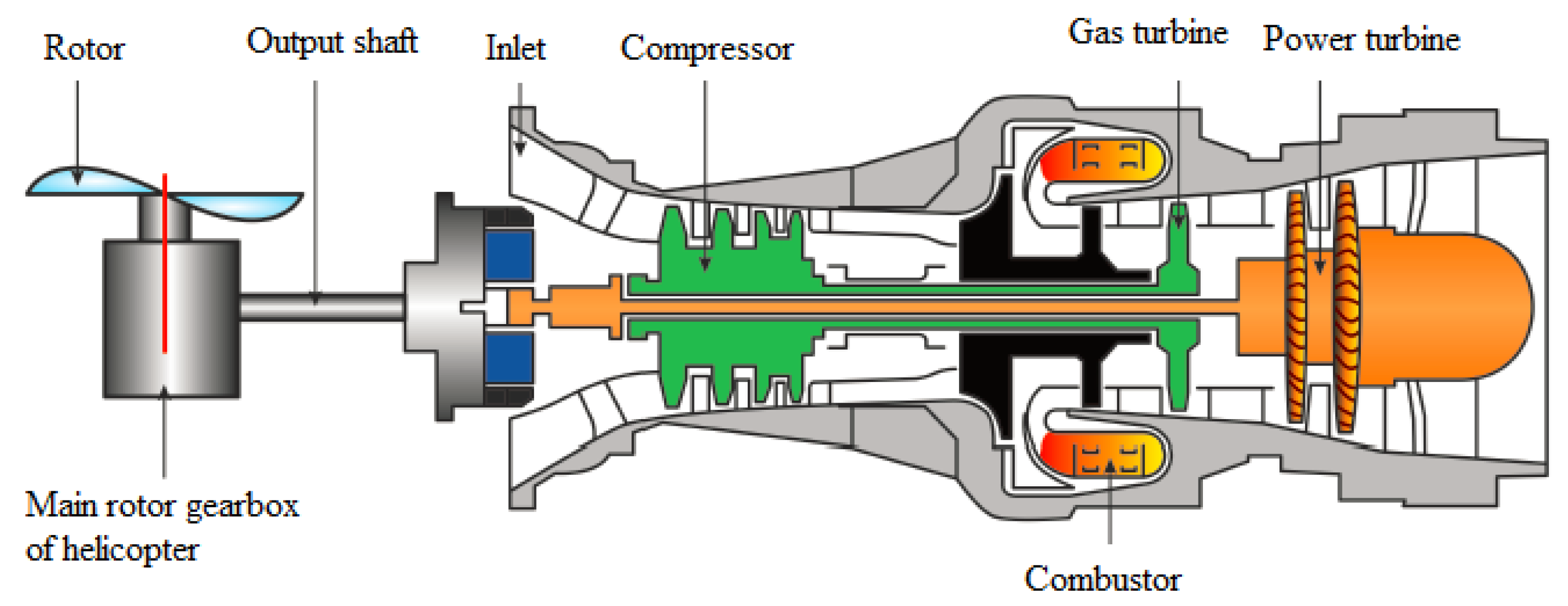
2.1. Brief Introduction of Turbo-Shaft Engine

The sketch of the bi-rotor turbo-shaft engine researched in this paper is shown in Figure 1 [42]. During the operation, the compressed air is drawn from the inlet and flows through the compressor to the combustor where fuel is introduced, mixed, and ignited. Then, the hot gas flows through the gas turbine which extracts a portion of the energy to drive the compressor. Finally, the gas exiting the gas turbine flows through the power turbine which extracts the remaining energy to drive the main rotor [43,44]. All the components work cooperatively to provide power to the helicopter.
For smooth and reliable operation of the helicopter, the rotor speed of the power turbine was always kept at 100% to maintain the main rotor speed constant [42]. This was achieved by adjusting the fuel flow input to the engine. When a flight condition of the helicopter changed, such as forward speed, the required power of the main rotor of the helicopter varied accordingly. This meant that the power turbine needed to provide more or less power to meet the requirement of the main rotor and reach a newly balanced state.

2.2. LPV Model Description

The general discrete state-space equation of LPV model can be described as:
x ( k + 1 ) = A ( α ) x ( k ) + B ( α ) u ( k ) y ( k ) = C ( α ) x ( k ) + D ( α ) u ( k )
where α is the scheduling parameter, u(k) is the input vector of the LPV model, x(k) is the state variable vector, y(k) is the output vector of the LPV model and A(α), B(α), C(α) and D(α) are time-varying matrices scheduled by α.
For turbo-shaft engine, its main dynamic is derived from the cooperative working of the rotor systems [44], which can be described as:
d n g d t = ( W g η g W c ) / [ n g J g ( 30 π ) 2 ] d n p d t = ( W p η p W r ) / [ n p J p ( 30 π ) 2 ]
where ng is the rotor speed of gas turbine, np is the rotor speed of power turbine, Wc, Wg, Wp, Wr are the power values of the compressor, gas turbine, power turbine and main rotor, respectively, ηg and ηp are the shaft efficiency values of the gas turbine and power turbine, respectively and Jg and Jp are the rotor inertia values of the gas turbine and power turbine, respectively.
Equation (2) is a basic equation for the turbo-shaft engine’s dynamic calculation in its mechanism model (for more detail, refer to [42,43,44]). Thus, in research relevant to the state space model of turbo-shaft engines, ng and np are most frequently selected as the state variables [42,43,44,45,46]. In addition, ng can reflect both the output power and the dynamic property of the engine [47,48]. Therefore, the LPV model of turbo-shaft engine can be described in a quasi-LPV form:
x ( k + 1 ) = ( n g ( k + 1 ) n p ( k + 1 ) ) = A ( n g ( k ) ) ( n g ( k ) n p ( k ) ) + B ( n g ( k ) ) W f ( k ) y ( k ) = ( n g ( k ) n p ( k ) P 3 ( k ) T 44 ( k ) ) = C ( n g ( k ) ) ( n g ( k ) n p ( k ) ) + D ( n g ( k ) ) W f ( k )
where ng is selected as both the state variable and the scheduling parameter of the LPV equation, which has α(k) = ng(k). Additionally, np is the controlled variable and another state variable; thus, we have x(k) = [ng(k) np(k)]. The fuel flow Wf is the main control input u(k) = Wf(k). P3 is the total pressure at the compressor exit and T44 is the total temperature at the power turbine inlet. P3, T44 together with ng, are all limit parameters for turbo-shaft engine security which should be taken into consideration in the control system design process to avoid overspeed, overpressure and overtemperature. Therefore, the output vector of the LPV model was set to y(k) = [y1(k) y2(k) y3(k) y4(k)]T = [ng(k) np(k) P3(k) T44(k)]T.
Note that ng and np were already chosen as the states, so its corresponding entries in C and D had a constant value of 0 and 1. For P3 and T44, corresponding entries in matrix C and D varied with the scheduling parameter [15].
In the proposed method, the LPV model was built based on the online training neural network. However, the order of magnitude of the parameters in Equation (3) differed from each other considerably. Therefore, all the data used in the model should be normalized into the order of magnitude of proximity to enhance the accuracy of the model and avoid data overwhelming. The corresponding normalized LPV model is:
x ¯ ( k + 1 ) = ( n ¯ g ( k + 1 ) n ¯ p ( k + 1 ) ) = A ¯ ( n ¯ g ( k ) ) ( n ¯ g ( k ) n ¯ p ( k ) ) + B ¯ ( n ¯ g ( k ) ) W ¯ f ( k ) y ¯ ( k ) = ( n ¯ g ( k ) n ¯ p ( k ) P ¯ 3 ( k ) T ¯ 44 ( k ) ) = C ¯ ( n ¯ g ( k ) ) ( n ¯ g ( k ) n ¯ p ( k ) ) + D ¯ ( n ¯ g ( k ) ) W ¯ f ( k )
where the bar over the variable means that the variable is a normalized parameter, the A ¯ , B ¯ , C ¯ , D ¯ are normalized system and output matrices.
The normalization was carried out as follows:
d ¯ = 2 d d max d min d max d min
where dmax and dmin are the maximum and minimum values of any given variable d.

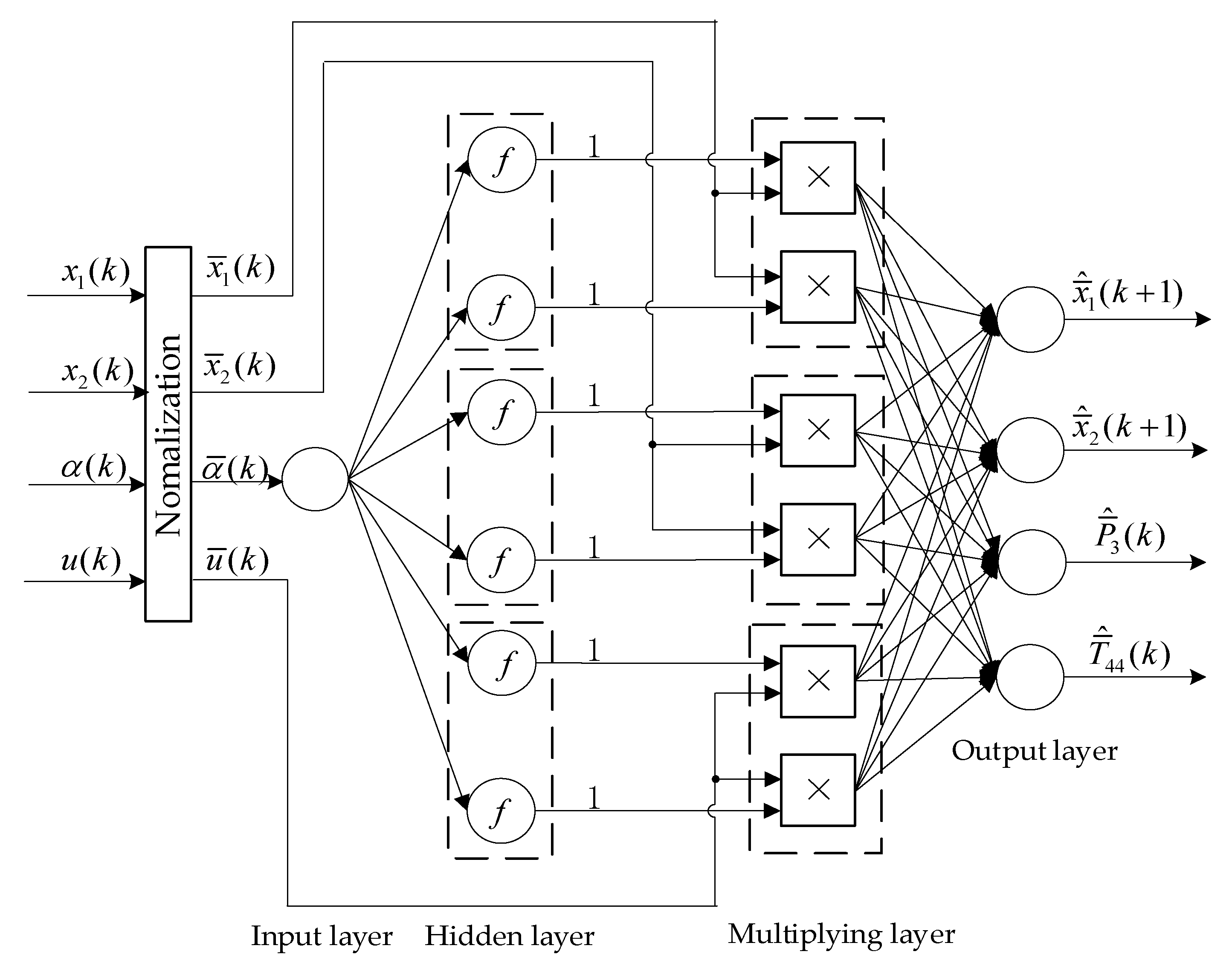
3. Special Structure of MLOS-ELM for DD-LPV Modeling

The online sequential extreme learning machine (OS-ELM) is a kind of single-hidden-layer feedforward neural network (SLFN). It was adopted to train neural networks due to its faster online learning and universal approximation capabilities. In OS-ELM, the training sets of input vector and target vector come one by one or chunk by chunk. For one training data set { ( x i n , t ) } , the OS-ELM model with L additive hidden nodes and activation function f (·) can be formulated as:
y ^ = i = 1 L β i f ( W i x i n + b i )
where y ^ is OS-ELM model’s output, W i is the weight from the input layer to the ith hidden node, bi is the bias of the ith hidden node, βi is the weight from the ith hidden node to the output layer.
For DD-LPV modeling, a special layer called multiplying layer was inserted between the hidden layer and the output layer based on common OS-ELM, as shown in Figure 2. The inputs of the multiplying layer were the outputs of the hidden layer, the normalized states, and the normalized inputs of the LPV model. The output of the multiplying layer node was the product of its inputs.
There were one-to-one local connections between the hidden layer and the multiplying layer, whose weight was set to 1. The nodes of the hidden layer were divided into 3 groups according to the total dimension of x (2-dimension) and u (1-dimension), and each group had 2 nodes, determined by heuristics. Therefore, the outputs of the MLOS-ELM become:
y ^ m = j = 1 2 β j m ( k ) f ( W 1 j α ¯ ( k ) + b j ) x ¯ 1 ( k ) + j = 3 4 β j m ( k ) f ( W 1 j α ¯ ( k ) + b j ) x ¯ 2 ( k ) + j = 5 6 β j m ( k ) f ( W 1 j α ¯ ( k ) + b j ) u ¯ ( k ) m = 1 , 2 , 3 , 4
where y ^ = [ x ¯ ^ 1 ( k + 1 )   x ¯ ^ 2 ( k + 1 )   P ¯ ^ 3 ( k )   T ¯ ^ 44 ( k ) ] T , W 1 j is the weight from the input node to the jth hidden node, bj is the bias of the jth hidden node, β j m is the weight from the jth multiplying layer node to the mth output node. ( β j m is related to time k because it is updated online, while W 1 j and bj are invariant, as detailed in Section 4).
The normalized LPV model of a turbo-shaft engine described by Equation (4), can be written in the form of matrix entries as:
x ¯ ( k + 1 ) = [ x ¯ 1 ( k + 1 ) x ¯ 2 ( k + 1 ) ] = [ a ¯ 11 ( α ¯ ) a ¯ 12 ( α ¯ ) a ¯ 21 ( α ¯ ) a ¯ 22 ( α ¯ ) ] [ x ¯ 1 ( k ) x ¯ 2 ( k ) ] + [ b ¯ 1 ( α ¯ ) b ¯ 2 ( α ¯ ) ] u ¯ ( k ) y ¯ ( k ) = [ x ¯ 1 ( k ) x ¯ 2 ( k ) P ¯ 3 ( k ) T ¯ 44 ( k ) ] = [ 1 0 0 1 c ¯ 31 ( α ¯ ) c ¯ 32 ( α ¯ ) c ¯ 41 ( α ¯ ) c ¯ 42 ( α ¯ ) ] [ x ¯ 1 ( k ) x ¯ 2 ( k ) ] + [ 0 0 d ¯ 3 ( α ¯ ) d ¯ 4 ( α ¯ ) ] u ¯ ( k )
According to Equation (7), the entries of A ¯ ( α ¯ ) , B ¯ ( α ¯ ) , C ¯ ( α ¯ ) , D ¯ ( α ¯ ) in Equation (8) were obtained:
A ¯ ( α ¯ ) = [ j = 1 2 β j 1 ( k ) f ( W 1 j α ¯ ( k ) + b j ) j = 3 4 β j 1 ( k ) f ( W 1 j α ¯ ( k ) + b j ) j = 1 2 β j 2 ( k ) f ( W 1 j α ¯ ( k ) + b j ) j = 3 4 β j 2 ( k ) f ( W 1 j α ¯ ( k ) + b j ) ] B ¯ ( α ¯ ) = [ j = 5 6 β j 1 ( k ) f ( W 1 j α ¯ ( k ) + b j ) j = 5 6 β j 2 ( k ) f ( W 1 j α ¯ ( k ) + b j ) ] T C ¯ ( α ¯ ) = [ 1 0 0 1 j = 1 2 β j 3 ( k ) f ( W 1 j α ¯ ( k ) + b j ) j = 3 4 β j 3 ( k ) f ( W 1 j α ¯ ( k ) + b j ) j = 1 2 β j 4 ( k ) f ( W 1 j α ¯ ( k ) + b j ) j = 3 4 β j 4 ( k ) f ( W 1 j α ¯ ( k ) + b j ) ] D ¯ ( α ¯ ) = [ 0 0 j = 5 6 β j 3 ( k ) f ( W 1 j α ¯ ( k ) + b j ) j = 5 6 β j 4 ( k ) f ( W 1 j α ¯ ( k ) + b j ) ] T
As can be seen from Equation (9), the non-constant elements of A ¯ , B ¯ , C ¯ , D ¯ in Equation (4) were derived from the parameters of the MLOS-ELM, varying with the scheduling parameter α and output weight β. By inserting a multiplying layer between the hidden layer and the output layer, the output function of the MLOS-ELM was presented in the mathematical description form of the LPV model. That meant that the weights and the input scheduling parameter of the MSOL-ELM were given the ability to derive the parameters of the LPV model. In other words, Equation (9) linked the neural network model and the LPV model closely, which made the LPV model able to be derived directly and conveniently by the network’s inner parameters at every sample time k.
Remark 1.
The numbers of the hidden nodes and the multiplying nodes were both set to 6 by heuristics in this research, which was sufficient to achieve an accurate MLOS-ELM model. The smallest number of nodes in each group was 2, to ensure the accuracy of the MLOS-ELM in this research. If each group had only 1 node, MLOS-ELM’s accuracy would have been negatively affected. However, if each group had more than 2 nodes, its accuracy would not be improved but the computational burden would increase rapidly. Moreover, they could be set to different numbers (no less than 3) separately. Owing to there being 3 independent state and input variables x ¯ 1 , x ¯ 2 , u ¯ in turbo-shaft engine’s LPV model, the nodes in the multiplying layer must be divided into 3 groups, evenly or not. Then, the output of the network would always have the expression in form of Equation (7) which in turn had an LPV form. The even structure presented in the paper was simple and easily described.
Remark 2.
MLOS-ELM’s input layer had only one input (the 1-dimensional scheduling parameter α ¯ ( k ) = n ¯ g ( k ) ) which was enough to express the variation of the matrices of the DD-LPV model. Other factors that could have affected the matrices, such as Mach number Ma or altitude H, were not used as the inputs because the online training method was adopted. Therein, the output weight of the network was adapted to the current working condition, including the Mach number and the altitude change, so the entries in Equation (9) could automatically adjust according to the flying condition. Moreover, taking more parameters as the inputs of MLOS-ELM could have affected the accuracy of the DD-LPV.

4. Online Updating Algorithm of MLOS-ELM

OS-ELM was utilized to build the network for its high real-time properties and competence in recursive learning. The convergence of OS-ELM was proven in [49]. At each sample time k, the newly gathered data set was used to update OS-ELM’s output weight β.
According to the MLOS-ELM described in Figure 2. the output vector of the hidden layer at sample time k is:
H ( k ) = [ h 1 ( k ) h 2 ( k ) h 6 ( k ) ]     = [ f ( W 11 α ¯ ( k ) + b 1 )   f ( W 12 α ¯ ( k ) + b 2 )     f ( W 16 α ¯ ( k ) + b 6 ) ]
where W R 1 × 6 and b R 1 × 6 are randomly generated at the first time step and kept constant, f ( W α ¯ + b ) = 1 1 + e ( W α ¯ + b ) .
Then the output vector of the multiplying layer is:
O ( k ) = [ h 1 ( k ) x ¯ 1 ( k )   h 2 ( k ) x ¯ 1 ( k )   h 3 ( k ) x ¯ 2 ( k )   h 4 ( k ) x ¯ 2 ( k )   h 5 ( k ) u ¯ ( k )   h 6 ( k ) u ¯ ( k ) ]
The outputs of MLOS-ELM model of Equation (7) can be rewritten in a compact form:
y ^ ( k ) = O ( k ) β ( k ) t ( k )
where β R 6 × 4 , t ( k ) = [ x ¯ 1 ( k + 1 )   x ¯ 2 ( k + 1 )   P ¯ 3 ( k )   T ¯ 44 ( k ) ] T is the target vector.
If k = 1, the weight β can be calculated by least square method:
β ( 1 ) = ( O T ( 1 ) O ( 1 ) ) 1 O T ( 1 ) t ( 1 )
However, O ( 1 ) R 1 × 6 has rank 1 (not full column rank), thus O ( 1 ) T O ( 1 ) is singular. Then the ridge regression theory is used to rewrite Equation (13):
β ( 1 ) = ( O ( 1 ) T O ( 1 ) + λ I ) 1 O ( 1 ) T t ( 1 )
where λ is the generalized regularization parameter.
If k > 1, the output weight β was updated recursively online every sampling period to adapt to the new working state of the engine. However, in some instances, the outputs of MLOS-ELM already matched the target outputs well with previous output weight, especially at a steady state. Under such conditions, there was no need to update the output weight at every sampling time, which increased the computational burden. Therefore, a criterion was set to judge whether the output weight needed to be updated according to the output error of the network.
The output error was defined by relative percentage error:
e r r i ( k ) = y ^ i ( k ) t i ( k ) t i ( k ) × 100 %
If one of MLOS-ELM’s output errors erri, i = 1,2,3,4 exceeded the update criterion, the recursive least square method was used to update the weight according to the new gathered data. Otherwise, the weight maintained the same value as the last sampling time.
Then we have the output weight β(k) (k > 1) as:
If | e r r i ( k ) | < δ i ,   i = 1 , 2 , 3 , 4
β ( k ) = β ( k 1 )
else
{ β ( k ) = β ( k 1 ) + P ( k ) O T ( k ) ( t ( k ) y ^ ( k ) ) P ( k ) = P ( k 1 ) P ( k 1 ) O ( k ) O T ( k ) P ( k 1 ) 1 + O T ( k ) P ( k 1 ) O ( k )
where δ i > 0 ,   i = 1 , 2 , 3 , 4 is the maximum allowable output error of MLOS-ELM, P ( 1 ) is defined as P ( 1 ) = ( O T ( 1 ) O ( 1 ) + λ I ) 1 .
Combining Section 3 and Section 4, the proposed online DD-LPV modeling method of turbo-shaft engine based on MLOS-ELM can be summarized in the following steps:
  • Step 1. Randomly generate the hidden layer parameters W and b, set δ and λ ;
  • Step 2. Update the output weight β ( k ) : If k = 1, Equation (14) is used. Otherwise, Equation (16) or Equation (17) is used;
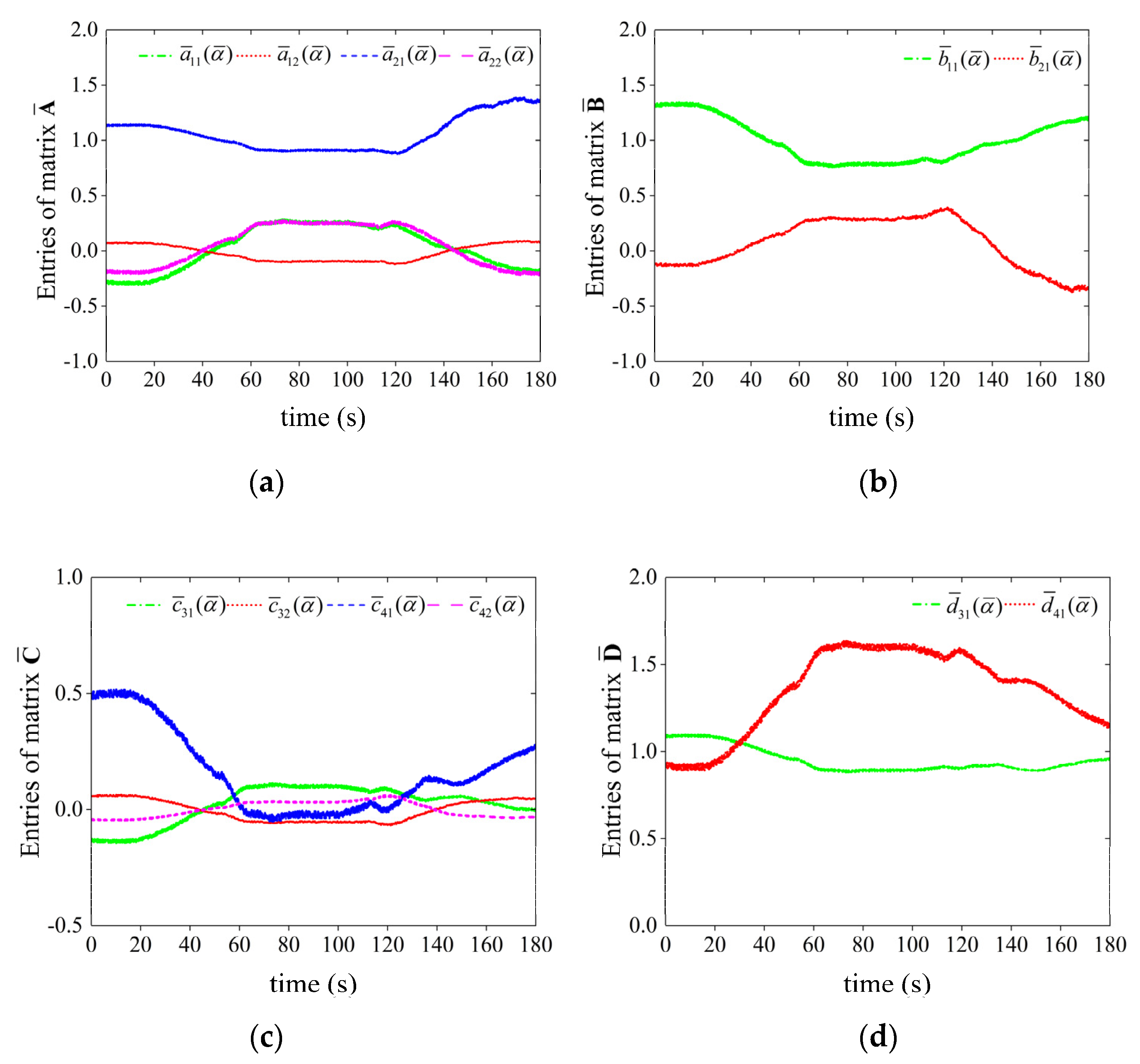
  • Step 3. Calculate the LPV system matrices A ¯ ( α ¯ ) , B ¯ ( α ¯ ) , C ¯ ( α ¯ ) , D ¯ ( α ¯ ) according to Equation (9);
  • Step 4. Set k = k + 1, go back to Step 2.
Remark 3.
To be consistent with the description of the discrete state space equation in Equation (4), the outputs of MLOS-ELM and the target vector in Equation (12) included states at time k + 1. Since the data at time k + 1 could not be collected online at time k in real applications, the DD-LPV model at time k was obtained by the data of the states at time k and the outputs at time k − 1.

5. Simulation and Discussions

To verify the accuracy of the MLOS-ELM network and the online DD-LPV model derived from it, simulations in the flight envelope were carried out based on the component level model (CLM) of the UH-60 helicopter and T700 engine system platform for lack of rig test data. The accuracy of this integrated UH-60 helicopter and T700 engine model was checked and verified in [44,50] by a great number of tests. The test results prove that the integrated model not only had good reliability, but was able to carry out digital flight simulations of routine missions [44]. The data generated by the integrated model had high fidelity. For more detailed information, refer to [43,44,51].
The output weight update criteria of MLOS-ELM were δ i = 0.005 ,   i = 1 , 2 , 3 , 4 and λ = 10 8 . The anti-normalized outputs were adopted to evaluate the accuracy of the MLOS-ELM and the DD-LPV model with physical value.
The true value of the outputs was attained by anti-normalization according to Equation (5):
d = d ¯ ( d max d min ) + d max + d min 2
In Section 5.1 and Section 5.2, all comparisons and relative errors were calculated by anti-normalized data.

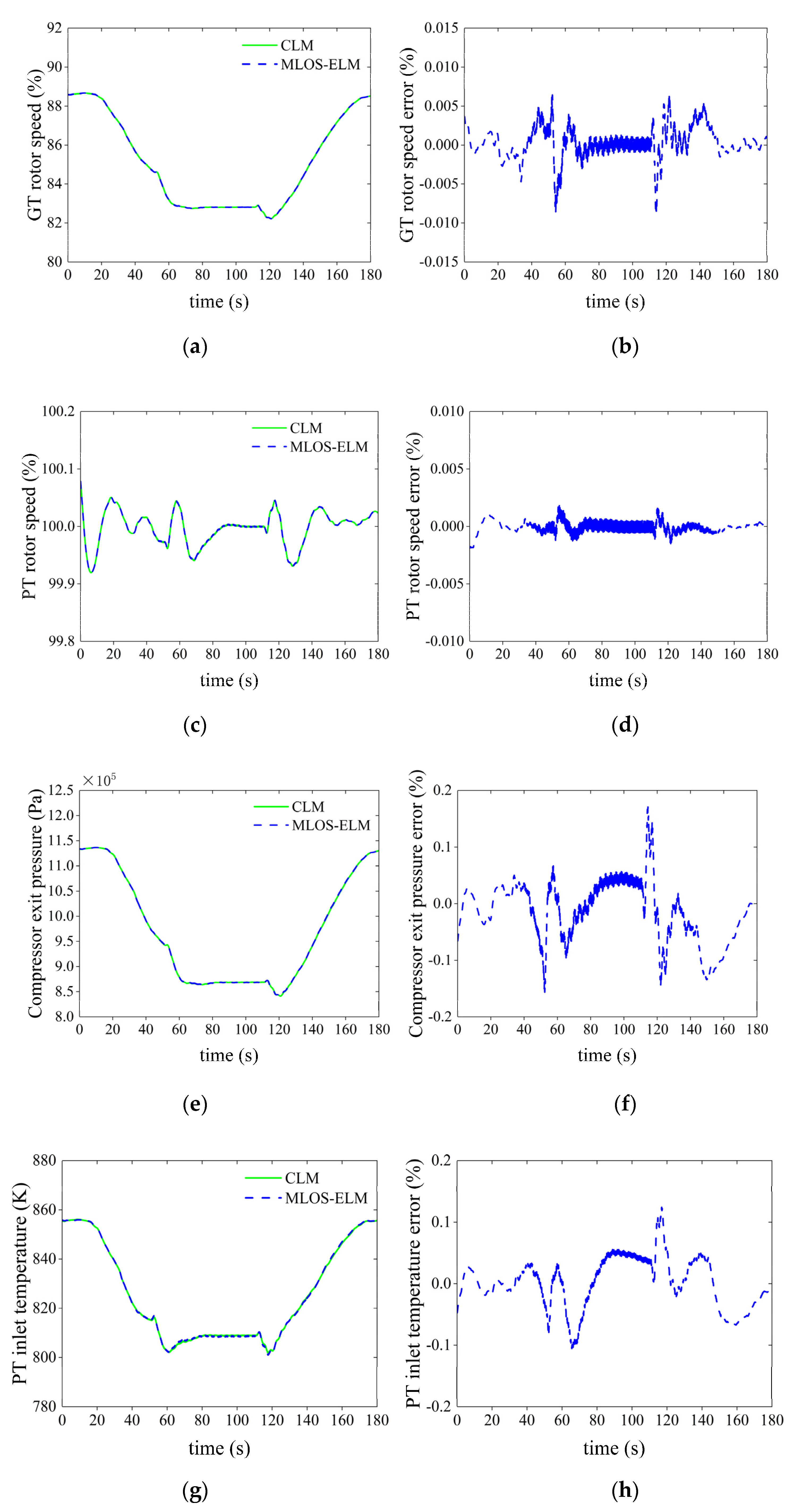
5.1. Approximation Ability Verification of the MLOS-ELM

First, the effectiveness of the proposed MLOS-ELM was tested through simulation. The target values of t were gathered online from the component level model (CLM) of the turbo-shaft engine. The purpose of this section was to validate whether the output of MLOS-ELM y ^ could track the output of CLM accurately.
The simulation was first carried out at altitude 0 m, with the trajectory of the forward speed of the helicopter increasing from 0 m/s to 30 m/s in the first 50 s, remaining invariant for 60 s and then decreasing to 0 m/s in the last 70 s, as shown in Figure 3. The turbo-shaft engine was controlled to keep the power turbine rotor speed at 100% during the whole process.
The comparisons of the MLOS-ELM network’s output and the CLM’s output are shown in Figure 4. In the figure, GT represents the gas turbine and PT represents the power turbine.
It can be seen from Figure 4 that the rotor speed response of the MLOS-ELM was able to match that of the CLM accurately during both the steady state and the dynamic process. The relative error of MLOS-ELM outputs to those of CLM was less than 0.009% for GT rotor speed and 0.003% for PT rotor speed. The error of compressor exit pressure and PT inlet temperature was also very small, which was within 0.18% and 0.12%, respectively. When the helicopter switched from acceleration to constant speed at 50 s and from constant speed to deceleration at 110 s, the network could still track the outputs well (though a sudden change of the forward speed trajectory occurred). The simulation results showed that the special OS-ELM, with an additional multiplying layer, achieved a high degree of approximation accuracy, which implied the effectiveness of the online DD-LPV model derived by MLOS-ELM.

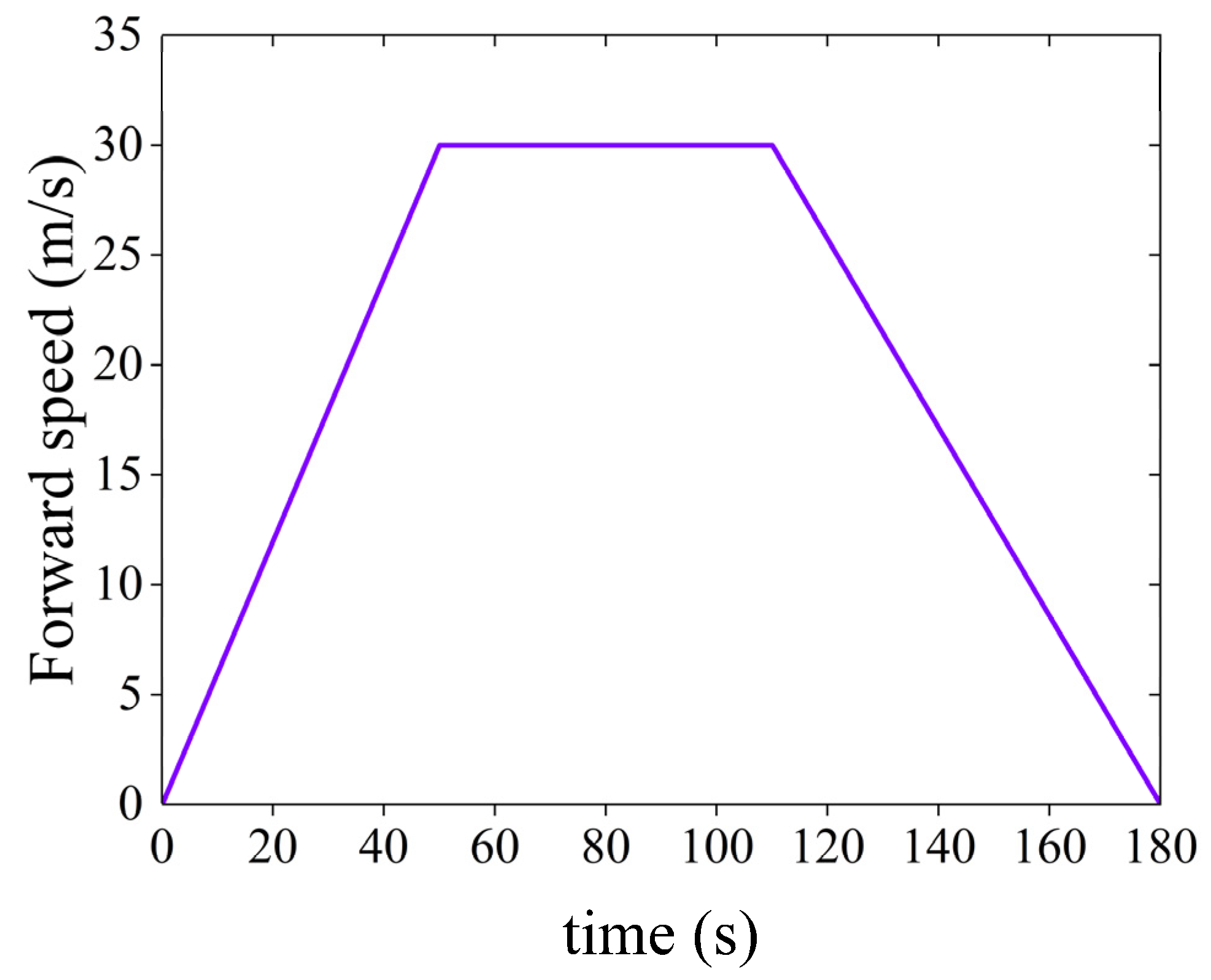
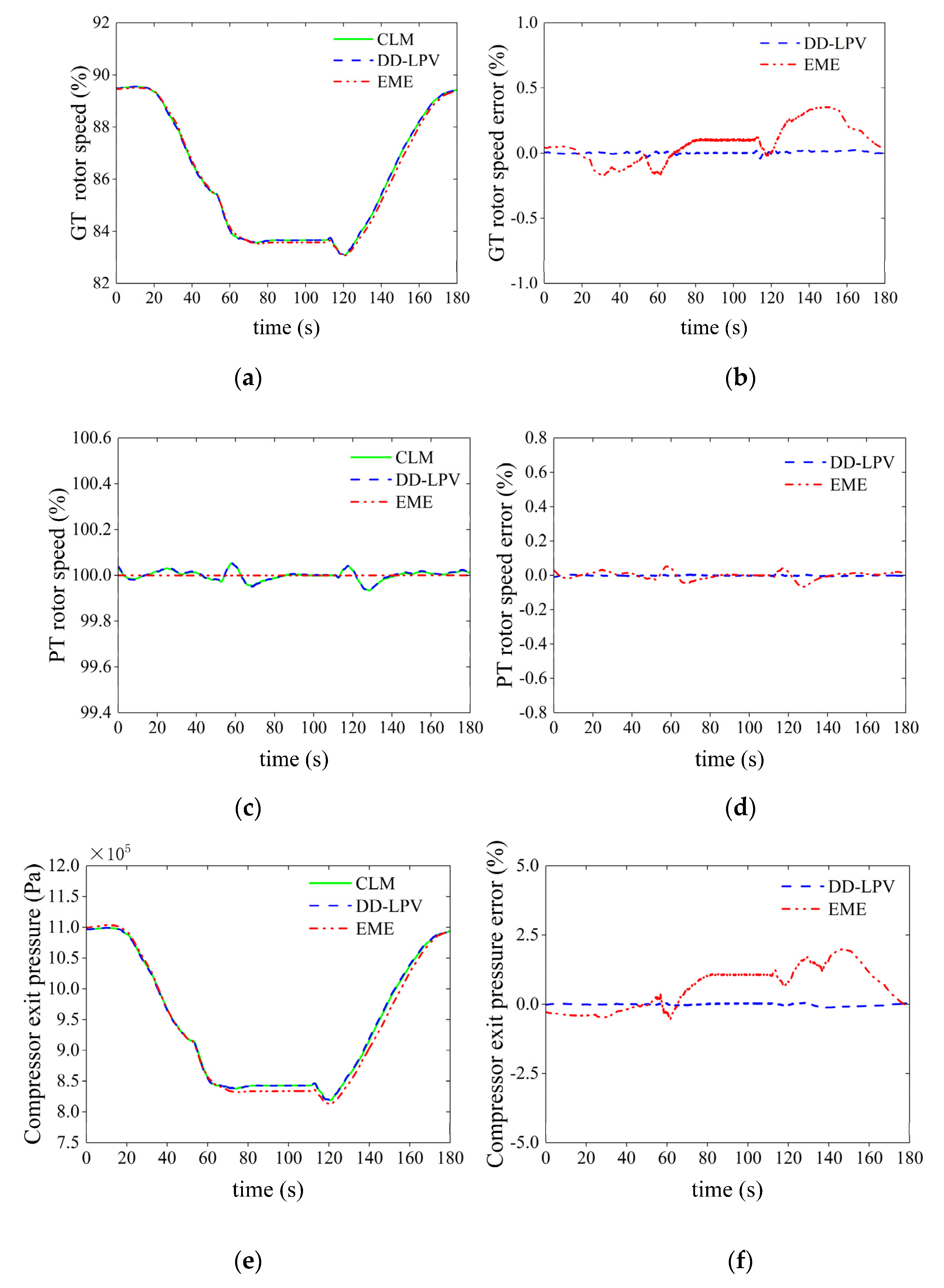
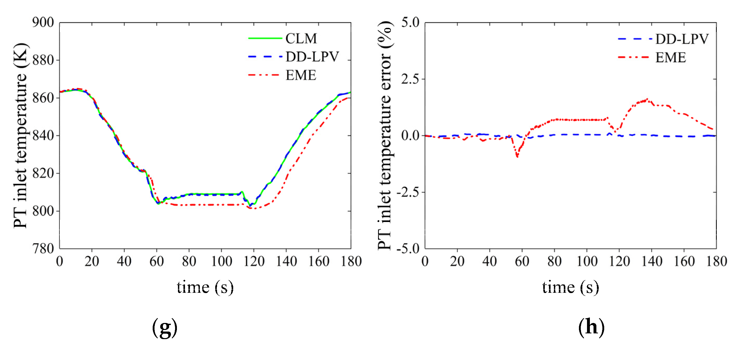
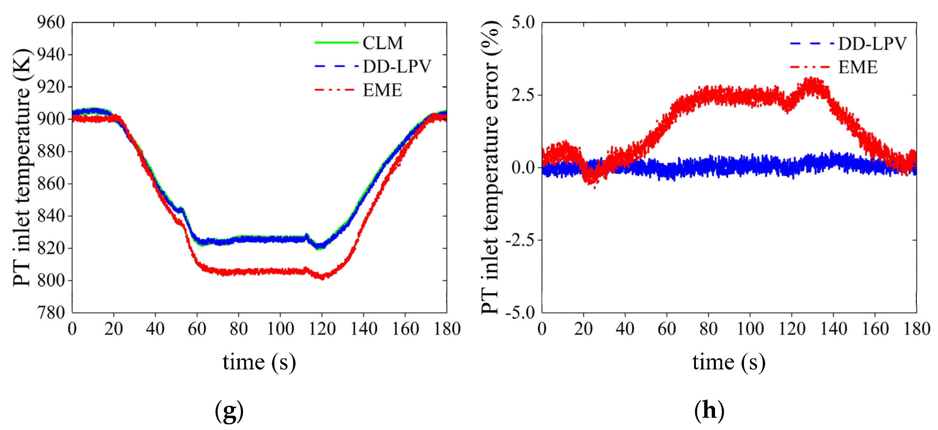
5.2. Prediction Ability Validation of the Online DD-LPV Model in Flight Envelope

The online DD-LPV model was designed to be used in MPC or PSC, whose model was to predict the future outputs of the next few sample times. Therefore, in this section, the prediction ability of the proposed DD-LPV model was validated.
For the LPV model derived from the MLOS-ELM at time k, its state space equation matrices were A ¯ ( k ) , B ¯ ( k ) , C ¯ ( k ) , D ¯ ( k ) . Its prediction outputs at time k + p were obtained with the input series of the CLM over time k to k + p, and compared with the CLM output at time k + p to verify the prediction ability of the LPV model derived at time k. As k moved along the test horizon, the prediction ability of the models derived at each sampling time were tested.
The prediction outputs of the LPV model were acquired by the response calculation of the discrete time system:
x ¯ ( k + 1 ) = A ¯ ( k ) x ¯ CLM ( k ) + B ¯ ( k ) u ¯ CLM ( k ) x ¯ ( k + 2 ) = A ¯ ( k ) x ¯ ( k + 1 ) + B ¯ ( k ) u ¯ CLM ( k + 1 )   = A ¯ 2 ( k ) x ¯ CLM ( k ) + A ¯ ( k ) B ¯ ( k ) u ¯ CLM ( k ) + B ¯ ( k ) u ¯ CLM ( k + 1 )
Proceeding forward from Equation (19), we can obtain x ¯ ( k + p ) and then y ¯ ( k + p ) :
x ¯ ( k + p ) = A ¯ p ( k ) x ¯ CLM ( k ) + m = k k + p 1 A ¯ k + p 1 m ( k ) B ¯ ( k ) u CLM ( m ) y ¯ ( k + p ) = C ¯ ( k ) A ¯ p ( k ) x ¯ CLM ( k ) + m = k k + p 1 C ¯ ( k ) A ¯ k + p 1 m ( k ) B ¯ ( k ) u CLM ( m ) + D ¯ ( k ) u CLM ( k + p )
As a recently proposed data-driven modeling method for aero engines, an equilibrium manifolds expansion (EME) model [35,36,37] was also built on the UH-60/T700 system for prediction ability comparison. The EME model for the turbo-shaft engine was built at an altitude of 1000 m with different power requirements of the helicopter and was extended to the entire flight envelope through similarity transformation [37].
The simulations were carried out at altitudes of 1000 m and 3000 m with the same forward speed variation in Figure 3. The prediction results of k + 5 at 1000 m are shown in Figure 5 and the variations of the DD-LPV model parameters during this process are shown in Figure 6. Figure 7 shows the prediction results of k + 5 at 3000 m and the variation of the corresponding DD-LPV model parameters are shown in Figure 8. Random noises (magnitude 0.2%) were added to the data gathered from the CLM at 3000 m to imitate the measurement noise, which meant that the MLOS-ELM model at 3000 m was trained by the data with noise—and so was the DD-LPV model derived from it.
Figure 5 shows that future output prediction at time k + 5 of the online DD-LPV model was able to match that of the CLM more accurately than the EME model when the altitude was set to 1000 m. The relative predictive errors at time k + 5 of DD-LPV model rotor speed to that of CLM were less than 0.05% for GT rotor speed and less than 0.01% for PT rotor speed. The maximum errors of compressor exit pressure and PT inlet temperature were less than 0.13% and 0.12% respectively, which meant that the DD-LPV model achieved high accuracy in the prediction of all output parameters. At 50 s and 110 s, when the forward speed switched, the fluctuation ranges of the prediction error were also very small. Meanwhile, as shown in Figure 5, the EME model’s relative predictive errors of these four outputs were less than 0.36%, 0.07%, 2.0% and 1.7%, respectively. Although the accuracy of the EME model, whose similarity transformation was computed at the similar inlet pressure and temperature, was still acceptable at 1000 m, its prediction error was still much greater than that of the online identified DD-LPV model.
Figure 6 shows that some of the parameters, such as a ¯ 12 ( α ¯ ) , a ¯ 21 ( α ¯ ) and b ¯ 21 ( α ¯ ) , changed very slightly, even their corresponding scheduling parameter α ¯ ( k ) = n ¯ g ( k ) changed within a relatively wide range. Thus, the output weight β(k) of the MLOS-ELM changed accordingly because the parameters of the DD-LPV model were changed not only with the scheduling parameter, but also with the online updated output weight. All the parameters of the LPV model varied smoothly during the forward speed increase and decrease process which guaranteed the DD-LPV model the ability of smooth prediction over the test horizon. ( c ¯ 11 ( α ¯ ) ~ c ¯ 22 ( α ¯ ) , d ¯ 11 ( α ¯ ) ~ d ¯ 21 ( α ¯ ) are not shown in the figure since they were fixed values of 1 or 0).
It can be seen from Figure 7 that all the future outputs prediction of the online DD-LPV model was able to track that of the CLM at time k + 5 very well with measurement noise considered. Most of the relative errors fluctuated around the magnitude of 0.2% which was consistent with the magnitude of the measurement noise. The rotor speed prediction error of the LPV model at time instant k + 5 was less than 0.35%. Most compressor exit pressure prediction errors of the online DD-LPV model at time instant k + 5 were less than 0.6%, and the maximum error was less than 0.81%. All the GT inlet temperature prediction errors were less than 0.6%. By contrast, the maximum prediction errors of P3 and T44 of the EME model increased greatly, up to 2.62% and 3.17%, respectively, when the flying altitude changed to 3000 m.
Figure 8 shows that the parameters of the DD-LPV model varied in a wider range than that at altitude 1000 m with the same forward speed variation and a much similar scheduling parameter variation range. If the measurement noise was not considered, similar parameter variations resulted, as Figure 6 illustrates. This meant that the changes were aroused by the measurement noise added to the online training data of the MLOS-ELM, which in turn affected the parameters of the DD-LPV model. Even so, all the parameters of the DD-LPV model still changed smoothly during the dynamic process.
To further verify the effectiveness of the proposed online DD-LPV model, online prediction comparations of the DD-LPV model and the EME model (at different altitudes with and without measurement noise) were conducted. The results are listed in Table 1.
It can be seen from Table 1 that the online DD-LPV model was able to predict future outputs more accurately than the EME model at different altitudes within the flight envelope.
Without measurement noise considered, the average prediction errors of Ng of the DD-LPV model were between 0.0071% and 0.0115%—much smaller than those of the EME model, which were between 0.1258% and 0.2134%. For Np, the range of the average errors of DD-LPV model was between 0.0011% and 0.0025%, and was also smaller than that of EME model which was between 0.0150% and 0.0222%. For P3 and T44, much better prediction results could be achieved by the online DD-LPV model. For P3, the average errors of DD-LPV model were between 0.0172% and 0.0896% while those of EME model were between 0.6233% and 1.1080%. For T44, the average errors of DD-LPV model were between 0.0165% and 0.0471% while those of EME model were between 0.5714% and 1.4431%. Additionally, the maximum errors of Ng, Np, P3 and T44 of DD-LPV model were also obviously better than the EME model. Moreover, the performance of output prediction of the DD-LPV model was more stable, with the most standard deviation lower by more than an order of magnitude, compared with the EME model. Furthermore, the DD-LPV model had no obvious prediction error fluctuations when the altitude and the forward flying speed changed. It identified those changes instantly, according to the online gathered data. On the contrary, from 1000 m to 4000 m, the EME model’s average prediction errors of P3 and T44 showed a clearly increasing trend from 0.7899% and 0.5714% to 1.1080% and 1.4431%, respectively, mainly contributing to the turbo-shaft engine’s poor applicability of similarity transformation.
With measurement noise considered, the average prediction errors of the online DD-LPV model’s four outputs Ng, Np, P3 and T44 were within 0.1202%, 0.1125%, 0.2320%, and 0.1895%, respectively, and the maximum errors were less than 0.4447%, 0.3825%, 1.0303% and 0.8425%, obviously better than the EME model. However, it was notable that the average prediction errors of the EME model were not greatly changed with or without the measurement noise, while, for the DD-LPV model, the prediction errors increased greatly with noise considered. This was mainly because the original error of the DD-LPV model without noise considered was much smaller than the magnitude of the noise. As an online training method, noise will affect the update of the output weight, which in turn will affect the accuracy of MLOS-ELM and the DD-LPV model derived from it.

6. Conclusions

This paper proposed an online data-driven LPV modeling method for turbo-shaft engines using the online sequential extreme learning machine with an additional multiplying layer (MLOS-ELM). Through simulations conducted in a wide fight envelope, several conclusions were drawn.
First, the outputs of the proposed MLOS-ELM were able to track the outputs of the CLM online precisely, which demonstrated that the MLOS-ELM was able to model the turbo-shaft engine dynamic accurately. The insertion of the multiplying layer made the output of the network become a state space LPV form without affecting the approximation accuracy. Hence, the MLOS-ELM could represent a new thought for data-driven modeling methods that deserves further research. It has the potential to adapt to the properties of other individual engine or nonlinear systems.
When the traditional state space modeling methods of for aero engines were carried out based on applying small perturbations on the CLM, the DD-LPV modeling method based on MLOS-ELM provided a CLM-free online linear model identification method. It was able to avoid the modeling errors of the CLM and enhance the accuracy of the LPV model, especially at the dynamic state.
The DD-LPV modeling method was very efficient and convenient. It was able to derive an accurate LTI state space model instantly at each sampling time with the individual engine online gathered data, which made the LPV model free from the influence of engine degradation and usable as an adaptive LPV model. Additionally, it could lower the mechanism modeling burden of physical systems for linearization purposes.
Differing from the EME model, which needed the similarity transformation to be applied to the whole flying envelope, the proposed DD-LPV model was derived online, and was able to match variations in flying conditions well. Future output prediction simulation results showed that the online DD-LPV model could be used to predict the output of the aero engine over the next several steps much more precisely than the EME model, with or without the measurement noise considered.
Therefore, the proposed modeling method based on MLOS-ELM represents a new and promising data-driven online modeling method that is worthy of further research in control system designs where LPV models are widely used, such as MPC, fault diagnosis, performance seeking control, and so on.

Author Contributions

Conceptualization, Q.L.; methodology, Z.G. and S.P.; software, Z.G.; validation, Z.G., S.P. and Y.L.; formal analysis, Z.G.; investigation, Z.G.; resources, Z.G. and Y.L.; data curation, Z.G. and Q.L.; writing—original draft preparation, Z.G.; writing—review and editing, Z.G., S.P. and Q.L.; visualization, Z.G.; supervision, Q.L.; project administration, W.Z.; funding acquisition, W.Z. All authors have read and agreed to the published version of the manuscript.

Funding

This study was supported by the National Science and Technology Major Project (J2019-I-0010-0010).

Institutional Review Board Statement

Not applicable.

Informed Consent Statement

Not applicable.

Data Availability Statement

Data sharing is not applicable to this article.

Conflicts of Interest

The authors declare no conflict of interest.

References

  1. Lacerda, M.J.; Palhares, R.M. On discrete-time LPV control using delayed Lyapunov functions. Asian J. Control 2021, 23, 2359–2369. [Google Scholar]
  2. Lao-atiman, W.; Olaru, S.; Diop, S.; Skogestad, S.; Arpornwichanop, A.; Cheacharoen, R.; Kheawhom, S. Linear parameter-varying model for a refuellable zinc–air battery. R. Soc. Open Sci. 2020, 7, 201107. [Google Scholar] [CrossRef] [PubMed]
  3. Zhao, M.; Jiang, C.C.; Tang, X.M.; She, M.H. Interpolation Model Predictive Control of Nonlinear Systems Described by Quasi-LPV Model. Autom. Control Comput. Sci. 2018, 52, 354–364. [Google Scholar] [CrossRef]
  4. Liu, X.; Han, G.; Yang, X. Robust Global Identification of LPV Errors-in-Variables Systems with Incomplete Observations. IEEE Trans. Syst. Man Cybern. Syst. 2021, 1–9. [Google Scholar] [CrossRef]
  5. Yue, X.; Su, B. Predictive Functional Control of Nonlinear Systems Based on Multiple LPV Models. In Proceedings of the 2019 Chinese Automation Congress, Hangzhou, China, 1 November 2019. [Google Scholar]
  6. Atam, E. Advanced Air Path Control in Diesel Engines Accounting for Variable Operational Conditions. IEEE Access 2018, 6, 42165–42176. [Google Scholar] [CrossRef]
  7. Samadzadeh, S.; Mazinan, A.H. LMI-based LPV control strategy considering UAV systems. Spat. Inf. Res. 2019, 27, 425–431. [Google Scholar] [CrossRef]
  8. Hang, P.; Chen, X. Path tracking control of 4-wheel-steering autonomous ground vehicles based on linear parameter-varying system with experimental verification. Proc. Inst. Mech. Engineers. Part I J. Syst. Control. Eng. 2021, 235, 411–423. [Google Scholar] [CrossRef]
  9. Alcalá, E.; Puig, V.; Quevedo, J.; Rosolia, U. Autonomous racing using Linear Parameter Varying-Model Predictive Control (LPV-MPC). Control Eng. Pract. 2020, 95, 104270. [Google Scholar] [CrossRef]
  10. Lim, J.; Kirchen, P.; Nagamune, R. LPV Controller Design for Diesel Engine SCR Aftertreatment Systems Based on Quasi-LPV Models. IEEE Control Syst. Lett. 2020, 5, 1807–1812. [Google Scholar] [CrossRef]
  11. Gidon, D.; Abbas, H.S.; Bonzanini, A.D.; Graves, D.B.; Velni, J.M.; Mesbah, A. Data-driven LPV model predictive control of a cold atmospheric plasma jet for biomaterials processing. Control Eng. Pract. 2021, 109, 104725. [Google Scholar] [CrossRef]
  12. López-Estrada, F.R.; Rotondo, D.; Valencia-Palomo, G. A review of convex approaches for control, observation and safety of linear parameter varying and Takagi-Sugeno systems. Processes 2019, 7, 814. [Google Scholar] [CrossRef] [Green Version]
  13. Hoffmann, C.; Werner, H. A survey of linear parameter-varying control applications validated by experiments or high-fidelity simulations. IEEE Trans. Control Syst. Technol. 2014, 23, 416–433. [Google Scholar] [CrossRef]
  14. Sun, T.; Sun, X.M.; Sun, A. Optimal Output Tracking of Aircraft Engine Systems: A Data-driven Adaptive Performance Seeking Control. IEEE Trans. Circuits Syst. II Express Briefs 2021. [Google Scholar] [CrossRef]
  15. Pang, S.W.; Li, Q.H.; Zhang, H.B. A new online modelling method for aircraft engine state space model. Chin. J. Aeronaut 2020, 33, 1756–1773. [Google Scholar] [CrossRef]
  16. Cox, P.B.; Tóth, R. Linear parameter-varying subspace identification: A unified framework. Automatica 2021, 123, 109296. [Google Scholar] [CrossRef]
  17. Guangdeng, Z.; Yang, D.; Lam, J.; Song, X. Fault-tolerant control of switched LPV systems: A bumpless transfer approach. IEEE/ASME Trans. Mechatron. 2021. [Google Scholar] [CrossRef]
  18. Salt Ducajú, J.M.; Salt Llobregat, J.J.; Cuenca, Á.; Tomizuka, M. Autonomous ground vehicle lane-keeping LPV model-based control: Dual-rate state estimation and comparison of different real-time control strategies. Sensors 2021, 21, 1531. [Google Scholar] [CrossRef]
  19. Rotondo, D.; Nejjari, F.; Puig, V. Quasi-LPV modeling, identification and control of a twin rotor MIMO system. Control Eng. Pract. 2013, 21, 829–846. [Google Scholar] [CrossRef]
  20. Ferranti, F.; Rolai, Y. Modeling of linear parameter-varying systems using interpolation of root macromodels and scaling coefficients. Mech. Syst. Signal Process. 2015, 60, 836–852. [Google Scholar] [CrossRef]
  21. Ferranti, F.; Rolain, Y. A local approach for the modeling of linear parameter-varying systems based on transfer function interpolation with scaling coefficients. In Proceedings of the Instrumentation & Measurement Technology Conference, Pisa, Italy, 11–14 May 2015; IEEE: Manhattan, NY, USA, 2015; pp. 606–611. [Google Scholar]
  22. Marcos, A.; Balas, G.J. Development of Linear-Parameter-Varying Models for Aircraft. J. Guid. Control Dyn. 2004, 27, 218–228. [Google Scholar] [CrossRef] [Green Version]
  23. De Caigny, J.; Camino, J.F.; Swevers, J. Interpolating model identification for SISO linear parameter-varying systems. Mech. Syst. Signal Process. 2009, 23, 2395–2417. [Google Scholar] [CrossRef]
  24. Chen, Q.J.; Huang, J.Q.; Pan, M.X.; Lu, F. A Novel Real-Time Mechanism Modeling Approach for Turbofan Engine. Energies 2019, 12, 3791. [Google Scholar] [CrossRef] [Green Version]
  25. Sun, H.B. Design of Linear Parameter Varying Controllers for Turbo-Fan Engines; Nanjing University of Aeronautics and Astronautics: Nanjing, China, 2018. (In Chinese) [Google Scholar]
  26. Liu, J.F.; Ma, Y.J.; Zhu, L.H.; Zhao, H.; Liu, H.P.; Yu, D.R. Improved. Gain Scheduling Control and Its Application to Aero-Engine LPV Synthesis. Energies 2020, 3, 5976. [Google Scholar] [CrossRef]
  27. Sun, H.B.; Pan, M.X.; Huang, J.Q. Switching control for turbofan engine based on Double-Layer LPV Model. J. Propuls. Technol. 2018, 39, 2828–2838. [Google Scholar]
  28. Lv, C.K.; Chang, J.T.; Yu, D.R. Feedback Linearized Sliding Mode Control of Turbofan Engine Based on Multiple Input Multiple Output Equilibrium Manifold Expansion Model. J. Propuls. Technol. 2021, 42, 1681–1689. [Google Scholar]
  29. Liu, Z.H.; Zheng, Q.G.; Liu, M.L.; Hu, C.P.; Zhang, H.B. Research on the Improved Method of Full-Enveloped Acceleration Control Plan for Turbofan Engine. J. Propuls. Technol. 2022, 43, 346–353. [Google Scholar] [CrossRef]
  30. Xia, C.J.; Wang, D. Improved correction methods of aircraft engine fan speed based on similarity theory. J. Aerosp. Power 2016, 31, 941–947. [Google Scholar]
  31. Iannelli, A.; Fasel, U.; Smith, R.S. The balanced mode decomposition algorithm for data-driven LPV low-order models of aeroservoelastic systems. Aerosp. Sci. Technol. 2021, 115, 106821. [Google Scholar] [CrossRef]
  32. Rödönyi, G.; Tóth, R.; Pup, D.; Kisari, Á.; Vígh, Z.; Kőrös, P.; Bokor, J. Data-driven linear parameter-varying modelling of the steering dynamics of an autonomous car. IFAC-PapersOnLine 2021, 54, 20–26. [Google Scholar] [CrossRef]
  33. Chen, Y.; Andrey, B. Data-Driven Linear Parameter-Varying Modeling and Control of Flexible Loads for Grid Services. In Proceedings of the 2020 American Control Conference, Denver, CO, USA, 1–3 July 2020. [Google Scholar]
  34. Yu, M.; Yang, X.; Liu, X. LPV system identification with multiple-model approach based on shifted asymmetric laplace distribution. Int. J. Syst. Sci. 2021, 52, 1452–1465. [Google Scholar] [CrossRef]
  35. Liu, X.; Zhang, L.; Luo, C. Model reference adaptive control for aero-engine based on system equilibrium manifold expansion model. Int. J. Control 2021. [Google Scholar] [CrossRef]
  36. Lv, C.; Wang, Z.; Dai, L.; Liu, H.; Chang, J.; Yu, D. Control-Oriented Modeling for Nonlinear MIMO Turbofan Engine Based on Equilibrium Manifold Expansion Model. Energies 2021, 14, 6277. [Google Scholar] [CrossRef]
  37. Zhu, L.; Liu, J.; Ma, Y.; Zhou, W.; Yu, D. A Corrected Equilibrium Manifold Expansion Model for gas Turbine System Simulation and Control. Energies 2020, 13, 4904. [Google Scholar] [CrossRef]
  38. Tóth, R.; Laurain, V.; Zheng, W.X.; Poolla, K. Model structure learning: A support vector machine approach for LPV linear-regression models. In Proceedings of the IEEE Conference on Decision and Control, Orlando, FL, USA, 12–15 December 2011; pp. 3192–3197. [Google Scholar]
  39. Feng, K.; Lu, J.G.; Chen, J.S. Identification and model predictive control of LPV models based on LS-SVM for MIMO system. CIESC J. 2015, 66, 197–205. [Google Scholar]
  40. Cavanini, L.; Ferracuti, F.; Longhi, S.; Monteriù, A. LS-SVM for LPV-ARX Identification: Efficient Online Update by Low-Rank Matrix Approximation. In Proceedings of the 2020 International Conference on Unmanned Aircraft Systems (ICUAS), Athens, Greece, 1–4 September 2020. [Google Scholar]
  41. Fényes, D.; Németh, B.; Gáspár, P. A Novel Data-Driven Modeling and Control Design Method for Autonomous Vehicles. Enegies 2021, 14, 517. [Google Scholar] [CrossRef]
  42. Gu, N.N.; Wang, X.; Lin, F.Q. Design of Disturbance Extended State Observer (D-ESO)-Based Constrained Full-State Model Predictive Controller for the Integrated Turbo-Shaft Engine/Rotor System. Energies 2019, 12, 4496. [Google Scholar] [CrossRef] [Green Version]
  43. Ballin, M.G. A High-Fidelity Real-Time Simulation of a Small Turboshaft Engine; National Aeronautics and Space Administration, Ames Research Center: Mountain View, CA, USA, 1988. [Google Scholar]
  44. Zheng, Q.; Xu, Z.; Zhang, H.; Zhu, Z. A turboshaft engine NMPC scheme for helicopter autorotation recovery maneuver. Aerosp. Sci. Technol. 2018, 76, 421–432. [Google Scholar] [CrossRef]
  45. Zhang, M.; Lin, Z.; Huang, H.; Zhang, T. Design and verification of model predictive control for micro-turboshaft engine. Adv. Mech. Eng. 2019, 11, 1687814019890198. [Google Scholar] [CrossRef]
  46. Wang, Y.; Zheng, Q.; Zhang, H.; Chen, H. Study on inversion control for integrated helicopter/engine system with variable rotor speed based on state variable model. Int. J. Turbo Jet-Engines 2020, 000010151520200018. [Google Scholar] [CrossRef]
  47. Lin, Z.X. Design and Verification of a Micro Turboshaft Engine Control System; Nanjing University of Aeronautics and Astronautics: Nanjing, China, 2019. [Google Scholar]
  48. Gu, N.; Wang, X. Model predictive controller design based on the linear parameter varying model method for a class of turboshaft engines. In Proceedings of the 2018 Joint Propulsion Conference, Cincinnati, OH, USA, 9–11 July 2018; p. 4620. [Google Scholar]
  49. Liang, N.; Huang, G.; Saratchandran, P.; Sundararajan, N. A Fast and Accurate Online Sequential Learning Algorithm for Feedforward Networks. IEEE Trans. Neural Netw. 2006, 17, 1411–1423. [Google Scholar] [CrossRef]
  50. Yan, C.K.; Zhou, X.; Zhang, H.B. Design and simulation of a control scheme for turbo-shaft engine in helicopter autorotation training process. J. Aerosp. Power 2014, 29, 1744–1751. [Google Scholar]
  51. Jianguo, S.; Vasilyev, V.; Ilyasov, B. Advanced Multivariable Control System of Aeroengines; Beijing University of Aeronautics and Astronautics: Beijing, China, 2005. [Google Scholar]
Figure 1. Structural sketch of turbo-shaft engine.
Energies 15 01255 g001
Figure 2. MLOS-ELM structure for DD-LPV modeling of the turbo-shaft engine.
Energies 15 01255 g002
Figure 3. The forward speed of the helicopter in simulation.
Energies 15 01255 g003
Figure 4. Output comparison of MLOS-ELM and CLM (a) Responses of GT rotor speed. (b) Relative error of GT rotor speed. (c) Responses of PT rotor speed. (d) Relative error of PT rotor speed. (e) Responses of compressor exit pressure. (f) Relative error of compressor exit pressure. (g) Responses of PT inlet temperature. (h) Relative error of PT inlet temperature.
Energies 15 01255 g004
Figure 5. Prediction comparison of DD-LPV model and EME model to CLM at time k + 5 (at 1000 m, without measurement noise). (a) Prediction of GT rotor speed. (b) Relative error of GT rotor speed prediction. (c) Prediction of PT rotor speed. (d) Relative error of PT rotor speed prediction. (e) Prediction of compressor exit pressure. (f) Relative error of compressor exit pressure prediction. (g) Prediction of PT inlet temperature. (h) Relative error of PT inlet temperature prediction.
Energies 15 01255 g005aEnergies 15 01255 g005b
Figure 6. Parameter variations of DD-LPV model (at 1000 m, without measurement noise). (a) Entries of matrix A ¯ . (b) Entries of matrix B ¯ (c) Entries of matrix C ¯ . (d) Entries of matrix D ¯ .
Energies 15 01255 g006
Figure 7. Prediction comparison of DD-LPV model and EME model to CLM at time k + 5, (at 3000 m, with measurement noise) (a) Prediction of GT rotor speed. (b) Relative error of GT rotor speed prediction. (c) Prediction of PT rotor speed. (d) Relative error of PT rotor speed prediction. (e) Prediction of compressor exit pressure. (f) Relative error of compressor exit pressure prediction. (g) Prediction of PT inlet temperature. (h) Relative error of PT inlet temperature prediction.
Energies 15 01255 g007aEnergies 15 01255 g007b
Figure 8. Parameter variations of DD-LPV model (at 3000 m, with measurement noise). (a) Entries of matrix A ¯ . (b) Entries of matrix B ¯ (c) Entries of matrix C ¯ . (d) Entries of matrix D ¯ .
Energies 15 01255 g008
Table 1. Online prediction comparations of DD-LPV model and EME model at time k + 5 in flight envelope.
AltitudeMeasurement
Noise
Error TypePrediction Error of DD-LPV Model (%)Prediction Error of EME Model (%)
ngnpP3T44ngnpP3T44
0 mnoAverage error0.01150.00160.04150.04710.17030.02220.62330.7414
Maximum error0.05090.00920.14420.23060.42030.08012.52171.8090
Standard deviation0.01050.00160.03600.03550.11390.01950.63010.3995
yesAverage error0.12020.11250.23200.18950.19740.10340.64940.7525
Maximum error0.44470.37600.90750.84250.68470.27632.76192.1970
Standard deviation0.08470.07510.17870.15120.13920.06220.62360.4280
1000 mnoAverage error0.00710.00110.03160.02870.12980.01570.78990.5714
Maximum error0.04220.00660.12100.11100.35400.06641.97741.6577
Standard deviation0.00690.00110.02820.02470.09700.01450.54610.4464
yesAverage error0.11520.11150.22400.16550.16920.10160.80170.5943
Maximum error0.39450.37211.03030.69010.65950.25492.30021.9504
Standard deviation0.08060.07330.17860.12540.12700.05930.56080.4489
2000 mnoAverage error0.00850.00120.01720.01650.13670.01500.96611.0330
Maximum error0.03980.00650.06240.10240.34190.05422.10972.2256
Standard deviation0.00790.00110.01400.01850.08480.01550.51260.6554
yesAverage error0.11220.11140.19760.15120.16820.10180.96771.0394
Maximum error0.39000.38250.92320.70130.65640.25212.46322.5868
Standard deviation0.07650.07230.15730.11230.12250.06010.52340.6617
3000 mnoAverage error0.00600.00150.02300.02150.12580.01541.00081.4259
Maximum error0.03850.00860.08500.11080.31580.05542.26722.8193
Standard deviation0.00580.00140.02190.01560.10280.01420.47520.9727
yesAverage error0.10920.10720.17270.14300.16790.10271.00161.4306
Maximum error0.34540.34890.80340.58140.58350.24732.62323.1719
Standard deviation0.07200.07170.13040.10360.12360.05880.49540.9749
4000 mnoAverage error0.00860.00250.08960.03070.21340.02051.10801.4431
Maximum error0.03760.01410.50050.12550.51160.08372.66582.4238
Standard deviation0.00870.00220.12550.03110.15630.02091.00290.6846
yesAverage error0.10400.10770.22510.12780.23870.10181.13801.4401
Maximum error0.30710.35310.92920.50400.82810.26163.03712.7334
Standard deviation0.06430.07100.17620.09080.17540.06110.98320.7082
Publisher’s Note: MDPI stays neutral with regard to jurisdictional claims in published maps and institutional affiliations.

