Wind and Sea Breeze Characteristics for the Offshore Wind Farms in the Central Coastal Area of Taiwan

Abstract

Renewable energy is crucial for achieving net zero emissions. Taiwan has abundant wind resources and most major wind farms are offshore over the Taiwan Strait due to a lack of space on land. A thorough study that includes time series modeling of wind speed and sea breeze identification and evaluation for Taiwan’s offshore wind farms was conducted. The time series modeling identified two periodic (annual and diurnal) components and an autoregressive model for multiple-year wind speed time series. A new method for sea breeze type identification and magnitude evaluation is proposed. The method (named as EACH) utilizes a vector and an ellipse to represent the wind condition of a day. Verification of the type identification determined by the new method in two cases of different seasons has been conducted by using surface weather charts and wind data measured by lidar. It is a concise, effective, and programmable way to filter a number of dates for type identification and speed change precursor of sea breeze. We found that the typical daily wind power production of corkscrew sea breeze in Central Taiwan is more than 33 times that of pure sea breeze and more than 9 times that of backdoor sea breeze, which highlights the impact of sea breeze types on wind power.

1. Introduction

The destruction of ecological environments, such as that caused by climate change and severe air pollution, has been accelerating the adoption of renewable energy. Wind power, as a clean and renewable source of energy, has attracted the attention of many countries. Taiwan’s main goal is to install 5.7 GW of offshore wind power by 2025. In the following 10 years, from 2026 to 2035, Taiwan aims to install 1 GW every year [1,2]. The main wind farms in Taiwan are located off the coastline of Changhua City (Figure 1b) and have approximately 4.77 GW, accounting for 86.7% of the total approved capacity of offshore wind farms. The random and intermittent nature of wind resources have become a challenge for achieving power grid balance. In particular, most offshore wind farms are located in the same area.

Taiwan, which is located in a subtropical region, receives abundant sunlight. The occurrence of the land–sea breeze is higher in Taiwan than in temperate areas. Our study indicated that sea breeze plays a crucial role in wind speed, especially in the afternoons of summer, the peak hours of power demand in Taiwan [3]. If the wind speed of sea breeze is poor or even absent, power from other resources should be ready in advance to prevent grid instability. Therefore, the occurrence, distance, and intensity of sea breeze have become crucial factors affecting offshore wind farms.

Figure 1. (a) Locations of the met mast (red pin) and the lidar (black pin); (b) The map of Taiwan. The red dot shows observation sites. The blue grid denotes the main area of offshore wind farms.

Figure 1. (a) Locations of the met mast (red pin) and the lidar (black pin); (b) The map of Taiwan. The red dot shows observation sites. The blue grid denotes the main area of offshore wind farms.

Because the power must be balanced all the time, an effective method for predicting short-term wind speed is required. The accuracy of wind prediction in Taiwan can be improved using two approaches: by developing a high-quality local adaptive short-term forecasting model and by determining the features of wind speed variations from its essential components such as sea breeze. Based on these factors, variations in wind speed could be predicted in advance.

On the basis of time scales, wind forecasting can be divided into four types: very short term, short term, medium term, and long term [4]. The range of very short term is from seconds to 30 min ahead. The autoregressive moving average model (ARMA) exhibits a high prediction accuracy in short-term wind field prediction [5,6,7,8,9]. This model efficiently depicts the characteristics of random data. This study used the ARMA model of time series analysis to forecast wind speed for reducing the prediction error.

Another factor examined in this study is land–sea breeze, which is mesoscale wind that occurs in many coastal areas worldwide. This phenomenon occurs when a mesoscale pressure gradient force is established by the different change rates of land and water temperature. Factors affecting land–sea breeze are [10] (1) diurnal variations of the ground temperature, (2) diffusion of heat, (3) static stability, (4) Coriolis forces, (5) diffusion of momentum, (6) topography, and (7) prevailing wind (PW). The difference between land-surface air temperature and sea-surface air temperature is the main driving force, and the Coriolis force can affect the horizontal extension of land–sea breeze. Taiwan, located at a latitude of 25°, is neither close to the Equator nor affected by the westerly belt compared to areas located at high latitudes. Therefore, the probability of sea breeze reaching land is considerably high.

Sea breeze can be classified into different types according to the direction of PW relative to the coastline [11,12,13]. Sea breeze can be categorized into three types: pure sea breeze, corkscrew sea breeze, and backdoor sea breeze. The wind speed of corkscrew and back door sea breeze is higher than that of pure sea breeze. However, many previous studies have examined pure sea breeze, with most of them focusing on air pollution, rainfall, and urban heat island circulation [14,15,16,17,18,19].

Sea breeze is a regional mesoscale circulation with regional characteristics. Furthermore, different types of sea breeze have different characteristics such as speed, direction, occurrence time, duration, presence of a calm period, and extended distance to the sea. Each type of sea breeze of a specific region should be considered separately in the wind power resource assessment.

The main objective of this study is to investigate the wind and sea breeze characteristics for the offshore wind farms in the central coastal area of Taiwan from two aspects in order to provide the basis for developing more accurate methods in wind energy prediction.

First, a time series modeling was conducted to build a model characterizing multiple-year temporal variations in wind speed for offshore wind farms.

Second, a new method was proposed to automatically identify the type of sea breeze. This method established rules by using regional features to classify the types of sea breeze from historical wind speed data and screened out dates that changed the wind speed trend. Among those points, local extremes and the maximum and minimum values on a certain time scale (such as the month and season) exist. Hence, they are collectively referred to as candidates. We could simply pay attention to those candidates while developing new prediction methods for sea breeze speed. Therefore, weather conditions of selected dates of the same sea breeze type were used to verify identification and set the thresholds of environmental variables, including the surface temperature difference. These thresholds might be the predictors of sea breeze types and velocity.

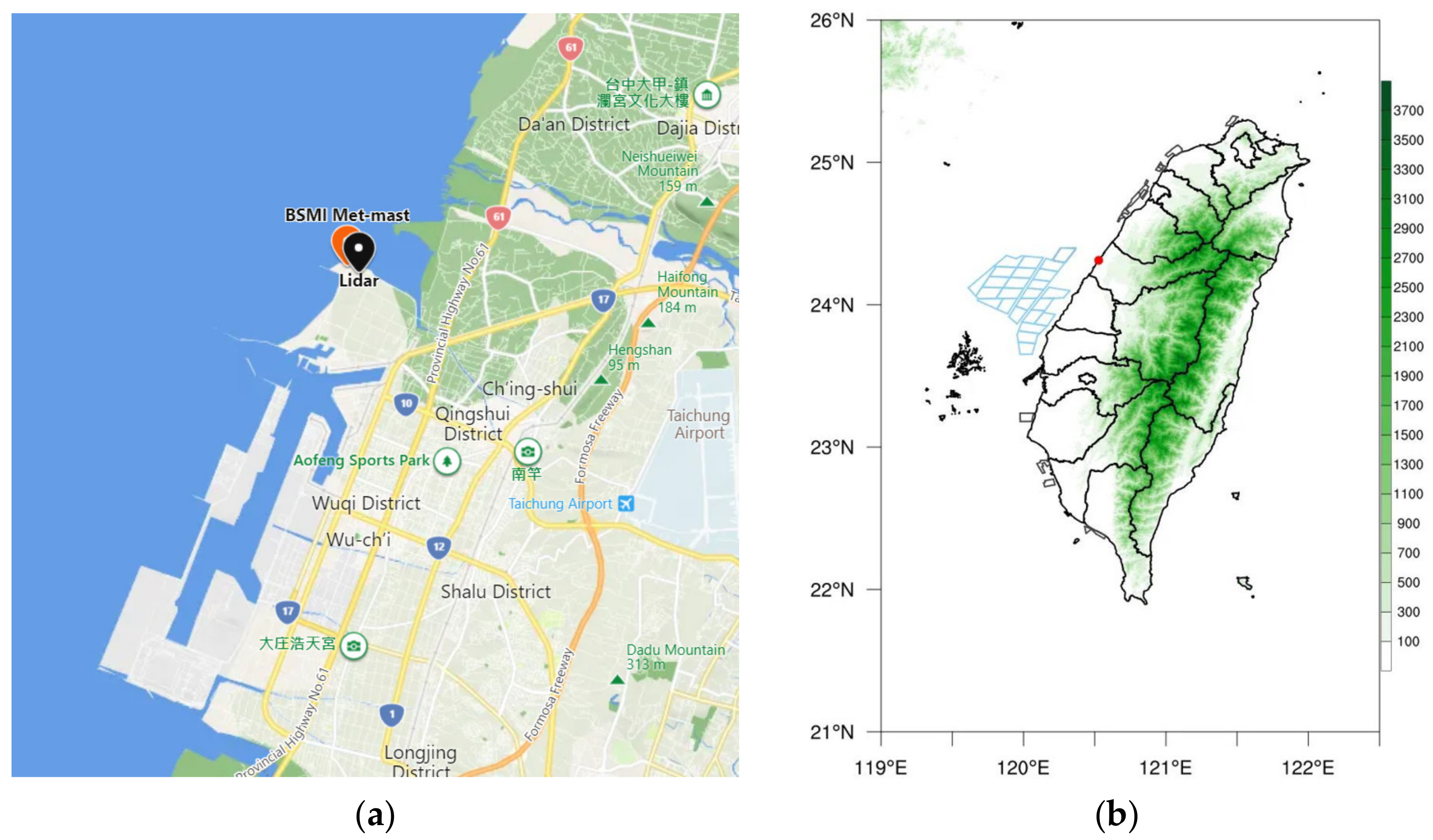
2. Data and Methods

Two data sources were used in this study. Wind speed data from 1 March 2016 to 31 December 2019, of the met mast of the Bureau of Standards, Metrology, and Inspection (BSMI) were used for the statistical modeling of wind speed. The mast is located on the coastline of Central Taiwan with anemometers installed at elevations of 100, 69, and 38 m, respectively. In 2019, the Central Weather Bureau observed wind speed by using a lidar at 400 m southeast of the mast. The highest elevation of the lidar can reach up to 200 m, providing wind speeds (including horizontal speed and direction, and vertical speed) at 12 levels (200, 175, 150, 125, 100, 82, 65, 48, 39, 25, 11, and 1 m, respectively) in approximately 18 s each. Therefore, the data provided additional characteristics of wind speeds such as the higher resolution of variation in wind profiles and the vertical component of wind. The data were used to verify the classification of sea breeze types. However, the measurements were performed only two times with approximately 1 month for each measurement. We analyzed the observation data in April 2019 and from 14 September to 13 October 2019, hereinafter referred to as 2019s and 2019a, respectively. Figure 1a shows the location of the met mast (red pin) and lidar (black pin). Figure 1b shows the map of Taiwan. The red dot represents the position of the met mast and lidar. The offshore blue grid is the main area of offshore wind farms in Taiwan.

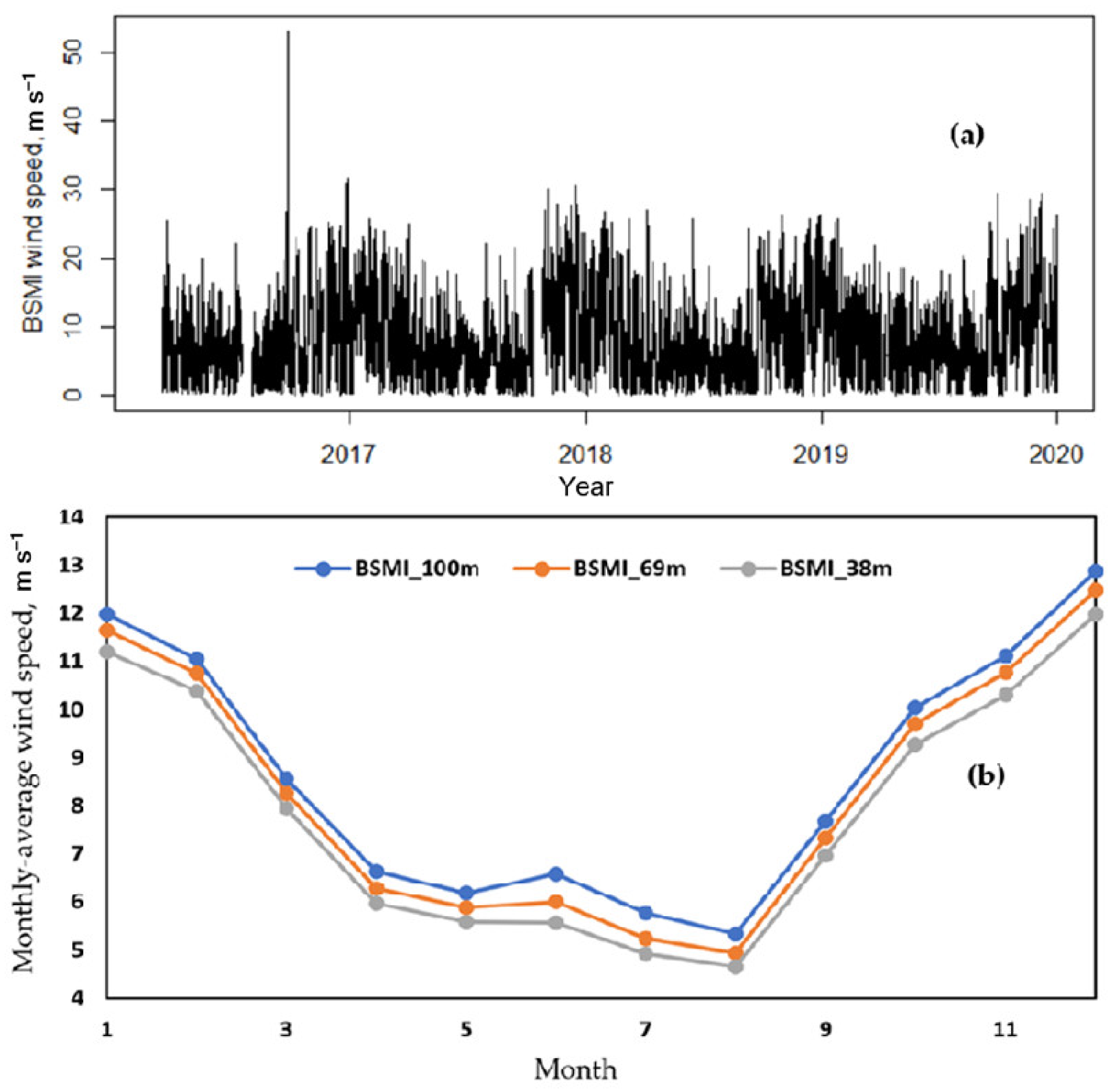
2.1. Wind Speed Characteristics

The BSMI wind speed observations span nearly 4 years. The 10 min average wind speed data were used to study the wind speed characteristics. Figure 2 shows the wind speed (at 100 m elevation) duration curve which represents the percentage of time a wind speed is exceeded. Considering a cut-in wind speed (minimum wind speed for the wind turbine to operate) of 4.0 m s⁻¹ and a cut-out wind speed (maximum wind speed before turning off the wind turbine for equipment protection) of 25 m s⁻¹, the wind turbine operating probability (the proportion of time for turbine operation) is approximately 0.75.

A time series plot of the observed wind speed at 100 m height is shown in Figure 3a. A cyclic pattern can be observed, indicating the presence of a non-stationary component in the wind speed time series. Figure 3b illustrates the temporal variation pattern of monthly average wind speed at different heights. Although the wind speed varies with height, their monthly variation patterns are similar. Wind speeds are high in mid-autumn to winter (October to February) and low in mid-spring to summer (April to August), with March and September being the transition period. The monthly wind speed pattern implies an annual cycle of wind speed.

In addition to the annual cycle, many observational and modeling studies also found that wind speed series display a distinct diurnal variation pattern which is driven mainly by the daily cycle of solar radiation at the top of the atmosphere [20,21]. In many studies, periodic components in the wind speed data series were identified or explained by visual interpretation of the monthly average wind speed plot or diurnal wind speed plot, without a mathematical formulation of the periodic components [21,22,23]. Other studies used time-invariant, linear autoregressive moving average (ARMA) models [24,25] or a time-varying autoregressive model [26], without an explicit expression of the periodic components, to simulate and forecast wind speed.

Since only less than 4 years of wind speed data is available for our study, we do not consider the increasing or decreasing trend in the observed data series. Thus, in our time series modeling, only the periodic components and a stationary residual series (upon removal of the periodic components) were considered. We aim to build a time series model which is composed of the periodic components and the stationary ARMA component for wind speed data series. Periodic components that may exist in a data series can be identified by its periodogram, instead of visual interpretation of the monthly average wind speed plot or diurnal wind speed plot.

In spectral analysis, a time series can be expressed as a sum of sinusoidal waves of various frequencies and amplitudes. The periodogram is a graph of frequencies and amplitudes which can be used to identify dominant frequencies that may explain the oscillation pattern of the observed data series. If a time series data is observed on a $\Delta t$ interval (for example, 10 min in our study) and its periodogram has a dominant spike at the frequency $f_o$, then the data series has a cyclic component of the period $\left(\frac{1}{f_o}\right)\Delta t$. The wind speed time series model which consists of a nonstationary periodic component and a stationary component is thus expressed by

$$X\left(t\right)=a_0+{{\displaystyle \sum }}_{k=1}^m[a_{k}Cos\left(2\pi f_{k}t\right)+b_{k}Sin\left(2\pi f_{k}t\right)]+Y\left(t\right)$$

(1)

where Y(t) is the stationary component that will be modeled as an ARMA process.

Figure 3. (a) Time series plot of the 10 min average BSMI wind speed at 100 m height. (b) Monthly wind speed at different heights.

Figure 3. (a) Time series plot of the 10 min average BSMI wind speed at 100 m height. (b) Monthly wind speed at different heights.

2.2. Types of Sea Breezes

According to the conditions of PW, sea breeze can be divided into three categories: pure sea breeze, corkscrew sea breeze, and backdoor sea breeze. Pure sea breeze occurs when light seaward PW is at a right angle to the coastline. Before the formation of sea breeze, the synoptic pressure gradient force (PGF) and the locally thermal PGF are briefly balanced, generating a calm zone. When PW has an along-shore wind component and the land is on the left (right), corkscrew (back door) sea breeze will be generated.

When PW has both along-shore and cross-shore components, corkscrew or backdoor sea breeze will be generated; these breezes can be distinct due to the effect of the Coriolis force and the difference in surface friction. Corkscrew sea breeze forms a divergent area near the coast (Figure 4a); hence, air from a high altitude can easily sink into the divergent area, resulting in the formation of sea breeze. Because the thermal and synoptic PGF are not completely in the same dimension, the thermal PGF does not have to overcome all the magnitudes of the synoptic PGF. Hence, no calm zone is formed before the sea breeze begins [11]. This indicates that a weaker PGF than that required for generating pure sea breeze would be adequate to form corkscrew sea breeze. Likewise, backdoor sea breeze (Figure 4b) will form a convergence zone near the coast, making it difficult for air at high altitudes to sink and inhibiting the movement of sea breeze toward the land. Thus, compared with pure or corkscrew sea breeze, backdoor sea breeze requires a stronger thermal PGF to reach the coast.

2.2.1. The Ellipse and Average Vector Composite Hodograph (Abbreviated as EACH) Method: A New Identification Method for Sea Breeze Types

Because an idealized sea-breeze hodograph has an elliptical shape [27], a new method based on an elliptical shape for identifying types of sea breeze was proposed. After analyzing lidar data from the Central Weather Bureau, we suggested a new effective and convenient method to classify the types of sea breeze and estimate the magnitude of PW and sea breeze components. We named this as the ellipse and average vector composite hodograph (abbreviated as EACH) method.

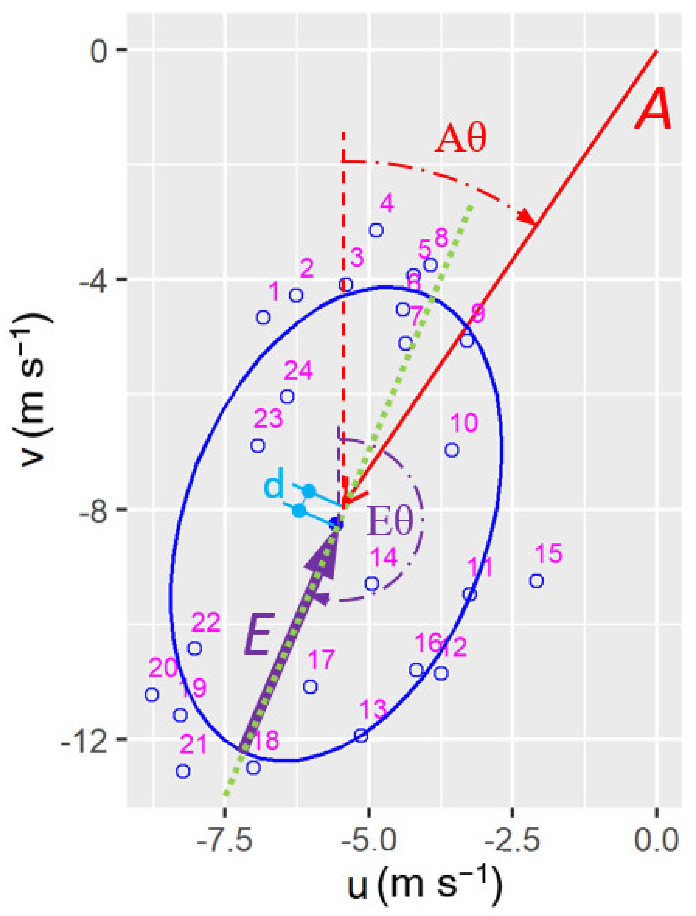
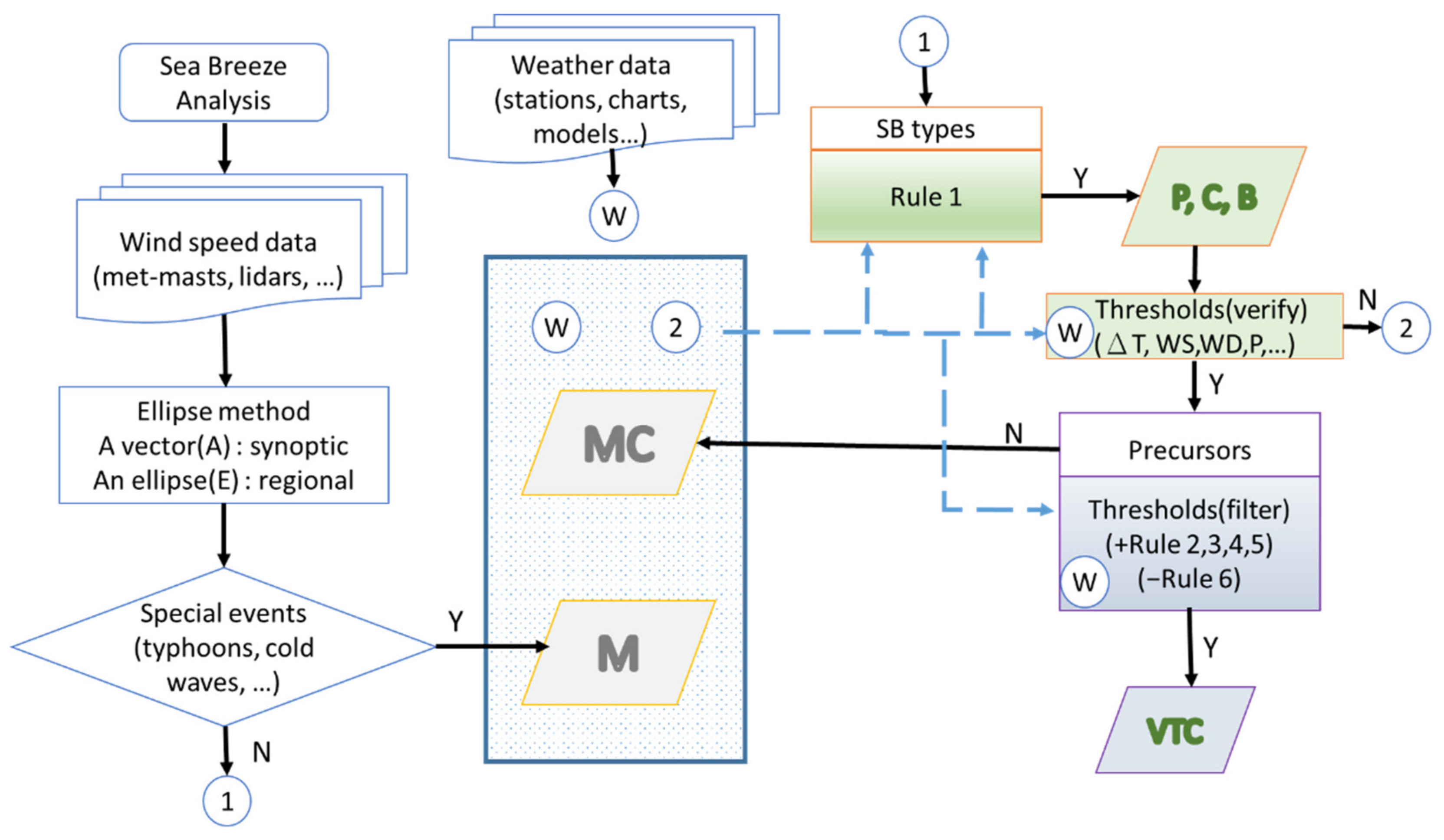
2.2.1.1. Specific Steps of This Method Are as Follows (Figure 5)

• Developing a hodograph with hiding vectors and no connections among the arrowheads of vectors for the purpose of clearness;
• Marking the arrowheads (e.g., blue circles);
• Adding the average velocity vector (denoted by A in Figure 5). Its magnitude and direction are represented by Av and Aθ, respectively;
• Fitting all velocities with an ellipse to obtain the length and angle of the semi-major axis (denoted by E in Figure 5). Magnitude and direction of E are represented by Ev and Eθ, respectively.

2.2.1.2. Main Ideas of the Plotting Method Are as Follows

• In the velocity diagram, the PW vector is replaced by an average wind vector (A);
• Wind speeds in a day at the same altitude are fitted by an ellipse;
• Identification of the sea breeze type depends on the angle among the average wind vector and the coastline;
• Weather conditions of candidates are used to verify whether the identification of the sea breeze type is correct (rules introduced in the next section);

During the process,

• Thresholds of environmental variables (such as the temperature difference) of each sea breeze type can be set up;
• Conditions for candidates of maximum and minimum values on a certain time scale (such as the month and season) are analyzed, and these conditions might predict the sea breeze type and velocity.

Figure 5. An ellipse example (on 15 September 2019); The red solid line with an Italic A denotes the average wind vector. Its meteorological direction is Aθ. The blue solid line denotes a fitted ellipse. The purple solid line with an Italic E denotes the semi-major axis with a meteorological direction (Eθ). The distance between the arrowhead of A and the center of the ellipse (the blue dot) is denoted by d in sky-blue. Blue circles under magenta digits denote hourly mean wind vectors of the local time.

Figure 5. An ellipse example (on 15 September 2019); The red solid line with an Italic A denotes the average wind vector. Its meteorological direction is Aθ. The blue solid line denotes a fitted ellipse. The purple solid line with an Italic E denotes the semi-major axis with a meteorological direction (Eθ). The distance between the arrowhead of A and the center of the ellipse (the blue dot) is denoted by d in sky-blue. Blue circles under magenta digits denote hourly mean wind vectors of the local time.

3. Results

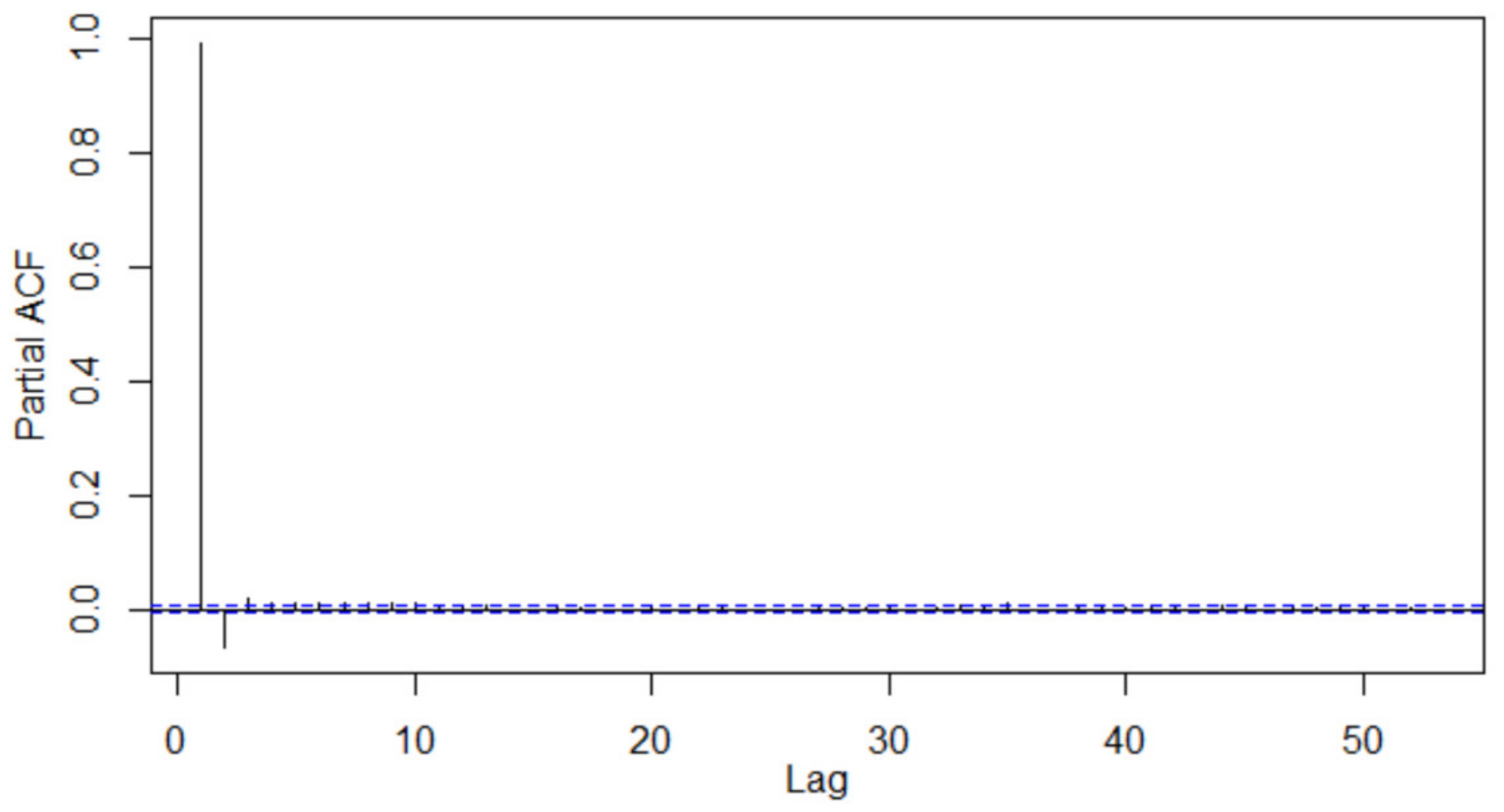
3.1. Time Series Modeling of the Wind Speed

In this study, both the frequency-domain and time-domain characteristics of the wind speed data series were considered. Our time series modeling approach consists of two steps: (1) frequency domain—identifying the periodic components by the spectral analysis; (2) time domain—building an ARMA model for the residual time series (Y(t) in Equation (1)). The periodogram of the 10-min average wind speed at 100 m height is shown in Figure 6. In a periodogram, the frequency should span over 0 to 0.5. We only show the periodogram within the [0, 0.02] frequency range since the spectrum values are very low beyond that range. Two peaks at the frequencies (in unit of cycles per 10-min) $f_1=1.9753\times {10}^{-5}$ and $f_2=6.94444\times {10}^{-3}$ were identified. The two peak frequencies correspond to the periods of 352 days and 1 day, respectively. Considering the relatively short observation period, we chose to set two periodic components with periods of 365 days and 1 day, respectively.

The amplitudes of the two periodic components ($a_k \mathrm{and} b_k$ in Equation (1)) were then determined by linear regression (see

Table 1. Parameters of the time series model of wind speed at 100 m height. The time series model is expressed by Equations (1) and (2).

Nonstationary component	$a_0$	$a_1$	$b_1$	$a_2$	$b_2$
	8.62636	1.44623	−3.04006	−0.89615	−1.04959
Stationary component AR(3)	${\alpha }_1$	${\alpha }_2$	${\alpha }_3$	${\sigma }_{ϵ}^2$
	1.00619	−0.0887	0.0192	0.3464

). Figure 7a demonstrates that the yearly seasonal variation pattern of wind speed can be well described by the frequency $f_1$. Figure 7b shows the diurnal variation pattern ($f_2$) embedded in the seasonal variation pattern.

Figure 6. The periodogram of 10 min average wind speed at 100 m height.

Figure 6. The periodogram of 10 min average wind speed at 100 m height.

The diurnal variation pattern of the wind speed is difficult to observe in Figure 7a, since the data series was squeezed. We analyzed the monthly diurnal variation pattern by calculating the average wind speed of individual hours for each month. The wind speed diurnal variation patterns of individual months and their annual average are depicted in Figure 8a. Although there seems to be a common diurnal variation pattern with wind speed peaks in the afternoon, the hours of peak occurrence of the high wind-speed months (October to February) are about 2 to 3 h later than that of the low wind-speed months (April to August). The wind-speed variation range is larger in the high wind-speed season than in the low wind-speed season. The hourly wind speeds of 25 August and 25 December 2016 (see Figure 8b,c) exemplify the above characteristics.

After the nonstationary periodic components were identified, they were removed from the observed wind speed series, and the residual series was treated as an ARMA series. Previous studies have shown that autoregressive (AR) model is appropriate for wind speed data [24,25]. An AR model of lag order k can be expressed by

$$Y\left(t\right)={\alpha }_{1}Y\left(t-1\right)+{\alpha }_{1}Y\left(t-2\right)+\cdots +{\alpha }_{k}Y\left(t-k\right)+ϵ\left(t\right)$$

(2)

where $ϵ\left(t\right)$ represents the noise which has a normal distribution of zero expectation and variance ${\sigma }_{ϵ}^2$. For an AR(k) random process, its theoretical partial autocorrelation coefficients are equal to zero beyond k lags. Thus, the lag order of an AR model can be identified by the partial autocorrelation function (PACF) of the data series.

Figure 9 shows the PACF plot of the residual series, together with the 95% confidence interval (blue dashed lines) of the partial autocorrelation coefficients. The PACF values fall within the 95% confidence interval for lags higher than 3. Thus, the residual series is modeled as an AR(3) model. Estimates of the AR(3) model parameters are listed in Table 1.

The established time series model combining the nonstationary periodic component (Equation (1)) and the AR model (Equation (2)) can be used for short period wind speed forecasting. Figure 10 illustrates an example of a 1-step lead-time wind speed forecast. The mean absolute error (MAE) and root mean squared error (RMSE) of the wind forecasts are 0.32 $\mathrm{m}·{\mathrm{s}}^{-1}$ and 0.43 $\mathrm{m}·{\mathrm{s}}^{-1}$, respectively. The proposed time series model yields good short period forecast results.

Figure 9. The partial autocorrelation function of the residual series.

Figure 9. The partial autocorrelation function of the residual series.

3.2. Case Study for the Application of the EACH Method

The EACH method was applied to the 2019s and 2019a data, taking the wind speed at a height of 100 m as an example. The following results were obtained. Data retrieved at 1 m height were excluded because of the presence of various ground activities and the considerable distance to the wind turbine’s blades.

In the velocity diagram, the average distances in 2019s and 2019a between the arrowhead of the average wind vector and the center of the ellipse (denoted by d in Figure 5) were 1.23 and 0.6 m s⁻¹, respectively. The standard deviations were 0.81 and 0.42 m s⁻¹, respectively. Meanwhile, the means of average wind vectors (A) in the two datasets were 5.76 and 9.76 m s⁻¹, respectively. The accuracy of the average wind vectors was sufficient for the purpose of identification.

3.2.1. Rules

The following rules were concluded from the cases, where rule 1 was for sea breeze type identification. Rules 2–5 were for finding candidates that changed the trend of wind speed. Rule 6 was for the absence of sea breeze.

Before processing data, extreme events such as typhoons should be excluded and analyzed separately. For example, Typhoon Mitag passed by on 30 September 2019, resulting in two days of high winds, followed by two days of low winds due to high pressure. Common rules could not be applied to the directions and angles of A and E during this event.

Rules were as follows in this study:

1.

The angle between A and the coastal line determines the type of sea breeze due to the presence of the along-shore component, as mentioned in Section 2.2;

1a.

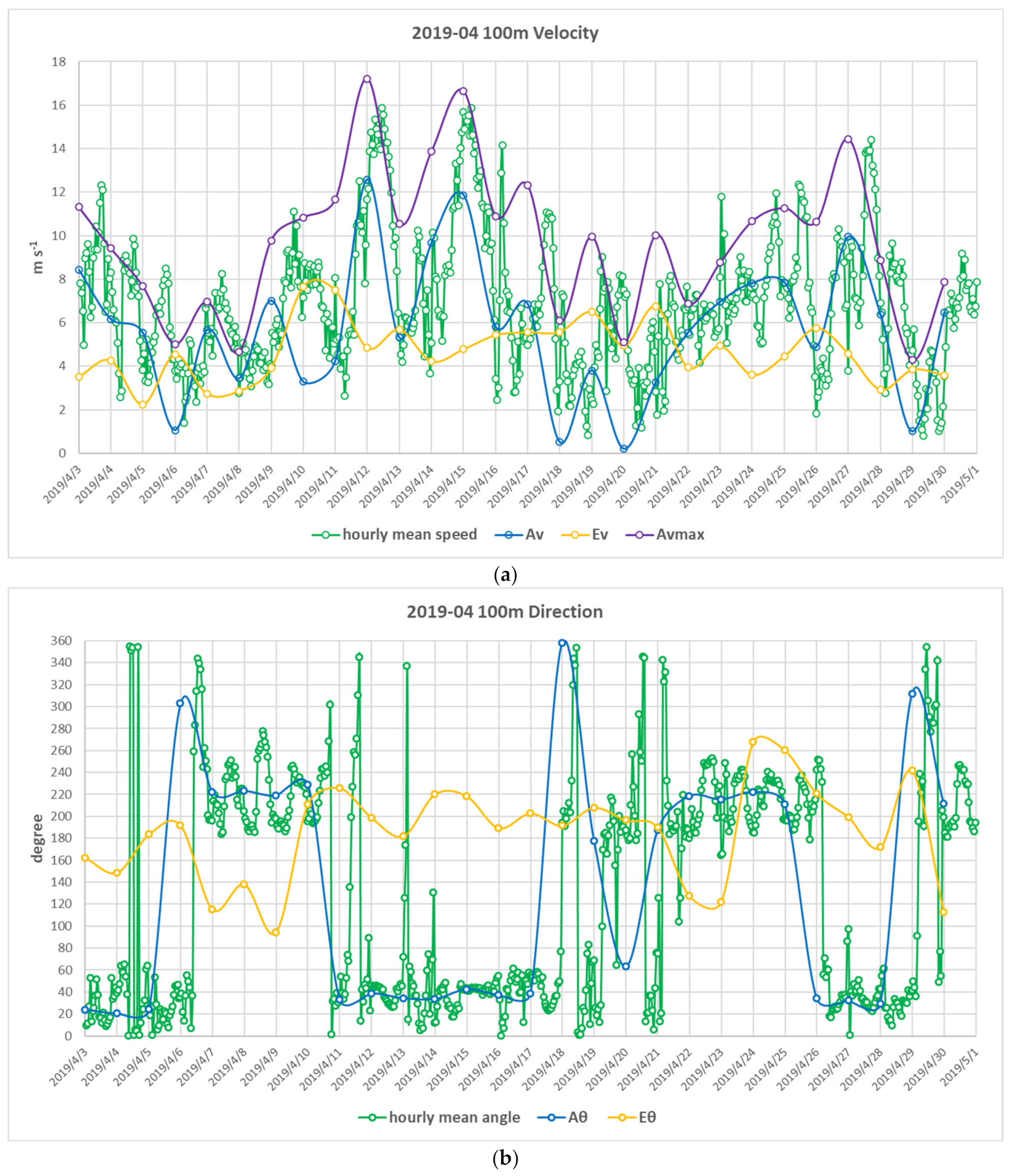
Pure sea breeze occurs in weak synoptic PGFs. A approached the coastal line at a right angle (at some 300°, Figure 11);

1b.

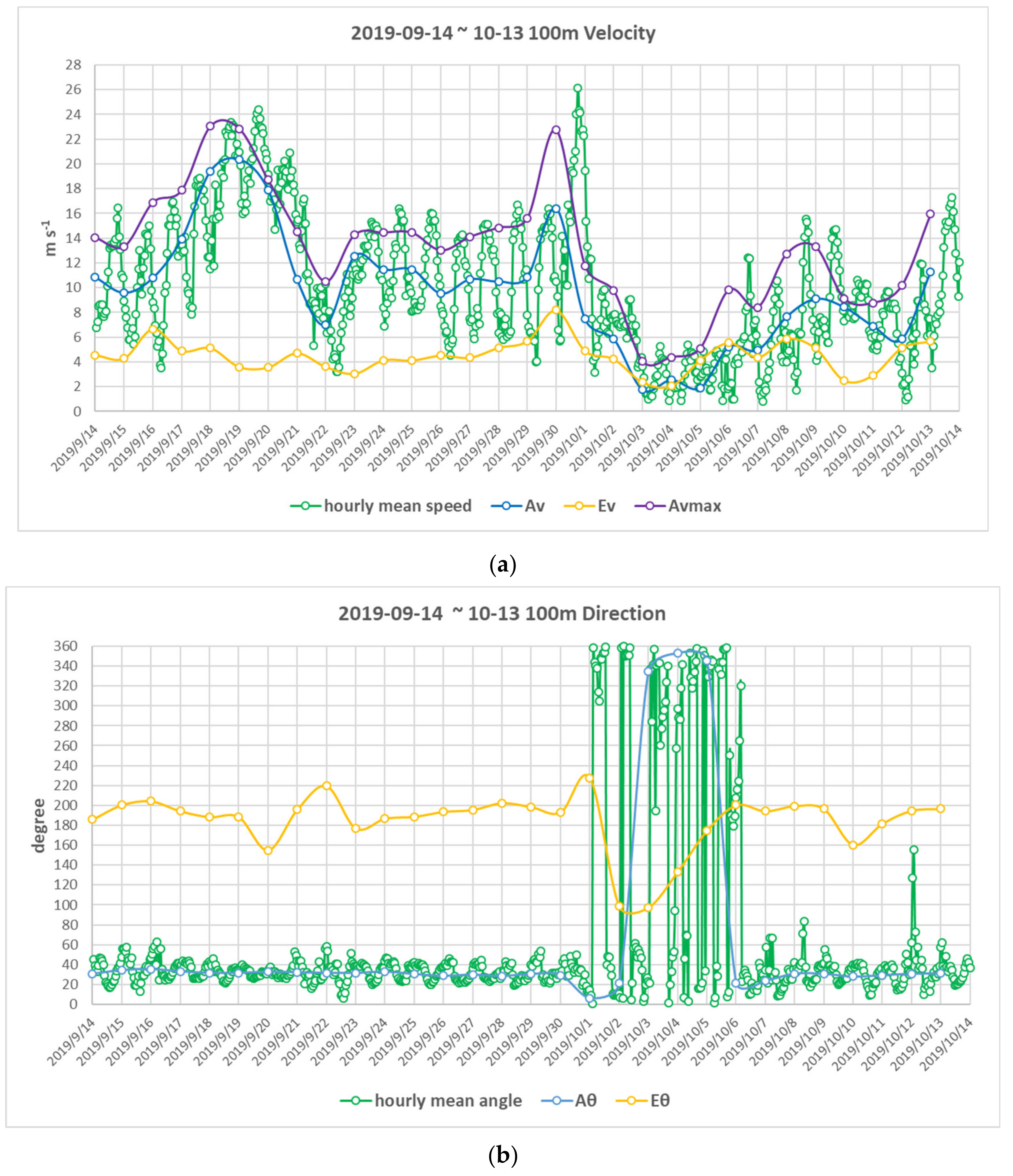
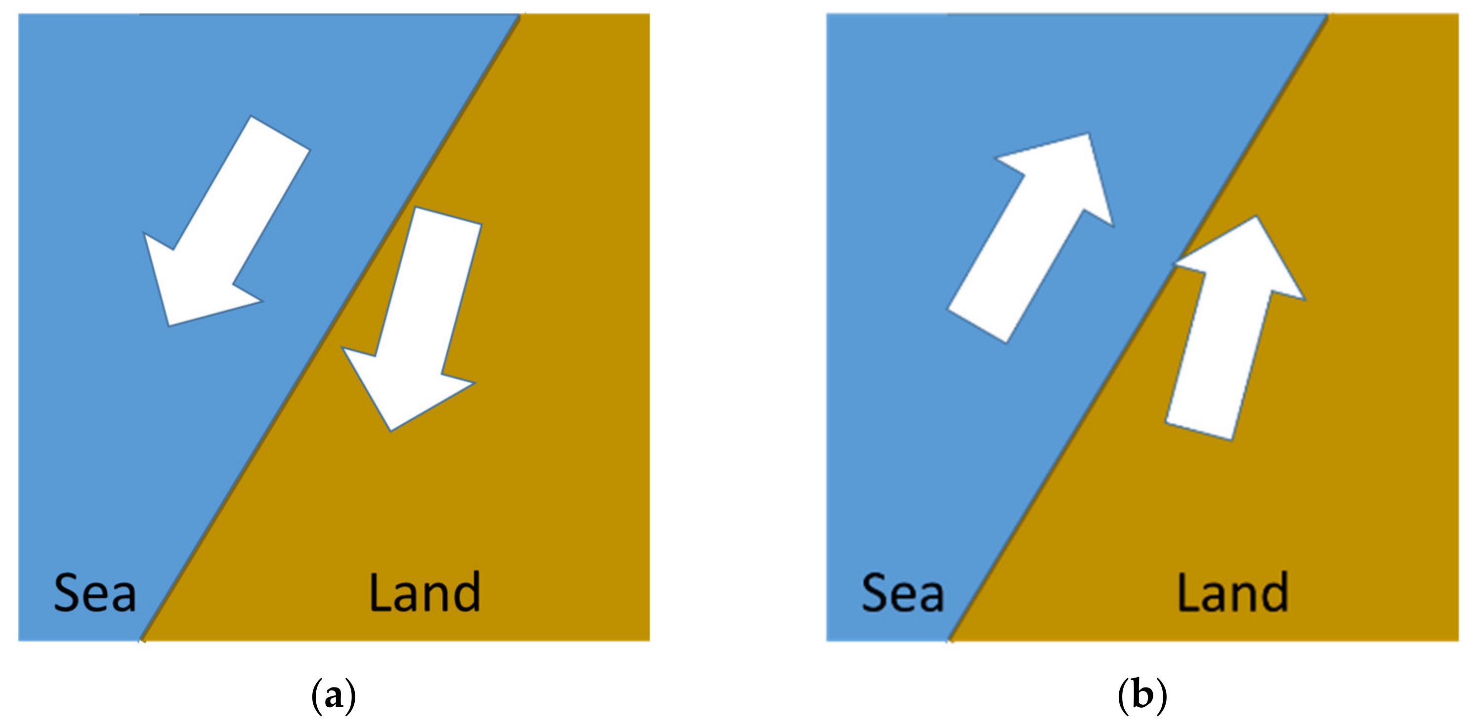
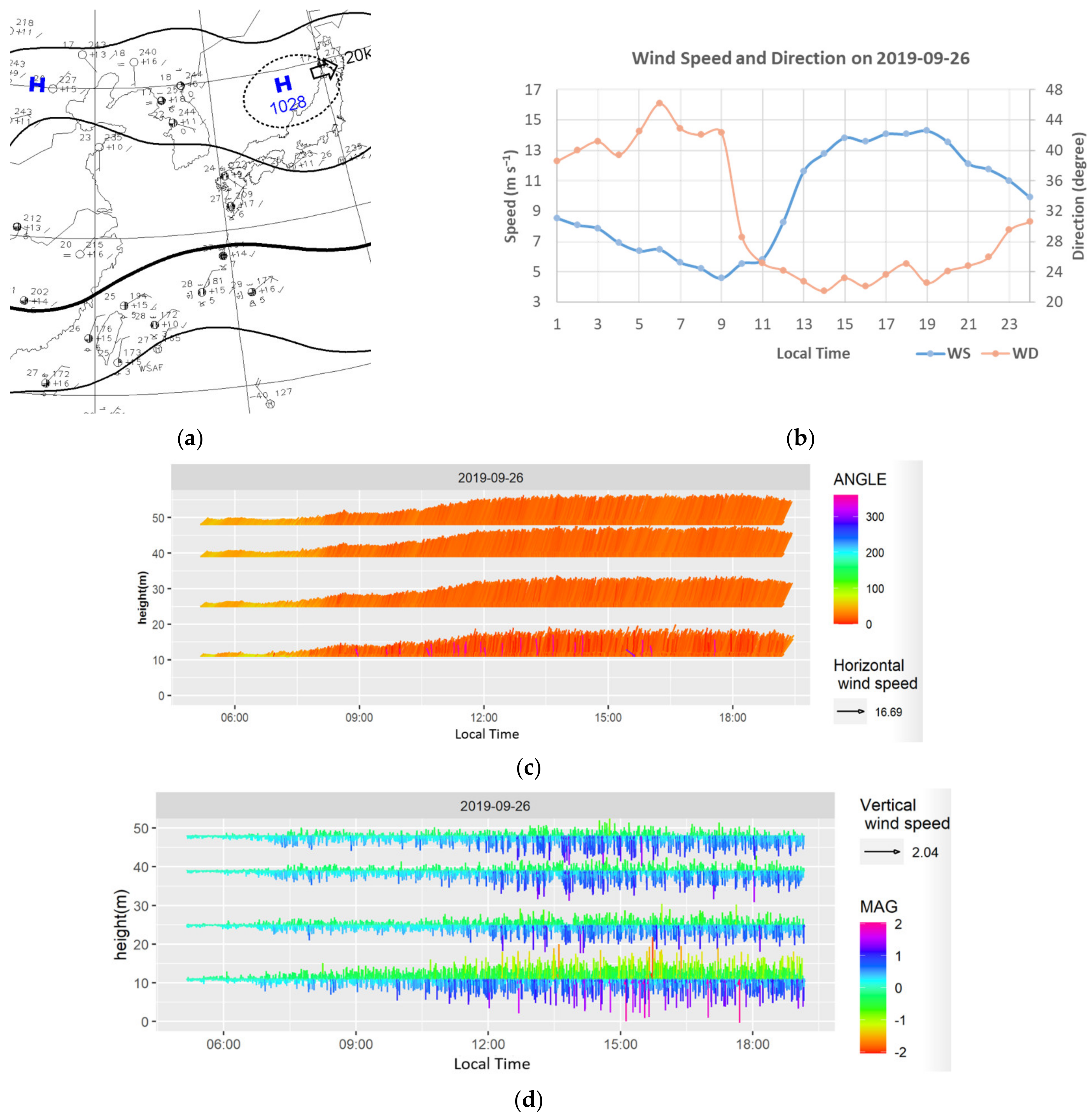
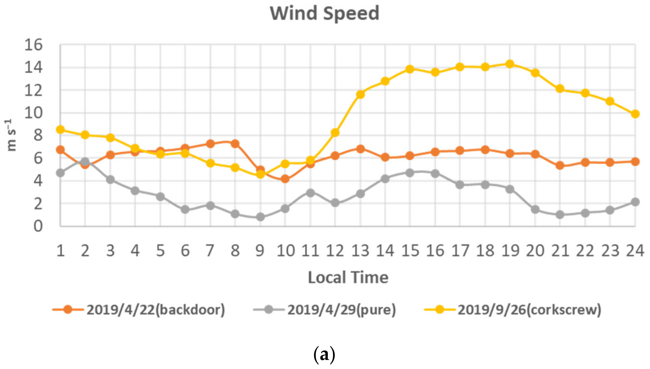
Corkscrew sea breeze occurs when A comes from the north ranging from 120° to 300° (counterclockwise in Figure 11). The presence of an along-shore component with land on the left caused a divergent area, resulting in the easy sinkage of high-altitude air. Usually, the daily peak of wind speed occurs in the late afternoon;

1c.

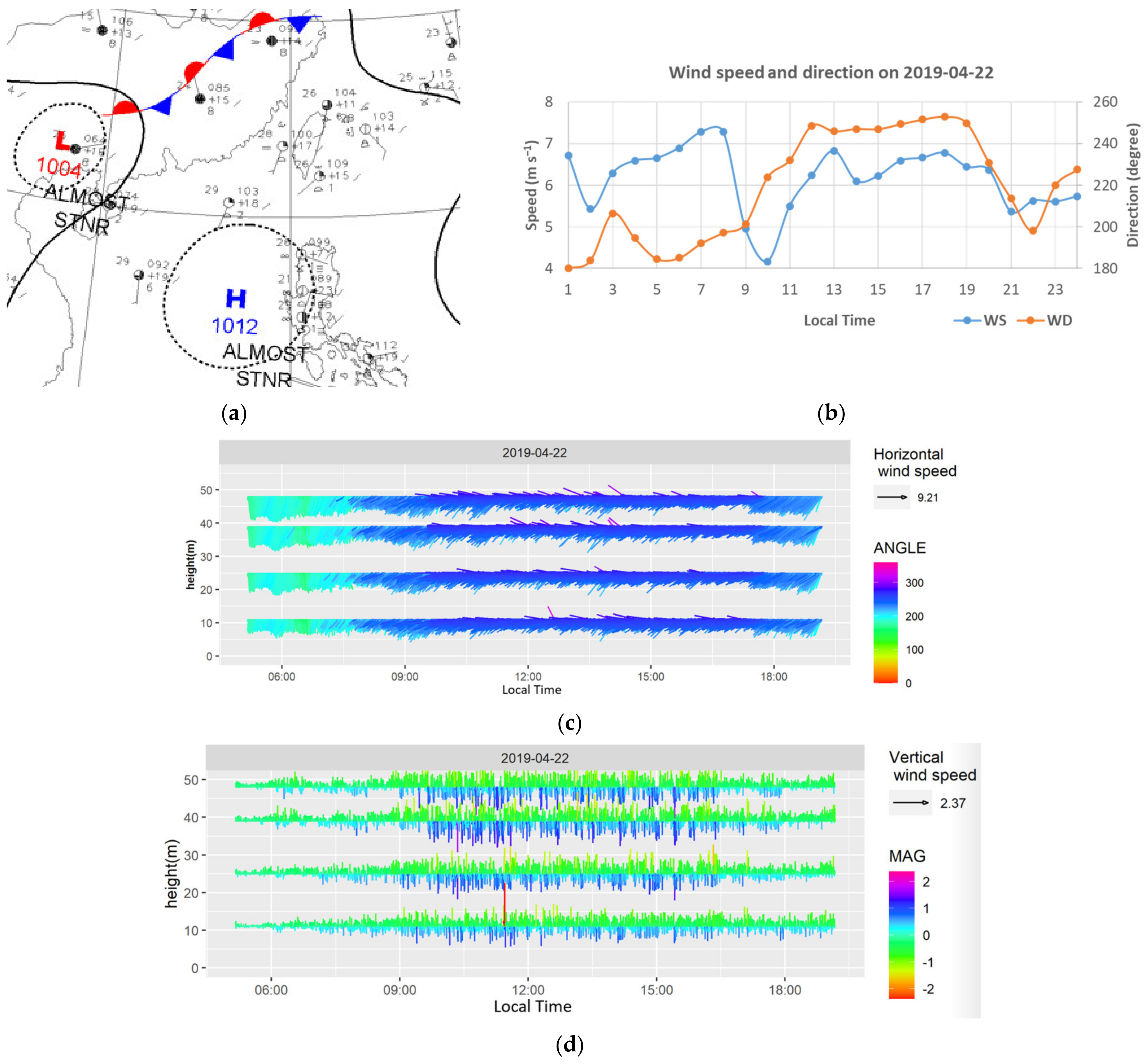
Backdoor sea breeze occurs when an along-shore component comes from the south and A ranges from 120° to 300° (clockwise in Figure 11). The development of a convergent area inhibited the sinkage of high-altitude air. Usually, the daily peak of wind speed occurs around noon.

Figure 11. Schematic diagram of the observation site.

Figure 11. Schematic diagram of the observation site.

The following results were obtained after classification (

Table 2. Results of sea breeze type identification in case 2019s and 2019a. (Each cell represents a day with date inside, the text in square brackets show the rules that were met.)

	4/11 [1b,4]	4/21 [1c,4]	9/14 [1b]	9/24 [1b,4]	10/4 [1b,2]
	4/12 [1b,4]	4/22 [1c]	9/15 [1b,4]	9/25 [1b,4]	10/5 [1b,2,4]
4/3 [1b]	4/13 [1b]	4/23 [1c]	9/16 [1b,4]	9/26 [1b,4]	10/6 [1b,4]
4/4 [1b]	4/14 [1b,4]	4/24 [1c]	9/17 [1b,4]	9/27 [1b,4]	10/7 [1b,4]
4/5 [1b]	4/15 [1b,4]	4/25 [1c]	9/18 [1b]	9/28[1b,4]	10/8 [1b,4]
4/6 [1a]	4/16 [1b]	4/26 [1b,4]	9/19 [1b]	9/29 [1b,4]	10/9 [1b,4]
4/7 [1c]	4/17 [1b,4]	4/27 [1b,4]	9/20 [1b]	9/30 [1b,4]	10/10 [1b]
4/8 [1c]	4/18 [1b,4]	4/28 [1b]	9/21 [1b,4]	10/1 [1b]	10/11 [1b]
4/9 [1c]	4/19 [1c,3]	4/29 [1a]	9/22 [1b,4]	10/2 [1b]	10/12 [1b,4]
4/10 [1c,4]	4/20 [1c,2]	4/30 [1c]	9/23 [1b,4]	10/3 [1b,2]	10/13 [1b,4]

Colors in cells represent sea breeze types: yellow—pure; blue—corkscrew; green—back-door; brown—special event.

). The first two cells are left blank because of no observation. The colors filled in cells represent the type of sea breeze: yellow is for pure sea breeze, blue is for corkscrew sea breeze, and green is for backdoor sea breeze. Brown cells denote special events; for example, on 4/15, sea breeze may be suppressed and cannot be generated. Typhoon Mitag was from to 30 September to 4 October. The text in the square brackets of cells show the rules that were met.

2.

In corkscrew sea breeze, when the included angle between A and the coastline (approximately 60° with respect to the zonal direction) was greater than 30° (i.e., beyond [0, 60] in Figure 11), the extent of divergence and the speed of wind were decreased due to the decreased projection of wind speed onto the coastline. For example, included angles, from 10/3 to 10/5, between A and the coastline were greater than 30° (Figure 12);

3.

In backdoor sea breeze, when the included angle between A and the coastline was greater than 30° (i.e., beyond [180, 240] in Figure 11), the extent of convergence was decreased due to the decreased projection of wind speed onto the coastline. The wind speed increased. For example, 4/19 (Figure 13);

4.

The minimum included angle between A and E, ignoring the orientation of vectors due to the symmetry of ellipses, was within ±20°. Under this situation, either the summation or subtraction of Av and Ev can be the candidate changing the trend of speed. Based on the surface weather chart of the studied cases, the situation was probably caused by a nearby weather system, such as fronts, depressions, and high pressures, resulting in a larger variation (more than 180°) in wind direction. During the average process of vectors, a large direction variation was likely to offset each other, resulting in unusual but similar angles;

5.

The possible maximum speed of the day (Avmax) might be obtained by applying the law of cosines to Av and Ev. The variation in the velocity curve (Avmax) was in phase with that of hourly wind speeds, thus providing useful vertices of curves (refer to purples lines in Figure 12 and Figure 13);

6.

If the semi-minor axis of the ellipse was less than 1 m/s and the minimum included angle between A and E, ignoring the orientation of vectors due to the symmetry of ellipses, was within ±10°, sea breeze may be suppressed. For example, 4/15 (as shown in Figure 13).

Figure 12. (a) Wind speed variation during 14 September–13 October 2019; (b) Wind direction variation during 14 September–13 October 2019. The green line is for the hourly mean wind vector. The blue line is for vector A. The yellow line is for vector E. The purple line is for the possible maximum wind vector of the day.

Figure 12. (a) Wind speed variation during 14 September–13 October 2019; (b) Wind direction variation during 14 September–13 October 2019. The green line is for the hourly mean wind vector. The blue line is for vector A. The yellow line is for vector E. The purple line is for the possible maximum wind vector of the day.

Figure 13. (a) Wind speed variation in April 2019 (b) Wind direction variation in April 2019. The green line is for the hourly mean wind vector. The blue line is for vector A. The yellow line is for vector E. The purple line is for the possible maximum wind vector of the day.

Figure 13. (a) Wind speed variation in April 2019 (b) Wind direction variation in April 2019. The green line is for the hourly mean wind vector. The blue line is for vector A. The yellow line is for vector E. The purple line is for the possible maximum wind vector of the day.

3.2.2. Verification

The lidar data and surface weather chart were used to verify breeze types identified using the EACH method. The verification of selected days is shown due to limited space. The time shown on the surface weather chart is UTC, and the local time in Taiwan is 8 h ahead of UTC. The arrowhead of the wind speed vector on the lidar data diagram indicates the horizontal line representing its height. The color bar legend on the horizontal wind speed component diagram is for wind direction. The color bar legend on the vertical wind speed component diagram is for wind speed. The scales in each figures are different due to limited space.

• Pure sea breeze on 6 April 2019

As shown in Figure 14a, the high-pressure center moved eastward and was about to dissipate, resulting in the diminishing effect of high-pressure circulation on the western coastal area of Taiwan. No other synoptic weather systems were noted in the Taiwan Strait. At the height of 11 m (sea breeze began from the surface), some vertical speed components equal zero and horizontal speed components close to zero (Figure 14c,d) indicating a calm zone developed from 0500 to 0700 local time. Wind direction varied frequently, and no PW dominated. To sum up, this was a pure sea breeze day.

• Corkscrew sea breeze on 26 September 2019

As shown in Figure 15a, the high-pressure center in the north made the wind field around Taiwan northeasterly. No calm zone was noted. As the divergence zone developed over the coastal area in the morning, which encouraged subsidence [11], the vertical component (refer to the green subsided vectors in Figure 15d) of the wind speed reached the maximum in the late afternoon as expected. In the meantime, the horizontal wind component affected by PW kept accelerating and rotating counterclockwise in the daytime.

• Backdoor sea breeze on 22 April 2019

On the west side of Luzon Island, a dissipating high pressure made the wind field around Taiwan southwesterly (Figure 16a). No calm zone was noted. As the convergence zone developed, the subsidence over coastal areas was suppressed. Consequently, although the horizontal wind component, which was affected by PW, continued to rotate clockwise, it appeared a bit jolting (winds veered with frequently backed in between). Speed decreased first and then increased, as shown in Figure 16b,c. Figure 16d shows that vertical wind speeds reach their maximum value of the day around noon as expected for the backdoor sea breeze.

• A special event on 15 April 2019 for rule 6.

Figure 17a shows a small included angle between A and E. In addition, a small semi-minor axis of the ellipse is depicted. A steady wind direction curve is shown in Figure 17b. Both the surface weather chart and lidar data showed an average day of northeasterly wind. However, the examination of surface temperatures (Figure 17c) indicated that the air temperature over the land (obtained from Jhunan automatic meteorological observation station) was lower than that over the sea surface (obtained from Hsinchu Buoy) during daytime, lacking the driving force to establish the thermal pressure gradient. As shown in Figure 17c, the orange line represents the normal condition of the previous day. The blue line shows the unusual condition due to a significant land temperature drop by the southward moving cold air from April 14 to 16. This is a rare situation considering that spring is usually the coldest season of the sea surface temperature in a year.

4. Discussion

4.1. The EACH Method

The advantage of the EACH method is to simplify the variation of wind speed in a day into a constant average wind and a semi-major axis of an ellipse, making the identification concise and effective. A computer code can be easily developed to process large amounts of data automatically.

In the flowchart (Figure 18), green cells are for sea breeze type identification. Purple cells are for the vertices of wind speed time series curve, which are the candidates of extremes and might be precursors for forecasting. The blue circle with W inside denotes weather data. In the beginning, weather data were analyzed to set up thresholds for verification and filtering. The blue cell with shading contained all rejected data. Manual analysis might help find new rules and thresholds to validate the original ones with regional characteristics (as shown by the blue dashed lines). P,C,B denotes pure, corkscrew, and backdoor sea breeze, respectively. VTC denotes vertices which are points that wind speed trend change in time series. M and MC denote manual processes required for processing data.

The procedures are as follows:

• Applying rule 1 to classify the sea breeze types on the dates of interest;
• Applying rules 2 to 6 to find the vertices of speed curves as the candidates of extreme points;

  ◦

  Filtering out dates that comply with rules 6;

  ◦

  Keeping dates that comply with rules 2, 3, 4, and 5;

• Analyzing the weather conditions of candidates with the same sea breeze type to verify the sea breeze types. At the same time, determining effective environmental variables and their thresholds. Analyzing these thresholds to determine factors that results in candidates to have extreme values at a specific time scale, which could be predictors of sea breeze velocity. Because only filtered data are processed, the EACH method can speed up the analysis.

The more data analyzed in the same area, the better the rules are established and more accurate and effective results can be obtained. In short, the EACH method was simple, convenient, scalable, and adaptive.

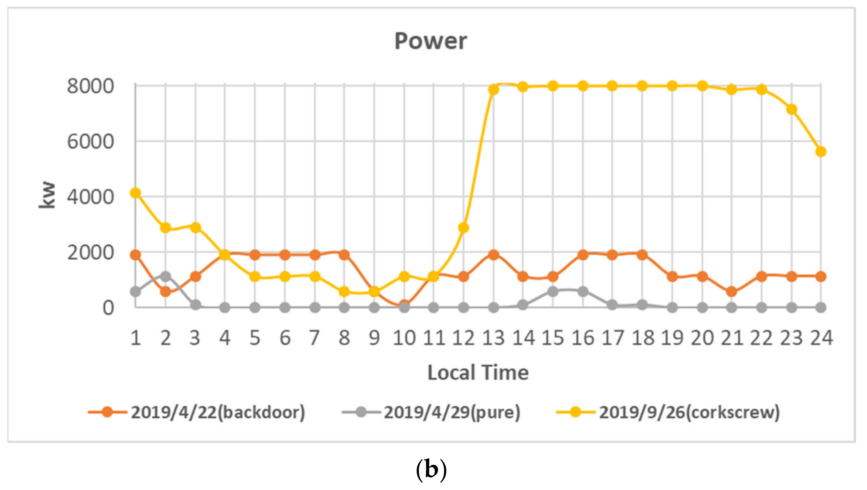
4.2. Daily Power Production of Each Sea Breeze Type

From the cases of 2019s and 2019a, the typical daily wind speed curve of each sea breeze type could be found by medians. The median of PW and the semi-major axis of the ellipse for corkscrew sea breeze were 9.07 and 4.57 m s⁻¹, respectively. Therefore, the wind-speed curve on September 26 was selected to simulate power generation. Likewise, the median of PW and the semi-major axis of the ellipse for backdoor sea breeze were 5.59 and 4.2 m s⁻¹, respectively. Therefore, the wind-speed curve on 22 April was selected to simulate power generation. Finally, the wind-speed curve on April 6 was selected to simulate the power generation of pure sea breeze.

We used the power curve of an 8-MW reference wind turbine with 4 m s⁻¹ cut-in speed and 25 m s⁻¹ cut-out speed from the EU FP7 project LEANWIND to calculate the daily production. The power curve is illustrated in Figure 19.

As shown in Figure 20b, a typical corkscrew sea breeze day can produce 114,000 kwh, whereas typical backdoor sea breeze day can produce 32,310 kwh. The typical pure sea breeze day can only produce 3380 kwh. The power produced by corkscrew sea breeze was 33.7 times that of pure sea breeze and 9.6 times that of backdoor sea breeze.

4.3. A Good Approximation of the Magnitude of Sea Breeze Speed

The EACH method is a simple and effective approximation method that can be used to identify the types of sea breeze and quantitatively evaluate sea breeze velocity. Determining the intensity of sea breeze is difficult when the weather system is strong.

In the case of 2019s, the average Av was 5.76 m s⁻¹ and the average Ev was 3.21 m s⁻¹. In the case of 2019a, the average Av was 9.76 m s⁻¹ and the average Ev was 3.17 m s⁻¹. The root sum squared of the average Av and the average Ev in cases 2019s and 2019a were 6.59 and 10.26 m s⁻¹, respectively. By contrast, the average of all the hourly mean velocities in those two cases were 6.9 and 10.01 m s⁻¹, respectively. The errors were only 0.31 and 0.25 m s⁻¹, respectively.

If we used the average Av to represent the component related to the synoptic-scale system and the average of Ev to represent the rotational component related to the regional system in the wind field, we can better understand the characteristics of wind speed and the features of speed variation in the wind field. These values can be used to compare wind fields at different locations or to determine why speed varies at different times in the same wind field.

5. Conclusions

Wind power is a promising renewable energy source. Taiwan, located in the subtropical zone and surrounded by the sea, is suitable for the development of offshore wind power. However, the random and intermittent nature of the wind and the time-varying direction of the land–sea breeze make balancing the power grid challenging. Moreover, based on our study, the daily power production of the corkscrew sea breeze was more than 33 times that of pure sea breeze and 9 times that of backdoor sea breeze. Therefore, Taiwan should conduct more research on sea breeze to foresee the occurrence of pure and backdoor sea breeze, especially on peak power demand hours.

This study established a wind speed statistical model for Central Taiwan to improve the accuracy of very short-term predictions. A new method was proposed that can effectively identify sea breeze types and quantitatively evaluate their magnitude.

Conclusions drawn from the study are as follows:

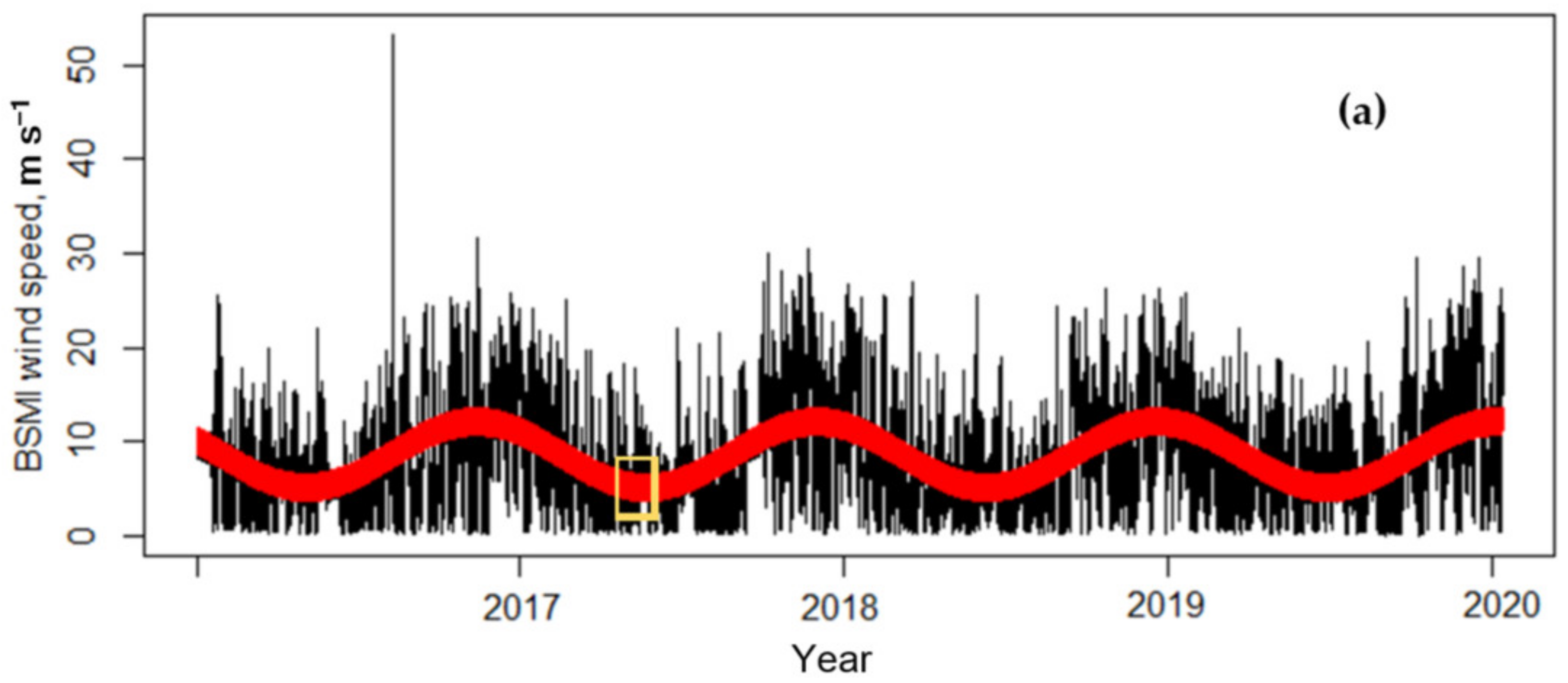
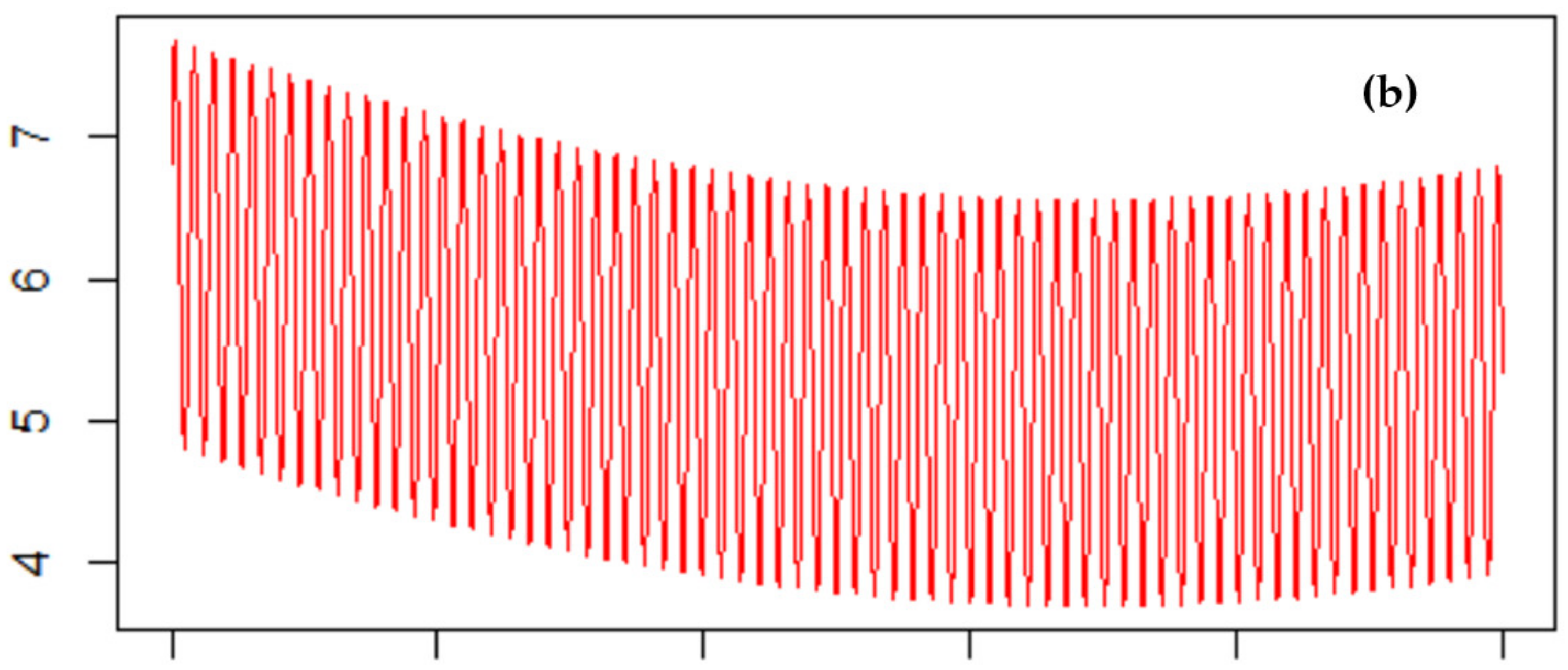
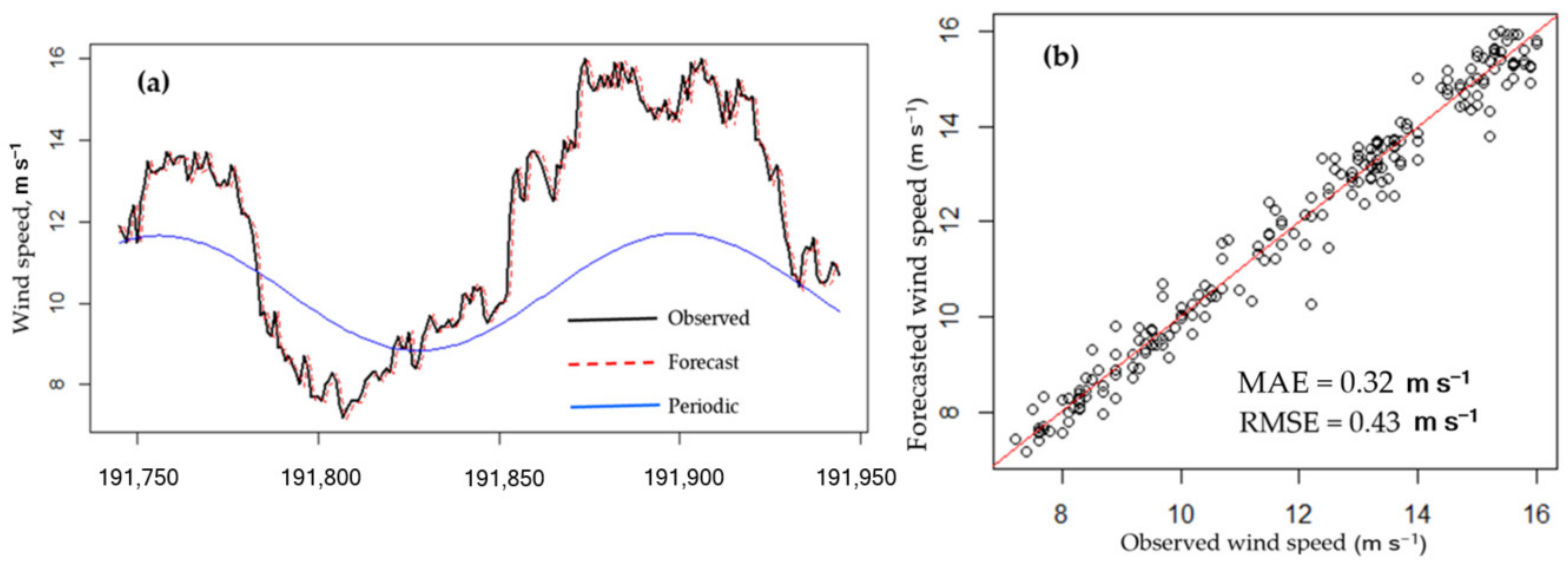
• The time series modeling, which takes into account the frequency domain and time domain characteristics, identified two periodic (annual and diurnal) components and a third-order autoregressive model for the multiple-year wind speed time series. An example was demonstrated that the proposed time series model yields good short period forecast results. The approach is general and can be applied to data series of other meteorological variables;
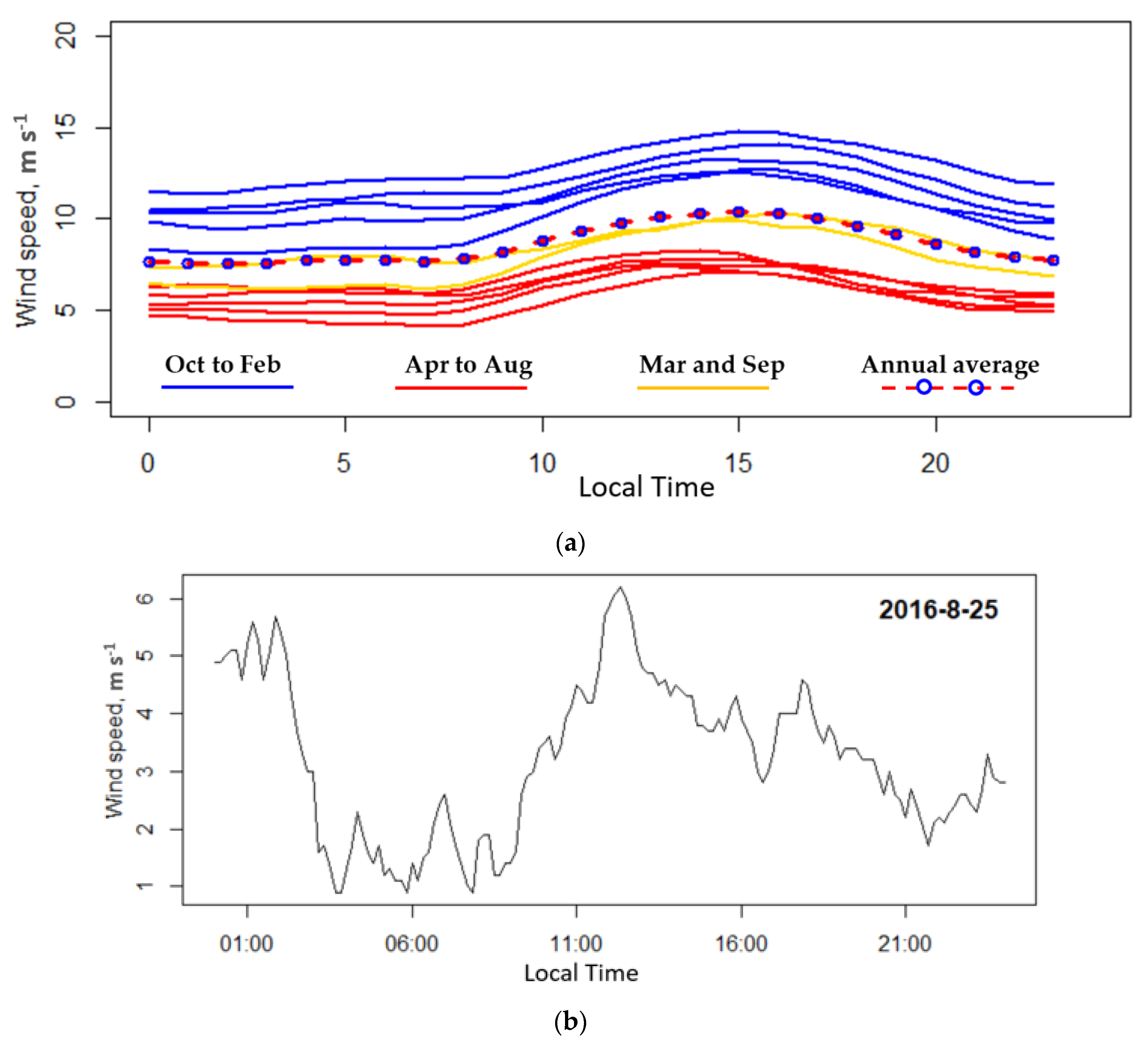
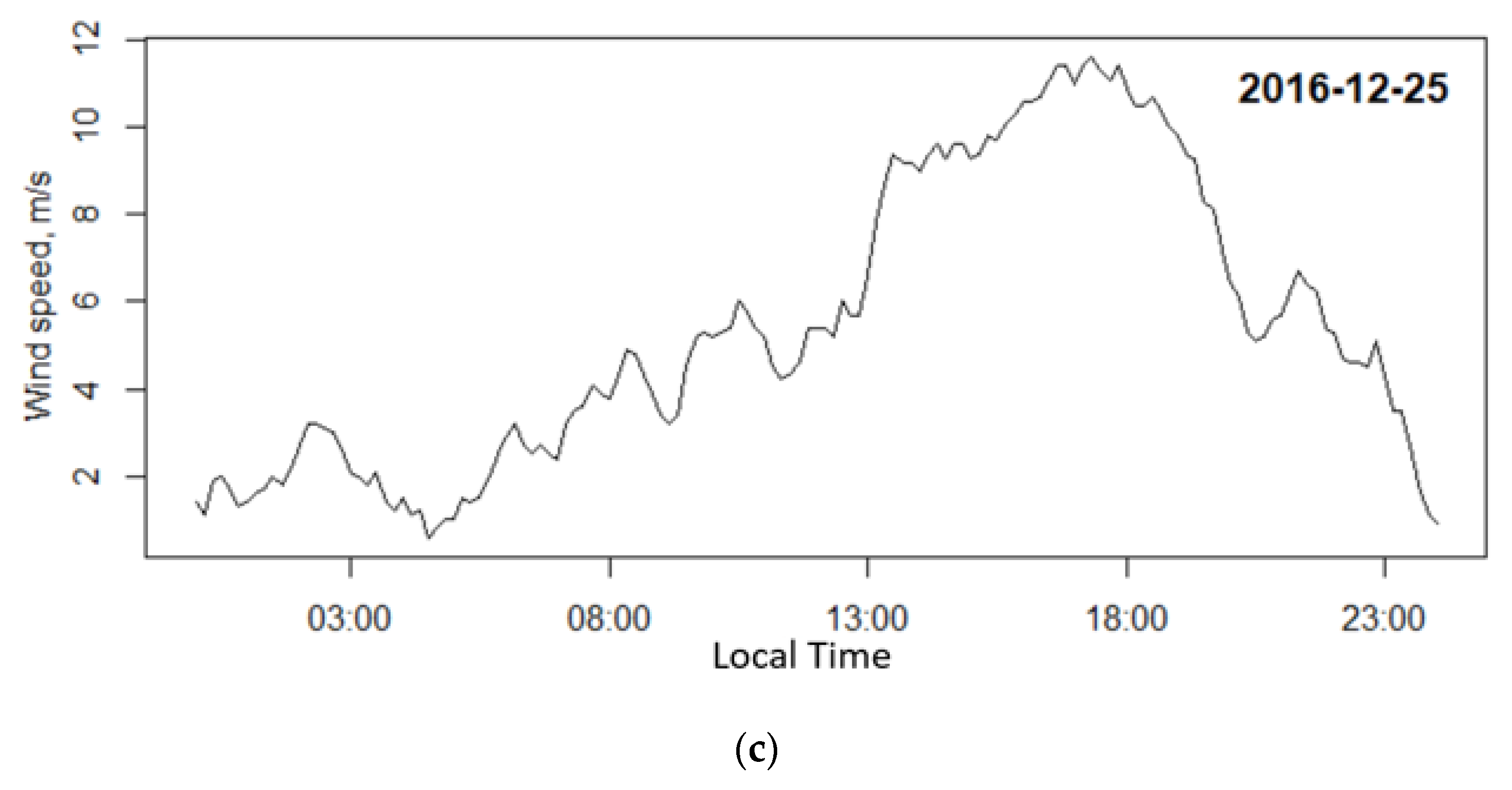
• There are distinct seasonal wind speed characteristics. Monthly-average wind speeds are high (>10 m s⁻¹) in mid-autumn to winter (October to February) and low (<7 m s⁻¹) in mid-spring to summer (April to August), with March and September being the transition period. Such seasonal characteristics explain the annual periodic component identified by the spectral analysis;
• The diurnal variation pattern also varies with months. The hours of peak occurrence of the high wind-speed months (October to February) are about 2 to 3 h later than that of the low wind-speed months (April to August), which is coincident with the situations caused by divergent zone and convergent zone related to sea breeze types. The time lag in the hours of peak occurrence of the high and low wind-speed seasons confirms that the sea breeze plays an important role in the magnitude of the wind speed;
• A new EACH method for sea breeze type identification is proposed in this study. The method converts the daily wind speed diagram into a constant average velocity vector which represents the effect of synoptic-scale weather system, and an ellipse which represents the effect of volatile regional weather system. The proposed method was further verified using the surface weather chart and lidar observation data;
• The proposed EACH method has the advantages of being scalable, adaptive, and easily programmable for an automated sea breeze type identification. It is also computationally efficient since only a few filtered days of wind speed data need to be processed;
• The verification process can collect environmental variables such as temperature difference, wind speed, wind direction, air humidity, air pressure, cloud cover, sunshine time, and precipitation for:

  ◦

  Setting up the thresholds of environmental variables to perfect rules;

  ◦

  Finding reasons for dates with trend-changing velocity to foresee variations in sea breeze speed.

• A good approximation for the magnitude of sea breeze velocity makes comparisons of different sites and different times easy;

In the near future, we hope

• A hybrid model consisting of the third-order autoregressive model and numerical weather prediction model can be developed to predict the occurrence of extreme events more accurately;
• To analyze more offshore wind speed data of central Taiwan to further validate the EACH method and obtain more insights into offshore behaviors of sea breezes in order to harness offshore wind energy.

References

- Offshore Wind-Power Generation. 13 June 2019. Available online: https://english.ey.gov.tw/News3/9E5540D592A5FECD/34ff3d6b-412e-458d-afe9-01737d2da52d (accessed on 1 November 2020).
- MOEA Plans a New Target to Develop Further 10 GW of Offshore Wind Capacity between 2026 to 2035-Anticipation of a Price Drop below the Average Consumer Price. 6 January 2020. Available online: https://www.moeaboe.gov.tw/ECW/english/news/News.aspx?kind=6&menu_id=958&news_id=16566 (accessed on 1 November 2020).
- Cheng, K.-S.; Ho, C.-Y.; Teng, J.-H. Wind Characteristics in the Taiwan Strait: A Case Study of the First Offshore Wind Farm in Taiwan. Energies 2020, 13, 6492. [Google Scholar] [CrossRef]
- Soman, S.S.; Zareipour, H.; Malik, O.; Mandal, P. A review of wind power and wind speed forecasting methods with different time horizons. In Proceedings of the North American Power Symposium 2010, Arlington, TX, USA, 26–28 September 2010. [Google Scholar]
- Milligan, M.; Schwartz, M.; Wan, Y.-h. Statistical Wind Power Forecasting Models: Results for US Wind Farms; National Renewable Energy Lab (NREL): Golden, CO, USA, 2003.
- Torres, J.L.; García, A.; De Blas, M.; De Francisco, A. Forecast of hourly average wind speed with ARMA models in Navarre (Spain). Sol. Energy 2005, 79, 65–77. [Google Scholar] [CrossRef]
- Gao, S.; He, Y.; Chen, H. Wind speed forecast for wind farms based on ARMA-ARCH model. In Proceedings of the 2009 International Conference on Sustainable Power Generation and Supply, Nanjing, China, 6–7 April 2009. [Google Scholar]
- Kavasseri, R.G.; Seetharaman, K. Day-ahead wind speed forecasting using f-ARIMA models. Renew. Energy 2009, 34, 1388–1393. [Google Scholar] [CrossRef]
- Rajagopalan, S.; Santoso, S. Wind power forecasting and error analysis using the autoregressive moving average modeling. In Proceedings of the 2009 IEEE Power & Energy Society General Meeting, Calgary, AB, Canada, 26–30 July 2009. [Google Scholar]
- Simpson, J.E. Sea Breeze and Local Winds; Cambridge University Press: Cambridge, MA, USA, 1994. [Google Scholar]
- Miller, S.T.K.; Keim, B.D.; Talbot, R.W.; Mao, H. Sea breeze: Structure, forecasting, and impacts. Rev. Geophys. 2003, 41, 124. [Google Scholar] [CrossRef] [Green Version]
- Steele, C.J.; Dorling, S.R.; von Glasow, R.; Bacon, J. Idealized WRF model sensitivity simulations of sea breeze types and their effects on offshore windfields. Atmos. Chem. Phys. 2013, 13, 443–461. [Google Scholar] [CrossRef] [Green Version]
- Steele, C.J.; Dorling, S.R.; von Glasow, R.; Bacon, J. Modelling sea-breeze climatologies and interactions on coasts in the southern North Sea: Implications for offshore wind energy. Q. J. R. Meteorol. Soc. 2015, 141, 1821–1835. [Google Scholar] [CrossRef] [Green Version]
- Borge, R.; Alexandrov, V.; Del Vas, J.J.; Lumbreras, J.; Rodríguez, E. A comprehensive sensitivity analysis of the WRF model for air quality applications over the Iberian Peninsula. Atmos. Environ. 2008, 42, 8560–8574. [Google Scholar] [CrossRef]
- Lee, S.-H.; Kim, S.-W.; Angevine, W.M.; Bianco, L.; McKeen, S.A.; Senff, C.J.; Trainer, M.; Tucker, S.C.; Zamora, R.J. Evaluation of urban surface parameterizations in the WRF model using measurements during the Texas Air Quality Study 2006 field campaign. Atmos. Chem. Phys. 2011, 11, 2127–2143. [Google Scholar] [CrossRef] [Green Version]
- Golding, B.; Clark, P.; May, B. The Boscastle flood: Meteorological analysis of the conditions leading to flooding on 16 August 2004. Weather 2005, 60, 230–235. [Google Scholar] [CrossRef]
- Crosman, E.T.; Horel, J.D. Sea and lake breezes: A review of numerical studies. Bound.-Layer Meteorol. 2010, 137, 1–29. [Google Scholar] [CrossRef] [Green Version]
- Liu, K.-Y.; Wang, Z.; Hsiao, L.-F. A modeling of the sea breeze and its impacts on ozone distribution in northern Taiwan. Environ. Model. Softw. 2002, 17, 21–27. [Google Scholar] [CrossRef]
- Lin, C.Y.; Chen, F.; Huang, J.C.; Chen, W.C.; Liou, Y.A.; Chen, W.N.; Liu, S.C. Urban heat island effect and its impact on boundary layer development and land–sea circulation over northern Taiwan. Atmos. Environ. 2008, 42, 5635–5649. [Google Scholar] [CrossRef]
- Yu, R.; Li, J.; Chen, H. Diurnal variation of surface wind over central eastern China. Clim. Dyn. 2009, 33, 1089–1097. [Google Scholar] [CrossRef]
- Shu, Z.R.; Li, Q.S.; Chan, P.W.; He, Y.C. Seasonal and diurnal variation of marine wind characteristics based on lidar measurements. Meteorol. Appl. 2020, 27, e1918. [Google Scholar] [CrossRef]
- Cook, N.J. A statistical model of the seasonal-diurnal wind climate at Adelaide. Aust. Meteorol. Oceanogr. J. 2015, 65, 206–232. [Google Scholar] [CrossRef]
- Yan, P.; Zuo, D.; Yang, P.; Li, S. Typical Modes of the Wind Speed Diurnal Variation in Beijing Based on the Clustering Method. Front. Phys. 2021, 9, 284. [Google Scholar] [CrossRef]
- Brown, B.G.; Katz, R.W.; Murphy, A.H. Time series models to simulate and forecast wind speed and wind power. J. Appl. Meteorol. Climatol. 1984, 23, 1184–1195. [Google Scholar] [CrossRef]
- Do, D.-P.N.; Lee, Y.; Choi, J. Hourly average wind speed simulation and forecast based on ARMA model in Jeju Island, Korea. J. Electr. Eng. Technol. 2016, 11, 1548–1555. [Google Scholar] [CrossRef] [Green Version]
- Huang, Z.; Chalabi, Z. Use of time-series analysis to model and forecast wind speed. J. Wind Eng. Ind. Aerodyn. 1995, 56, 311–322. [Google Scholar] [CrossRef]
- Haurwitz, B. Comments on the sea-breeze circulation. J. Atmos. Sci. 1947, 4, 1–8. [Google Scholar] [CrossRef] [Green Version]