Adaptive Smooth Variable Structure Filter Strategy for State Estimation of Electric Vehicle Batteries

Abstract

Battery Management Systems (BMSs) are used to manage the utilization of batteries and their operation in Electric and Hybrid Vehicles. It is imperative for efficient and safe operation of batteries to be able to accurately estimate the State of Charge (SoC), State of Health (SoH) and State of Power (SoP). The SoC and SoH estimation must remain robust and accurate despite aging and in presence of noise, uncertainties and sensor biases. This paper introduces a robust adaptive filter referred to as the Adaptive Smooth Variable Structure Filter with a time-varying Boundary Layer (ASVSF-VBL) for the estimation of the SoC and SoH in electrified vehicles. The internal model of the filter is a third-order equivalent circuit model (ECM) and its state vector is augmented to enable estimation of the internal resistance and current bias. It is shown that system and measurement noise covariance adaptation for the SVSF-VBL approach improves the performance in state estimation of a battery. The estimated internal resistance is then utilized to improve determination of the battery’s SoH. The effectiveness of the proposed method is validated using experimental data from tests on Lithium Polymer automotive batteries. The results indicate that the SoC estimation error can remain within less than $2\%$ over the full operating range of SoC along with an accurate estimation of SoH.

1. Introduction

Lithium-ion Batteries are extensively used for energy storage in Electric (EVs) and Hybrid Electric (HEVs) Vehicles due to their high energy and high power densities. The performance and efficiency of EVs and HEVs are largely affected by their Battery Management Systems (BMSs) that need to ensure a safe, stable and reliable operation for the battery pack. State of Charge (SoC), State of Health (SoH), and State of Power (SoP) are key operational parameters of the battery that need to be estimated and managed. These elements together provide a comprehensive view of the battery and the pack’s capabilities [1,2,3].

The battery SoC represents remaining charge in a battery which is similar to the gas-gauge in fossil-fuel vehicles. The SoC is a short-term indicator of the battery ability, however, it cannot provide valuable information about the health of the battery. The battery SoH is an indicator of the remaining battery capacity and life. The battery SoC and SoH need to be estimated as there are no sensors for their direct measurement. Accurate estimation of SoC and SoH are required to ensure an equal distribution of load among cells in the pack and to determine where a cell is in its life cycle. A wide range of strategies have been presented for both SoC and SoH estimation. The SoC estimation methods are categorized into direct and indirect methods [4,5].

Measurements of the terminal voltage, current and impedance are commonly employed in direct methods to calculate the battery SoC. Methods based on the open circuit voltage, terminal voltage, internal resistance and Coulomb Counting (CC) are commonly used. However, these methods require regular calibration due to error propagation related to changes in the internal characteristics of the battery due to aging, inaccuracies in the assumed initial conditions, and measurement biases [6]. Temperature and mechanical measurements of a cell have also been taken into consideration to improve the battery management and therefore states estimation [7]. However, indirect methods have been proven to be highly beneficial especially in uncertain conditions. Indirect methods include fuzzy logic-based estimation, artificial neural networks, and filter/observer-based techniques. Model-based strategies provide an insight into the internal dynamics of a battery and therefore could be more practical to use onboard of a BMS [8,9,10].

The battery SoH estimation has to take into account the battery capacity fade and impedance changes. SoH estimation methods are generally categorized into experimental or model-based techniques. Experimental-based techniques rely on characterization of batteries using cycling data. These methods involve measurement of internal resistance, impedance measurement, coulomb counting and regression analysis. Model-based strategies use filters and observers in conjunction with battery models to provide a real-time indicator for SoH estimation [11,12].

Battery models used in BMSs have included electrochemical and equivalent circuit models (ECMs). Electrochemical models are structured to represent the physical reactions inside a battery and therefore are suitable for degradation analysis. However, they have not been proven to be more accurate in SoC and SoH estimation and due to their complexity, are not commonly used onboard of a BMS. ECMs, on the other hand, provide a simple model which can be easily parameterized using experimental data, and provide sufficient accuracy for real-time parameter and state estimation. Additionally, in their modified forms provide thermal modeling or a measure of SoH [13]. For better accuracy, the parameters of ECMs require to be adjusted according to the battery’s SoH, temperature, and current (or C-rate). Different strategies have been reported for model adjustment including look-up tables as well as parameter estimation and multiple model strategies. Online parameter estimation is commonly considered to improve the performance by adapting the model for different conditions [14]. Multiple model strategies can also increase the adaptation of a battery by considering a range of scenarios [15,16]. Once a model is chosen to determine the dynamics of the battery, a robust filter is needed to estimate the states of the battery [17,18,19].

The Extended Kalman Filter (EKF) is the most commonly used filter for parameter estimation. Other methods include the Unscented KF (UKF), Quadrature KF (QKF), Sigma Point KF (SPKF), Cubature KF (CKF) and Particle Filter (PF) [20,21,22]. These strategies have been applied to lithium-ion batteries for state and parameter estimation [2,23,24,25]. Robust filtering strategies such as the Robust Kalman Filters, $H_{\infty }$ Filtering and the Smooth Variable Structure Filter (SVSF) have also been employed to deal with uncertainties [21,26,27]. In [28], SVSF with a Variable Boundary Layer (SVSF-VBL) is introduced to improve the performance of SVSF in presence of noise and uncertainties. More advancements on SVSF strategy have also been presented to boost the efficiency of the SVSF including the second-order SVSF, square-root SVSF, its combination with different filters such as KF, EKF, UKF, CKF, PF and more [29,30,31]. Although these methods enhance the accuracy of state estimation, they do not consider adaptability. Additionally, these algorithms can only be employed if the system is observable [32].

In the above filters, knowledge of the system’s model is an essential requirement for reliable state and parameter estimation. Characterization of noise statistics is needed as well as the dynamic model and affect the filter’s stability and performance. When this information is not correct, the performance of the designed filter may worsen significantly and could lead to divergence. Model-based filters such as the EKF assume that the system model is largely known together with the input functions and the noise statistics. However, this may not be the case in all applications and may need to be remedied through adaptive filters [33,34].

Two types of adaptation are considered in this paper, including filter tuning and multiple model (MM) methods. MM methods consider switching between a finite number of models to provide adaptability against changes and uncertainties. Different forms of multiple model methods have been proposed for state and parameter estimation of batteries [15,16,35]. Filter tuning methods, on the other hands, are used to adjust filter and model parameters as the system changes. Filter tuning methods can be categorized into noise adaptation, parameter tuning and joint filtering of parameters and states. Dual and joint estimation methods have been proposed in recent research for estimating both parameters and states of a battery simultaneously [36,37].

Noise statistics need to be captured for model-based filters. However, most filters usually assume that the noise is white, Gaussian and zero mean. If this assumption is not satisfied, the filter performance degrades. This has generated a great deal of interest in noise adjustments in a variety of applications. A wide range of studies have been performed concerning the properties, advantages, and disadvantages of different methods. In [38] different approaches for noise adaptations have been proposed for a KF. In [39], the maximum likelihood method is used in an adaptive KF (AKF) for an INS/GPS integration algorithm. A comparison of different strategies for noise covariance adaptation is presented in [40]. In [41], noise covariance adaptation is employed to a KF. Zhang proposed an adaptive KF for joint polarization tracking [34]. In [42], a comparison between different adaptive strategies for EKF is presented. In [43], sufficient conditions for noise covariance identification of a KF have been introduced.

Noise covariance estimation techniques can be broadly divided into two groups including feedback methods and feedback-free methods [40]. Simultaneous estimation of the states as well as the noise covariance matrices is performed in feedback methods. These methods include the covariance matching and the Bayesian methods. For feedback-free methods, on the other hand, estimated noise covariances are not required for state estimation. Examples are the correlation and the maximum-likelihood methods [38,40].

In battery states estimation, the current supplied by the battery and the terminal voltage are measured. Measurement uncertainties include sensor noise, drift, and bias. The disturbances in current and voltage sensors affect the performance of a BMS, so they need to be taken into account. Adaptive methods boost the performance of the estimation methods in presence of noise, sensor drift and bias. However, sensor drift and bias should still be identified, as well as noise, for calibration purposes and to ensure an efficient and safe operation [17]. Different strategies are employed for sensor calibration which often require operation of specific instruments irregularly. Online estimation of sensor bias is a widely used technique in real-time applications. In [32], the observability of a battery model is investigated in the presence of sensor bias. The effect of sensor bias and drift estimation on SoC estimation is considered in [17].

This work considers adaptation for both sensor bias as well as modeling uncertainties. An adaptive SVSF-VBL based strategy is proposed to reduce state estimation errors of a battery. The contributions of this paper are as follows:

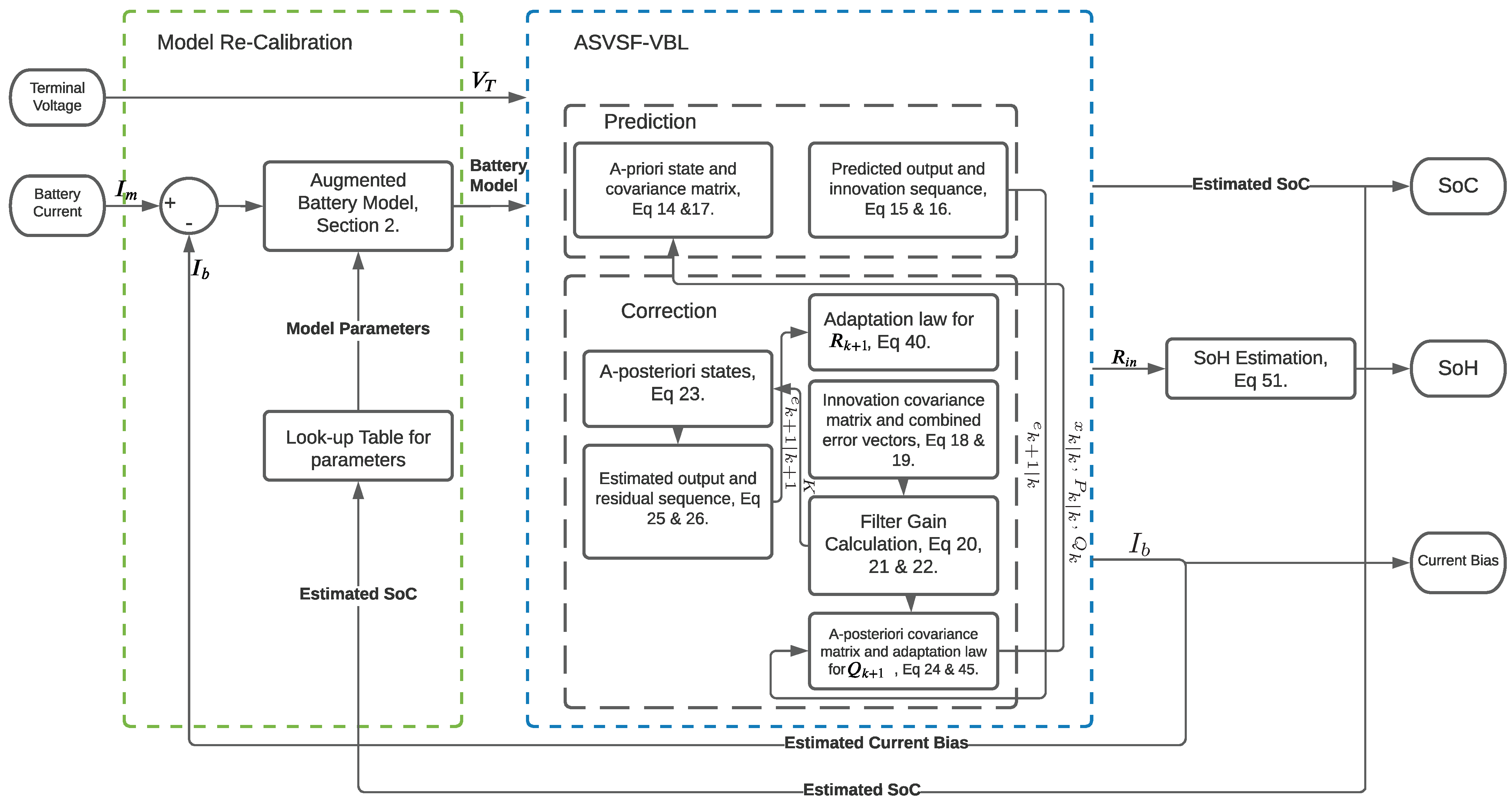
• An equivalent circuit model formulation augmented with internal resistance and sensor bias is used as the model. The estimated internal resistance is employed as an indicator of SoH while the estimated bias is to improve estimation accuracy.
• The Adaptive Smooth Variable Structure Filter with Variable Boundary Layer (ASVSF-VBL) strategy is introduced for state estimation (SoC and SoH) in presence of changing statics of noise and uncertainties. The proposed strategy provides noise adaptation which improves estimation robustness and accuracy.
• The performance of the ASVSF-VBL is then compared to conventional SVSF-VBL and EKF using experimental data.

Section 2 of this paper presents the model of the battery. The proposed ASVSF-VBL estimation strategy is introduced in Section 3. In Section 4, the proposed method is tested and validated using experimental data and its performance is comparatively analyzed. Section 5 concludes the paper.

2. Modeling

Equivalent Circuit Model (ECM) provides a simple and effective approach for battery characterization. Although, higher order models can be used to improve the battery model’s performance, a trade-off between complexity and accuracy should be considered to avoid over-parametrization that could affect estimation of the internal resistance. This study employs a third-order ECM to provide enough accuracy for a battery model especially when the battery ages while retaining the influence of aging on the internal resistance. Figure 1 shows a circuit diagram of a third-order ECM. The model contains different elements including a series resistance defined as internal resistance ($R_{in}$) and the Open Circuit Voltage (OCV) of the battery which relates to its SoC. The battery model also has multiple Resistance-Capacitance (RC) branches that describe the transients of the battery including the diffusion, the solid electrolyte interface (SEI) dynamics and the charge transfer kinetics. The structure of the model should reflects the dynamic complexity of the battery as it ages [44].

The battery model in Figure 1 is formulated with discrete-time state equations as follows,

$$\begin{array}{cc}\hfill & V_{1,k+1}=(1-\frac{\Delta T}{R_1{C}_1})V_{1,k}+\frac{\Delta T}{C_1}{i}_k,\hfill \\ \hfill & V_{2,k+1}=(1-\frac{\Delta T}{R_2{C}_2})V_{2,k}+\frac{\Delta T}{C_2}{i}_k,\hfill \\ \hfill & V_{3,k+1}=(1-\frac{\Delta T}{R_3{C}_3})V_{3,k}+\frac{\Delta T}{C_3}{i}_k,\hfill \\ \hfill & {SOC}_{k+1}={SOC}_k-\frac{\eta \Delta T}{C_n}{i}_k\hfill \end{array}$$

(1)

where $V_j,j=1,2,3$ are voltage across the RC branches, $C_j,j=1,2,3$ are capacitor and $R_j,j=1,2,3$ are resistance of the RC branches, i is the actual current flowing across the cell, $C_n$ is nominal capacity of the battery, $\eta$ is the cell Coulombic Efficiency, $\Delta T$ is the sampling period, and k is a time sample.

The output of the model is terminal voltage of the battery and is described as,

$$\begin{array}{cc}\hfill & V_{T,k}=V_{ocv}\left(SO{C}_k\right)-V_{1,k}-V_{2,k}-V_{3,k}-R_{in}{i}_k\hfill \end{array}$$

(2)

where $V_T$ is the cell terminal voltage, $V_{ocv}$ is the open circuit voltage (nonlinear function of SoC), and $R_{in}$ is the cell internal resistance.

The parameters of the model change with SoC and temperature. Therefore, parameters are constant within a small range of SoC, temperature and current level [45]. Updates of the model parameters or possibly its structure are needed for determining the battery SoH. The model can be modified using two approaches including model switching or parameter updating or estimation [15,46]. Parameter estimation can be employed if observability condition is satisfied. Here, the internal resistance is considered as a state that indicates the battery SoH and power capability [47].

$$\begin{array}{cc}\hfill & R_{in,k+1}=R_{in,k}+w_{r_k}\hfill \end{array}$$

(3)

where $w_{r_k}$ is white noise.

A bias may exist in the measured current of the battery due to sensor error [17,32]. Here, the current sensor bias is considered as an augmented state to the battery model to be estimated. This modification could optimize the estimation performance. The sensor bias is defined as follows,

$$\begin{array}{cc}\hfill & I_{b,k+1}=I_{b,k}+w_{b_k}\hfill \end{array}$$

(4)

where $i_b$ is the bias from the current sensor and $w_{b_k}$ is white noise. The measured current flowing across the cell ($i_m$) includes this bias and is defined as follows,

$$\begin{array}{cc}\hfill & I_{m,k}=I_k+I_{b,k}\hfill \end{array}$$

(5)

The modification is then applied to the model. Therefore, the state-space form of the proposed model is described as,

$$\begin{array}{cc}\hfill & x_{k+1}=f\left(x_k\right)+g\left(x_k\right)u_k,\hfill \end{array}$$

(6)

$$\begin{array}{cc}\hfill & y_k=h(x_k,u_k)\hfill \end{array}$$

(7)

where $x\in X$ is the state vector, $u\in \mathbb{R}$ is the input to the system, $y\in {\mathbb{R}}^m$ is the measurement vector, $f:X\to {\mathbb{R}}^n$ is the nonlinear system function, $g:X\to {\mathbb{R}}^n$ is the input gain and $h:X\to {\mathbb{R}}^m$ is the nonlinear measurement function where they are all differentiable functions. The state and measurement vectors are $x_k={\left[\begin{array}{cccccc}{V}_{1,k}& V_{2,k}& V_{3,k}& SO{C}_k& I_{b,k}& R_{in,k}\end{array}\right]}^{\mathrm{T}}$ and $y_k=V_{T,k}$, respectively. Note that in this model $f\left(x_k\right)$ is linear and $f\left(x_k\right)=A{x}_k$ and $g\left(x_k\right)=B$ are given as,

$$\begin{array}{cc}\hfill & A=\left[\begin{array}{cccccc}1-\frac{\Delta T}{R_1{C}_1}& 0& 0& 0& -\frac{\Delta T}{C_1}& 0\\ 0& 1-\frac{\Delta T}{R_2{C}_2}& 0& 0& -\frac{\Delta T}{C_2}& 0\\ 0& 0& 1-\frac{\Delta T}{R_3{C}_3}& 0& -\frac{\Delta T}{C_3}& 0\\ 0& 0& 0& 1& \frac{\eta \Delta T}{C_n}& 0\\ 0& 0& 0& 0& 1& 0\\ 0& 0& 0& 0& 0& 1\end{array}\right],B=\Delta T\left[\begin{array}{c}\frac{1}{C_1}\\ \frac{1}{C_2}\\ \frac{1}{C_3}\\ \frac{-\eta }{C_n}\\ 0\\ 0\end{array}\right]\hfill \end{array}$$

(8)

The output equation is a nonlinear function that can be specified as follows,

$$\begin{array}{cc}\hfill & V_{T,k}=V_{ocv}\left(SO{C}_k\right)-V_{1,k}-V_{2,k}-V_{3,k}+R_{in}{i}_{b,k}-R_{in}{i}_{m,k}\hfill \end{array}$$

(9)

The observability of this battery model can be guaranteed if $R_1{C}_1\ne R_2{C}_2\ne R_3{C}_3$ and there exists a $k\in \mathbb{Z}$ such that $\frac{\partial V_{ocv}^k}{\partial SO{C}^k}\ne 0$ [15]. Therefore, estimation strategies can be used here for state and parameter estimation.

3. Adaptive Smooth Variable Structure Filter with Variable Boundary Layer

The Adaptive Smooth Variable Structure Filter with Variable Boundary Layer (ASVSF-VBL) strategy is a method that adapt to the changes in the noise statistics. The approach improves the performance of the original SVSF-VBL and provides better accuracy and robustness in presence of noise and uncertainties. It is particularly applicable to battery SoC estimation as current bias is estimated and this increases the speed of noise statistic estimation. This section provides details on the proposed approach for state estimation.

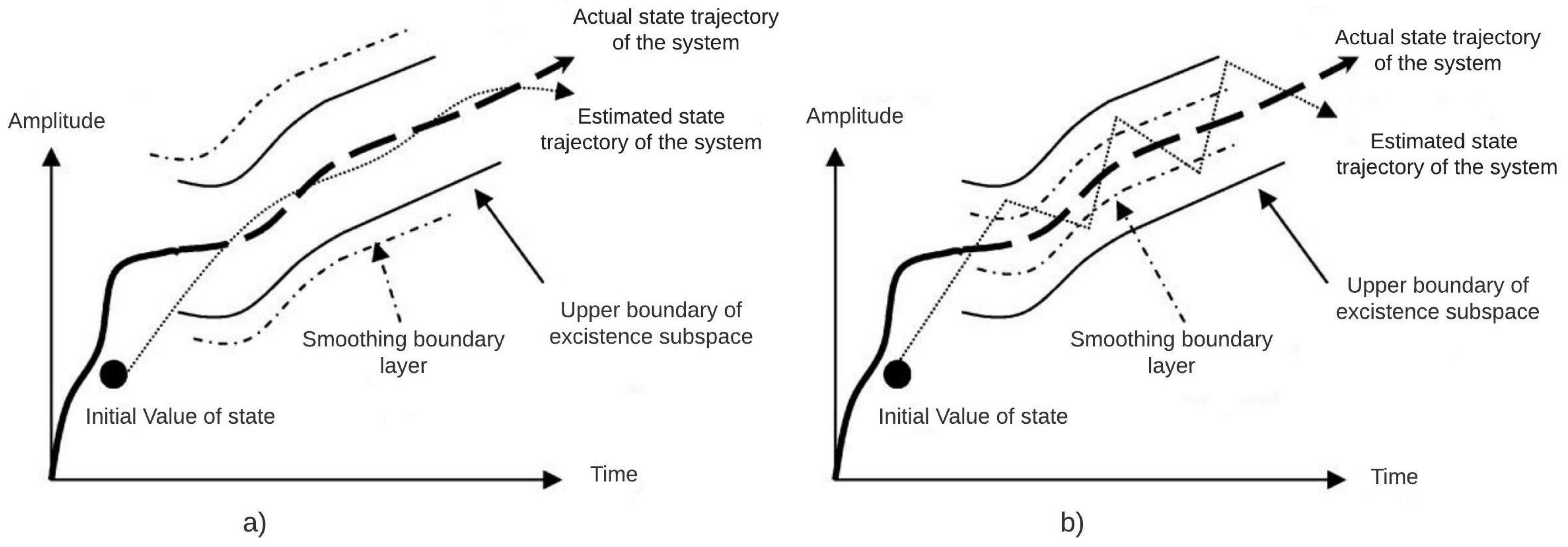
3.1. Smooth Variable Structure Filter with Variable Boundary Layer

The Variable Structure filter (VSF) approach was first presented in [26]. A revised version of it named SVSF was then introduced in [27] that is a predictor-corrector strategy based on the sliding mode concept. The method is applicable to linear and nonlinear systems with the assumption that the system under consideration is observable. The method provides stability and robustness to modeling uncertainties and noise with a given upper bound for the level of noise and unmodeled dynamics. Assuming a typical model is represented as follows,

$$\begin{array}{c}\hfill x_{k+1}=f(x_k,u_k,w_k),\end{array}$$

(10)

$$\begin{array}{c}\hfill z_k=h(x_k,u_k,{\upsilon }_k)\end{array}$$

(11)

where ${\upsilon }_k$ is the measurement noise and $w_k$ is the system noise and they are uncorrelated white noise with the following mean and covariance,

$$\begin{array}{cc}\hfill & E\left[w_k\right]=0,E\left[w_k{w}_k^T\right]=Q_k\hfill \end{array}$$

(12)

$$\begin{array}{cc}\hfill & E\left[{\upsilon }_k\right]=0,E\left[{\upsilon }_k{\upsilon }_k^T\right]=R_k\hfill \end{array}$$

(13)

The discontinuous corrective action of the SVSF method leads to chattering as shown in Figure 2. This chattering can be removed by using a smoothing boundary layer. The smoothing boundary layer will be inefficient if the disturbance exceeds the assumed upper bound [27]. A time-varying smoothing boundary layer eliminates chattering and excessive switching as presented in [48]. More advancement to the SVSF have also been proposed, including but not limited to covariance formulation, second-order SVSF, and combination of SVSF with other filters such as KF, EKF, UKF, PF, Square-Root SVSF and Two-pass SVSF [21,28,30,49]. The SVSF-VBL estimation is formulated as follows,

• Prediction: An estimated filter model is used to obtain the a-priori state estimates.

  $$\begin{array}{cc}\hfill & {\widehat{x}}_{k+1|k}=\widehat{A}{\widehat{x}}_{k|k}+\widehat{B}{u}_k,\hfill \end{array}$$

  (14)

  $$\begin{array}{cc}\hfill & {\widehat{z}}_{k+1|k}=\widehat{H}{\widehat{x}}_{k+1|k}\hfill \end{array}$$

  (15)

  $$\begin{array}{cc}\hfill & e_{k+1|k}=z_{k+1}-{\widehat{z}}_{k+1|k}\hfill \end{array}$$

  (16)

  $$\begin{array}{cc}\hfill & P_{k+1|k}=\widehat{A}{P}_{k|k}{\widehat{A}}^T+Q_k\hfill \end{array}$$

  (17)

  where P is the state vector covariance matrix, H is the jacobian matrix of H, and $e_{k+1|k}$ is called the filter innovation measurement sequence.
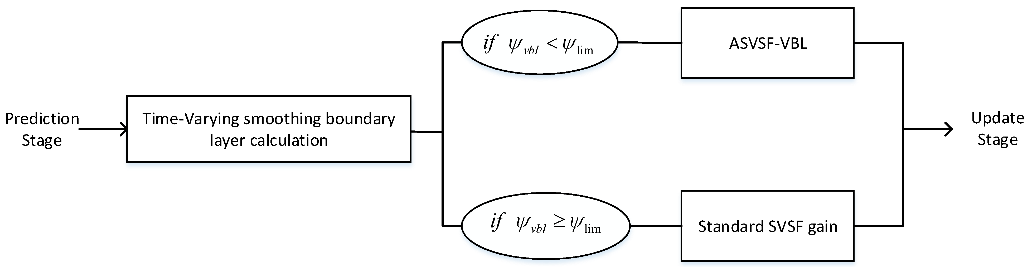
• Correction: The correction gain is obtained and, the estimated states are then updated from their a-priori into their a-posteriori by using this gain.

  $$\begin{array}{cc}\hfill & S_{k+1}=\widehat{H}{P}_{k+1|k}{\widehat{H}}^T+R_{k+1}\hfill \end{array}$$

  (18)

  $$\begin{array}{cc}\hfill & E_{k+1}=|e_{k+1|k}|+\gamma |e_{k|k}|\hfill \end{array}$$

  (19)

  $$\begin{array}{cc}\hfill & {\psi }_{k+1}={\left({\overline{E}}_{k+1}^{-1}\widehat{H}{P}_{k+1|k}{\widehat{H}}^T{S}_{k+1}^T\right)}^{-1}\hfill \end{array}$$

  (20)

  where S is the innovation covariance matrix, E is the combination of measurement error vector, $\gamma$ is the SVSF convergence parameter and ${\psi }_{k+1}$ is the SVSF smoothing boundary layer width.
  The SVSF is a predictor-corrector method and its gain is employed to update the a-priori estimated states. The gain ${\psi }_{k+1}<{\psi }_{lim}$ is as follows,

  $$\begin{array}{cc}\hfill & K_{k+1}={\widehat{H}}^{-1}{\overline{E}}_{k+1}{\psi }_{k+1}^{-1}\hfill \end{array}$$

  (21)

  where ${\psi }_{lim}$ is upper limit for the boundary layer. For the case when ${\psi }_{k+1}⩾{\psi }_{lim}$ the SVSF gain is:

  $$\begin{array}{cc}\hfill & K_{k+1}={\widehat{H}}^{-1}{\overline{E}}_{k+1}sat\left(e_{k+1|k}{\psi }_{k+1}^{-1}\right){\overline{e}}_{k+1|k}^{-1}\hfill \end{array}$$

  (22)
  Finally, the a posteriori parameters are calculated as:

  $$\begin{array}{cc}\hfill & {\widehat{x}}_{k+1|k+1}={\widehat{x}}_{k+1|k}+K_{k+1}{e}_{k+1|k}\hfill \\ \hfill & P_{k+1|k+1}=(I-K_{k+1}\widehat{H})P_{k+1|k}{(I-K_{k+1}\widehat{H})}^T\hfill \end{array}$$

  (23)

  $$\begin{array}{c}\hfill +K_{k+1}{R}_{k+1}{K}_{k+1}^T\end{array}$$

  (24)

  $$\begin{array}{cc}\hfill & {\widehat{z}}_{k+1|k+1}=\widehat{H}{\widehat{x}}_{k+1|k+1}\hfill \end{array}$$

  (25)

  $$\begin{array}{cc}\hfill & e_{k+1|k+1}=z_{k+1}-{\widehat{z}}_{k+1|k+1}\hfill \end{array}$$

  (26)

  where $e_{k+1|k+1}$ is called the filter measurement residual sequence. Equations (14) to (26) summarize the SVSF-VBL strategy.

3.2. Noise Adaptation for Smooth Variable Structure Filter

This paper proposes a novel form of SVSF-VBL that incorporates adaptation to noise statistics. Although the stability and estimation convergence of the SVSF-VBL method is proven with the time-varying boundary layer, its performance is significantly enhanced with adaptation to noise statistics variation and by including bias estimation in measurements. Figure 3 offers a brief overview of the ASVSF-VBL strategy that is explained on this section.

Different strategies have been proposed for noise adaptation including covariance matching, Bayesian, Maximum likelihood and correlation method. These methods have been tested in different applications to improve estimation performance. In the ASVSF-VBL, the system and measurement noise covariance matrices (Q and R) are adapted in time using the covariance matching method. The covariance matching technique employs the innovation and the residual defined in Equations (16) and (26) to adapt the estimated value of the system and measurement noise covariance matrices. Maximization of likelihood functions is used here to derive innovation-based adaptation for the measurement noise covariance matrix (R) using the SVSF-VBL method. The likelihood maximization estimation provides a unique and consistent value for measurement noise covariance matrix (R) estimation. The system noise covariance matrix (Q) is then estimated using the difference between a-posteriori and a-priori states. The optimization is performed in real-time for each time instant [41,42,43,50]. The assumptions for the ASVSF-VBL are as follows,

• The states are independent of the adaptive parameters.
• The system and measurement matrices are time variant within a piece-wise limit and independent of adaptive parameters.
• The innovation sequence is white and ergodic within the estimation window.

For Gaussian distribution, the probability density function of the measurements conditioned on an adaptive parameter at a specific epoch of $k+1$ is defined as,

$$\begin{array}{c}\hfill P{\left(z\right|\alpha )}_{k+1}=\frac{1}{\sqrt{{\left(2\pi \right)}^m\left|C_{{ϵ}_{k+1}}\right|}}{e}^{-\frac{1}{2}{ϵ}_{k+1}^T{C}_{{ϵ}_{k+1}}^{-1}{ϵ}_{k+1}}\end{array}$$

(27)

where ${ϵ}_{k+1}=z_{k+1}-z_{k+1|k}$ is the innovation sequence, $C_{v_{k+1}}$ is the innovation sequence covariance matrix, m is the number of measurements, and $\alpha$ is the adaptive parameter. The $z_{k+1|k}$ is obtained from Equation (15). The logarithmic form of the above equation is

$$\begin{array}{cc}\hfill & ln\left(P{\left(z\right|\alpha )}_{k+1}\right)=-\frac{1}{2}\{mln\left(2\pi \right)+ln\left(\right|C_{{ϵ}_{k+1}}\left|\right)+ln({ϵ}_{k+1}^T{C}_{{ϵ}_{k+1}}^{-1}{ϵ}_{k+1})\}\hfill \end{array}$$

(28)

For a fixed-length memory filter, the innovation matrix will only be considered inside a window of size N. Therefore, the ML optimization problem is defined as follows,

$$\begin{array}{c}\hfill \begin{array}{cc}\hfill \underset{\alpha }{min}& \sum _{i=i_0}^{k+1}ln|C_{{ϵ}_i}|+\sum _{i=i_0}^{k+1}({ϵ}_i^T{C}_{{ϵ}_i}^{-1}{ϵ}_i)\hfill \end{array}\end{array}$$

(29)

where $i_0=k-N+2$ is the first epoch inside the estimation. The above formula defines the best estimate as it has the maximum likelihood based on the adaptive parameters. This optimization problem can be simplified using matrix differential calculus as,

$$\begin{array}{cc}\hfill & \sum _{i=i_0}^{k+1}\left[tr\left\{C_{{ϵ}_i}^{-1}\frac{\partial C_{{ϵ}_i}}{\partial {\alpha }_{k+1}}\right\}-{ϵ}_i^T{C}_{{ϵ}_i}^{-1}\frac{\partial C_{{ϵ}_i}}{\partial {\alpha }_{k+1}}{C}_{{ϵ}_i}^{-1}{ϵ}_i\right]=0\hfill \end{array}$$

(30)

The partial derivative of Equation (18) with respect to $\alpha$ is,

$$\begin{array}{cc}\hfill & \frac{\partial C_{{ϵ}_k}}{\partial {\alpha }_{k+1}}=\frac{\partial R_{k+1}}{\partial {\alpha }_{k+1}}+H\frac{\partial P_{k+1|k}}{\partial {\alpha }_{k+1}}{H}^T\hfill \end{array}$$

(31)

And taking partial derivative from Equation (17) with respect to $\alpha$ gives,

$$\begin{array}{cc}\hfill & \frac{\partial P_{k+1|k}}{\partial {\alpha }_{k+1}}=A\frac{\partial P_{k|k}}{\partial {\alpha }_{k+1}}{A}^T+\frac{\partial Q_k}{\partial {\alpha }_{k+1}}\hfill \end{array}$$

(32)

Assuming that the process inside the estimation window is in steady state, Equation (32) can be written as,

$$\begin{array}{cc}\hfill & \frac{\partial P_{k+1|k}}{\partial {\alpha }_{k+1}}=\frac{\partial Q_k}{\partial {\alpha }_{k+1}}\hfill \end{array}$$

(33)

By substituting Equation (33) into (31) and applying it into (30) the maximum likelihood equation for the adaptive SVSF-VBL is as follows,

$$\begin{array}{cc}\hfill & \sum _{i=i_0}^{k+1}tr\left\{\left[C_{{ϵ}_i}^{-1}-C_{{ϵ}_i}^{-1}{ϵ}_i{ϵ}_i^T{C}_{{ϵ}_i}^{-1}\right]\left[\frac{\partial R_i}{\partial {\alpha }_{k+1}}+H\frac{\partial Q_{i-1}}{\partial {\alpha }_{k+1}}{H}^T\right]\right\}=0\hfill \end{array}$$

(34)

Both system and measurement noise covariance matrices (Q and R) can be adapted based on $\alpha$ from the computed equation. To achieve an expression for R, ${\alpha }_{ii}=R_{ii}$ is considered where the adaptive parameters are the variance of the updated measurement. Therefore, Equation (34) is modified as follows,

$$\begin{array}{cc}\hfill & \sum _{i=i_0}^{k+1}tr\left\{C_{{ϵ}_i}^{-1}\left[C_{{ϵ}_i}-{ϵ}_i{ϵ}_i^T\right]C_{{ϵ}_i}^{-1}\right\}=0\hfill \end{array}$$

(35)

This equation is solved by defining the innovation sequence as,

$$\begin{array}{cc}\hfill & C_{{ϵ}_{k+1}}=\frac{1}{N}\sum _{i=i_0}^{k+1}{ϵ}_i{ϵ}_i^T\hfill \end{array}$$

(36)

Replacing Equation (36) into (18),

$$\begin{array}{cc}\hfill & R_{k+1}=C_{{ϵ}_{k+1}}-\widehat{H}{P}_{k+1|k}{\widehat{H}}^T\hfill \end{array}$$

(37)

Since the measurement noise covariance should be positive definite, a more stable expression is required. For the case with ${\psi }_{k+1}<{\psi }_{lim}$, it can be shown that the adaptation rule for R is,

$$\begin{array}{cc}\hfill & R_{k+1}={\widehat{C}}_{{\epsilon }_{k+1}}+\widehat{H}{P}_{k+1|k+1}{\widehat{H}}^T\hfill \end{array}$$

(38)

where the residual sequence is $\epsilon =z_{k+1}-z_{k+1|k+1}$ and residual covariance matrix ${\widehat{C}}_{{\epsilon }_{k+1}}$ can be calculated as,

$$\begin{array}{cc}\hfill & {\widehat{C}}_{{\epsilon }_{k+1}}=\frac{1}{N}\sum _{i=i_0}^{k+1}{\epsilon }_i{\epsilon }_i^T\hfill \end{array}$$

(39)

A forgetting factor is then employed to provide a smoother estimation of R,

$$\begin{array}{c}\hfill R_{k+1}={\lambda }_R{R}_k+(1-{\lambda }_R)({\widehat{C}}_{{\epsilon }_{k+1}}+\widehat{H}{P}_{k+1|k+1}{\widehat{H}}^T)\end{array}$$

(40)

where $0\le {\lambda }_R\le 1$.

The process noise covariance (Q) can be achieved using the SVSF-VBL formulation. Considering the system Equation (10) as,

$$\begin{array}{cc}\hfill & w_k=x_{k+1}-f(x_k,uk)\hfill \end{array}$$

(41)

From Equations (41) and (14), the estimated system noise can be obtained as,

$$\begin{array}{cc}\hfill & {\widehat{w}}_k=x_{k+1|k+1}-f(x_{k|k},uk)=x_{k+1|k+1}-x_{k+1|k}=K{e}_{k+1|k}\hfill \end{array}$$

(42)

Covariance of ${\widehat{w}}_k$ can be written as,

$$\begin{array}{cc}\hfill & E\left[{\widehat{w}}_k{{\widehat{w}}_k}^T\right]=E\left[K{e}_{k+1|k}{\left[K{e}_{k+1|k}\right]}^T\right]=K{C}_{{ϵ}_{k+1}}{K}^T\hfill \end{array}$$

(43)

$$\begin{array}{cc}\hfill & Q_k=K{C}_{{ϵ}_{k+1}}{K}^T\hfill \end{array}$$

(44)

A forgetting factor is also considered for Q to update it gradually [41],

$$\begin{array}{c}\hfill Q_{k+1}={\lambda }_Q{Q}_k+(1-{\lambda }_Q)\left(K{\widehat{C}}_{k+1}{K}^T\right)\end{array}$$

(45)

where $0\le {\lambda }_R\le 1$.

Figure 4 illustrates an overview of the proposed ASVSF-VBL method specified for state estimation of electric vehicle batteries. The SVSF filter guarantees stability using a Lyapunov function. Based on Lyapunov theory, if a Lyapunov function (V) is locally positive definite and the time derivative of it is locally negative semi-definite, the filter is stable [27]. The following Lyapunov function is considered based on the a-posteriori estimation error (residual error),

$$\begin{array}{c}\hfill V=e_{k+1|k+1}^T{e}_{k+1|k+1}>0\end{array}$$

(46)

Therefore, the estimation process is stable if the following condition is satisfied,

$$\begin{array}{c}\hfill \Delta V⩽0\end{array}$$

(47)

where $\Delta V$ is defined as follows,

$$\begin{array}{c}\hfill \Delta V=e_{k+1|k+1}^T{e}_{k+1|k+1}-e_{k+1|k}^T{e}_{k+1|k}\end{array}$$

(48)

Therefore, the following condition which is equal to Equation (46) satisfies the stability condition of the estimation process [27].

$$\begin{array}{c}\hfill {|e_{k|k}|}_{Abs}>{|e_{k+1|k+1}|}_{Abs}\end{array}$$

(49)

Theorem 1

([27]). On the stability of the SVSF strategy, if the system is stable, consecutive bijective (or completely observable and completely controllable in the case of linear systems), then the SVSF corrective gain $K_{k+1}$ that would satisfy the stability condition of (49) is subject to the following conditions,

$$\begin{array}{c}\hfill {|e_{k+1|k}|}_{Abs}⩽{|K_{k+1}|}_{Abs}<{|e_{k+1|k}|}_{Abs}+{|e_{k|k}|}_{Abs}\end{array}$$

(50)

The corrective gain $K_{k+1}$ of the SVSF as Equation (22) satisfies this condition [27]. The SVSF gain is not affected by the adaptive scheme outside the boundary layer and hence BIBO stability of the ASVSF-VBL remains unaffected.

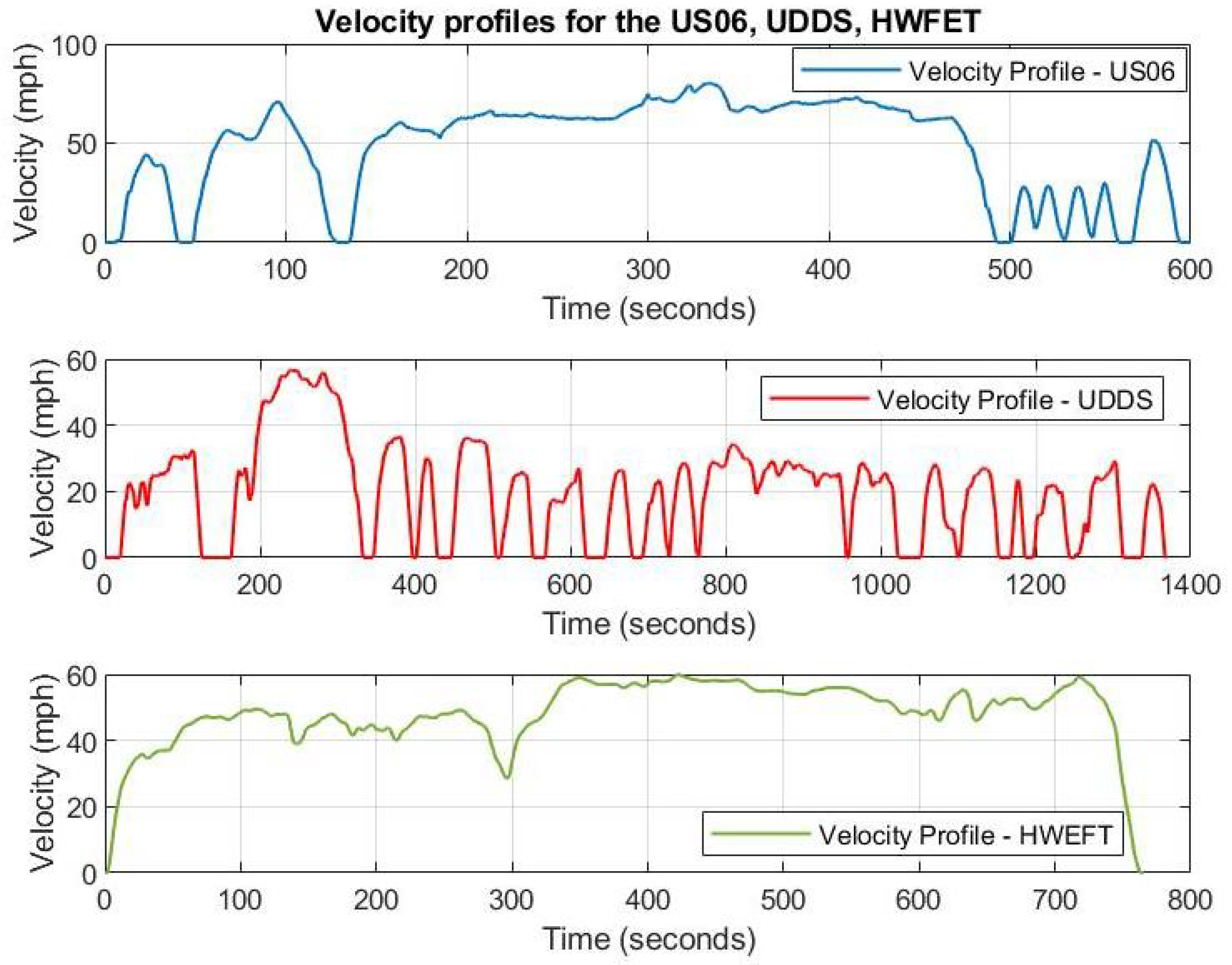
4. Experimental Results

The ASVSF-VBL was validated and comparatively studied further to experiments conducted on NMC Lithium Polymer battery cells. Battery cells specifications are presented in

Table 1. Battery cells specifications.

Manufacture	Batterist
Type	NMC Li-ion Polymer
Nominal Capacity (mAh)	5400
Nominal Voltage (V)	3.7
Minimum Voltage (V)	2.8
Maximum Voltage (V)	4.2

. The experiments were conducted by using an experimental setup consisting of an Arbin BT2000 cycler, environmental chambers, an AVL Lynx data acquisition system, and AVL Lynx software [45]. The characterization tests included static capacity, internal resistance, OCV-SOC and efficiency tests; these were conducted to obtain a baseline for the battery cell performance. In addition, cycling tests were done to investigate the impact of aging on the battery’s performance and dynamics.

Different driving cycles including an Urban Dynamometer Driving Schedule (UDDS); a light duty drive cycle for high speed and high load (US06); and, a High Fuel Economy Test (HWFET) drive cycle were used in this study. Figure 5 presents the standard driving cycles considered in this article. These drive cycles simulate common driving patterns. The driving patterns of an average driver in the city are illustrated in Figure 5 and were assumed to be the UDDS cycle. High acceleration driving conditions with aggressive driving patterns are performed by US06 drive cycle. The HWFET drive cycle represents highway driving. A mixture of these velocity profiles was used to generate a current profile for the battery cell as presented in Figure 6. The experimental data was collected for battery cells over time at elevated temperatures ranging from ${35}^{\circ }$ to ${40}^{\circ }$ to accelerate aging for a full range of SoCs from $90\%$ to $20\%$ [1,45].

The battery model should be determined as an essential part of estimation. Battery model parameters are first identified for different levels of SoC (Figure 6) as well as SoH [45].

Table 2. Model Parameters bound of a third-order ECM. Example given for $80\%$ SoC and $100\%$ SOH.

Parameters	${\mathit{R}}_1\left(\mathbf{\Omega }\right)$	${\mathit{R}}_2\left(\mathbf{\Omega }\right)$	${\mathit{R}}_3\left(\mathbf{\Omega }\right)$	${\mathit{\tau }}_1\left(\mathbf{s}\right)$	${\mathit{\tau }}_2\left(\mathbf{s}\right)$	${\mathit{\tau }}_3\left(\mathbf{s}\right)$
Upper Bound	0.025	0.0079	0.089	1	27	355
Lower Bound	0.00117	0.000038	0.0012	0.1	8	74
Example	0.0018	0.0028	0.0082	0.5543	11.929	111.57

provides the parametric bound of the equivalent circuit model presented in Section 2. The internal resistance of the battery is considered as a parameter to be estimated in real time. The internal resistance is one of the key factors for determining the battery’s SoH and reflects the power capability of a battery. The battery’s SoH is estimated using an indicator as follows,

$$\begin{array}{c}\hfill {SOH}_R=\frac{R_{EOL}-R_{in}}{R_{EOL}-R_{new}}\times 100\%\end{array}$$

(51)

where $R_{EOL}$ is the internal resistance of a fully aged battery, $R_{new}$ is the internal resistance of a fresh battery where it can be estimated based on experimental characterization or obtained from manufacturer’s specifications. The $R_{in}$ is the estimated internal resistance provided by the ASVSF-VBL strategy. The end of life for a battery in electric applications is usually where the nominal capacity is about $80\%$ compared to its value when the battery is new. Equation (51) indicates a value in range of $0⩽{SoH}_R⩽1$ which means that the battery reached its end of life and should be replaced. The presented value should be redefined in the range of $0.8⩽So{H}_R⩽1$ which means that $C_{n,old}=0.8C_{n,new}$ [12,52].

The ASVSF-VBL strategy as illustrated in Figure 4 is then employed to estimates the states of a battery including the internal resistance, the SoC and the current bias. Figure 7 demonstrates the validation data used to investigate the performance of the proposed method. Data was collected during experiments for a smaller range of SoC based on a US06 drive cycle for validation. Through the validation cycle, the battery cell’s voltage is measured and recorded as fast as 10 Hz. These measurements are then employed to evaluate the proposed strategy. A comparison of the ASVSF-VBL versus the SVSF-VBL and the EKF methods is provided to investigate the performance of the proposed strategy under different conditions. All filters use the same models with the same initial parameters for providing a direct comparison between the performance of the three filters. Optimal and non-optimal initial parameters are considered to show the effect of Q and R on the filters as listed in

Table 3. Initial parameters used for the filters.

Parameters	R	Q	P	${\mathit{I}}_{\mathit{b}0}$	$\mathit{\psi }$	$\mathit{\gamma }$
Optimal Value	5	$0.1I_6$	$I_6$	0	6	0.23
Non-Optimal Value	50	$I_6$	$I_6$	1	6	0.23

. In a non-ideal scenario a current bias of $I_b=1A$ has been added to the current measurement. In addition, extra noise has been added to measurements to simulate changing statistics of noise under controlled conditions.

Table 4. Root mean square errors of ASVSF-VBL in comparison with SVSF-VBL and EKF for different scenarios.

Different Scenarios		Ideal Scenario		In Presence of Noise and Current Bias
Initial Conditions		Optimal Initial Noise Covariance	Non-Optimal Initial Noise Covariance	Optimal Initial Noise Covariance	Non-Optimal Initial Noise Covariance
${RMSE}_{SOC}$	EKF	1.9735	0.5033	1.2640	2.5416
	SVSF-VBL	0.3776	0.3776	0.5207	0.6462
	ASVSF-VBL	0.4304	0.4304	0.5386	0.5386
${RMSE}_{V_t}$	EKF	0.000499	0.000695	0.0005477	0.000441
	SVSF-VBL	0.000276	0.000276	0.000241	0.000241
	ASVSF-VBL	0.00014	0.00014	0.00032	0.00032

provides the root mean square error of the results for two different scenarios. Firstly, an ideal scenario is considered where there are no added measurement bias and noise. Secondly, the filters have been tested in the presence of added noise and bias to the measurements. The results indicate that the proposed method using ASVSF-VBL provides a more accurate performance especially in the presence of added noise and bias disturbances. To illustrate the sensitivity of other methods to unknown noise statistics, Q and R are incorrectly specified as in Table 3. Figure 8a,b show the estimated SoC for both scenarios. The actual SoCs in these figures are evaluated using coulomb counting method from the cycler’s data. This is because the initial value of SoC and nominal capacity of a battery are both known during a laboratory experiment. It can be seen from Figure 8b that after 1500 s the EKF error increases when the drive cycle C-rate is high as illustrated in Figure 7. Figure 9a,b display the percentage of SoC estimation error for both scenarios. It can be observed that the proposed strategy can keep the percentage of SoC error to less than $2\%$. It is also shown in Figure 10 and Figure 11 that the proposed strategy is superior in identifying the current bias and internal resistance compared to the EKF and SVSF-VBL methods.

5. Conclusions

An adaptive strategy referred to as the Adaptive Smooth Variable Structure Filter with Variable Boundary Layer (ASVSF-VBL) is proposed to estimate the SoC and SoH of a battery. The ASVSF-VBL is model-based and, in this study, a third-order Equivalent Circuit Model (ECM) was used as the filter model. In addition to the SoC and SoH, the state vector was augmented to estimate the bias in current measurement and the battery’s internal resistance. The ASVSF-VBL adjusts the unknown system and measurement noise covariance matrices to provide a better performance under conditions involving noise with changing statistics. The adaptation scheme does not affect the stability of the estimation process. The estimated internal resistance of the ASVSF-VBL is used as an indicator of the battery SoH in addition to SoC. The proposed strategy was comparatively validated using experimental data and demonstrated a considerable improvement in performance. The proposed ASVSF-VBL reduced the estimated error of voltage to about 0.14 mV compared to the SVSF-VBL and EKF. The presented strategy showed the lowest SoC estimation error that remains within $2\%$ with an RMSE of approximately 0.4.

References

1. Ahmed, R.; El Sayed, M.; Arasaratnam, I.; Tjong, J.; Habibi, S. Reduced-order electrochemical model parameters identification and soc estimation for healthy and aged li-ion batteries part i: Parameterization model development for healthy batteries. IEEE J. Emerg. Sel. Top. Power Electron. 2014, 2, 659–677. [Google Scholar] [CrossRef]
2. Wang, Y.; Tian, J.; Sun, Z.; Wang, L.; Xu, R.; Li, M.; Chen, Z. A comprehensive review of battery modeling and state estimation approaches for advanced battery management systems. Renew. Sustain. Energy Rev. 2020, 131, 110015. [Google Scholar] [CrossRef]
3. Park, S.; Ahn, J.; Kang, T.; Park, S.; Kim, Y.; Cho, I.; Kim, J. Review of state-of-the-art battery state estimation technologies for battery management systems of stationary energy storage systems. J. Power Electron. 2020, 20, 1526–1540. [Google Scholar] [CrossRef]
4. Ahmed, R.; Sayed, M.E.; Arasaratnam, I.; Tjong, J.; Habibi, S. Reduced-Order Electrochemical Model Parameters Identification and State of Charge Estimation for Healthy and Aged Li-Ion Batteries—Part II: Aged Battery Model and State of Charge Estimation. IEEE J. Emerg. Sel. Top. Power Electron. 2014, 2, 678–690. [Google Scholar] [CrossRef]
5. Baccouche, I.; Jemmali, S.; Mlayah, A.; Manai, B.; Amara, N.E.B. Implementation of an Improved Coulomb-Counting Algorithm Based on a Piecewise SOC-OCV Relationship for SOC Estimation of Li-IonBattery. arXiv 2018, arXiv:1803.10654. [Google Scholar]
6. Movassagh, K.; Raihan, A.; Balasingam, B.; Pattipati, K. A critical look at Coulomb counting approach for state of charge estimation in batteries. Energies 2021, 14, 4074. [Google Scholar] [CrossRef]
7. Wei, Z.; Zhao, J.; He, H.; Ding, G.; Cui, H.; Liu, L. Future smart battery and management: Advanced sensing from external to embedded multi-dimensional measurement. J. Power Sources 2021, 489, 229462. [Google Scholar] [CrossRef]
8. Plett, G. Extended Kalman filtering for battery management systems of LiPB-based HEV battery packs-Part 1. Background. J. Power Sources 2004, 134, 252–261. [Google Scholar] [CrossRef]
9. Piller, S.; Perrin, M.; Jossen, A. Methods for state-of-charge determination and their applications. J. Power Sources 2001, 96, 113–120. [Google Scholar] [CrossRef]
10. Samadani, S.E.; Fraser, R.A.; Fowler, M. A Review Study of Methods for Lithium-Ion Battery Health Monitoring and Remaining Life Estimation in Hybrid Electric Vehicles; Technical Report, SAE Technical Paper; SAE International: Warrendale, PA, USA, 2012; Available online: https://www.sae.org/publications/technical-papers/content/2012-01-0125/ (accessed on 10 October 2021).
11. Berecibar, M.; Gandiaga, I.; Villarreal, I.; Omar, N.; Van Mierlo, J.; Van den Bossche, P. Critical review of state of health estimation methods of Li-ion batteries for real applications. Renew. Sustain. Energy Rev. 2016, 56, 572–587. [Google Scholar] [CrossRef]
12. Waag, W.; Fleischer, C.; Sauer, D.U. Critical review of the methods for monitoring of lithium-ion batteries in electric and hybrid vehicles. J. Power Sources 2014, 258, 321–339. [Google Scholar] [CrossRef]
13. Lin, X.; Perez, H.E.; Siegel, J.B.; Stefanopoulou, A.G. Robust estimation of battery system temperature distribution under sparse sensing and uncertainty. IEEE Trans. Control Syst. Technol. 2019, 28, 753–765. [Google Scholar] [CrossRef]
14. Wei, Z.; Zhao, J.; Xiong, R.; Dong, G.; Pou, J.; Tseng, K.J. Online estimation of power capacity with noise effect attenuation for lithium-ion battery. IEEE Trans. Ind. Electron. 2018, 66, 5724–5735. [Google Scholar] [CrossRef]
15. Rahimifard, S.; Ahmed, R.; Habibi, S. Interacting Multiple Model Strategy for Electric Vehicle Batteries State of Charge/Health/ Power Estimation. IEEE Access 2021, 9, 109875–109888. [Google Scholar] [CrossRef]
16. Messing, M.; Rahimifard, S.; Shoa, T.; Habibi, S. Low Temperature, Current Dependent Battery State Estimation Using Interacting Multiple Model Strategy. IEEE Access 2021, 9, 99876–99889. [Google Scholar] [CrossRef]
17. Lin, X. Theoretical analysis of battery SOC estimation errors under sensor bias and variance. IEEE Trans. Ind. Electron. 2018, 65, 7138–7148. [Google Scholar] [CrossRef]
18. Smiley, A.; Plett, G.L. An adaptive physics-based reduced-order model of an aged lithium-ion cell, selected using an interacting multiple-model Kalman filter. J. Energy Storage 2018, 19, 120–134. [Google Scholar] [CrossRef]
19. Farag, M.; Fleckenstein, M.; Habibi, S. Continuous piecewise-linear, reduced-order electrochemical model for lithium-ion batteries in real-time applications. J. Power Sources 2017, 342, 351–362. [Google Scholar] [CrossRef]
20. Bar-Shalom, Y.; Li, X.R.; Kirubarajan, T. Estimation with Applications to Tracking and Navigation: Theory Algorithms and Software; John Wiley & Sons: New York, NY, USA, 2004. [Google Scholar]
21. Afshari, H.H.; Gadsden, S.A.; Habibi, S. Gaussian filters for parameter and state estimation: A general review of theory and recent trends. Signal Process. 2017, 135, 218–238. [Google Scholar] [CrossRef]
22. Arasaratnam, I.; Haykin, S. Cubature kalman filters. IEEE Trans. Autom. Control 2009, 54, 1254–1269. [Google Scholar] [CrossRef] [Green Version]
23. He, Y.; Liu, X.; Zhang, C.; Chen, Z. A new model for State-of-Charge (SOC) estimation for high-power Li-ion batteries. Appl. Energy 2013, 101, 808–814. [Google Scholar] [CrossRef]
24. Farag, M.S.; Ahmed, R.; Gadsden, S.; Habibi, S.; Tjong, J. A comparative study of Li-ion battery models and nonlinear dual estimation strategies. In Proceedings of the 2012 IEEE Transportation Electrification Conference and Expo (ITEC), Dearborn, MI, USA, 18–20 June 2012; pp. 1–8. [Google Scholar]
25. Wang, W.; Wang, D.; Wang, X.; Li, T.; Ahmed, R.; Habibi, S.; Emadi, A. Comparison of kalman filter-based state of charge estimation strategies for li-ion batteries. In Proceedings of the 2016 IEEE Transportation Electrification Conference and Expo (ITEC), Dearborn, MI, USA, 27–29 June 2016; pp. 1–6. [Google Scholar]
26. Habibi, S.; Burton, R. The variable structure filter. J. Dyn. Syst. Meas. Control 2003, 125, 287–293. [Google Scholar] [CrossRef]
27. Habibi, S. The smooth variable structure filter. Proc. IEEE 2007, 95, 1026–1059. [Google Scholar] [CrossRef]
28. Gadsden, S.A.; Habibi, S.R. A new form of the smooth variable structure filter with a covariance derivation. In Proceedings of the 49th IEEE Conference on Decision and Control (CDC), Atlanta, GA, USA, 15–17 December 2010; pp. 7389–7394. [Google Scholar]
29. Gadsden, S.A.; El Sayed, M.; Habibi, S.R. Derivation of an optimal boundary layer width for the smooth variable structure filter. In Proceedings of the 2011 American Control Conference, San Francisco, CA, USA, 29 June–1 July 2011; pp. 4922–4927. [Google Scholar]
30. Gadsden, S.A.; Lee, A.S. Advances of the smooth variable structure filter: Square-root and two-pass formulations. J. Appl. Remote Sens. 2017, 11, 015018. [Google Scholar] [CrossRef]
31. Afshari, H.H.; Gadsden, S.A.; Habibi, S. A nonlinear second-order filtering strategy for state estimation of uncertain systems. Signal Process. 2019, 155, 182–192. [Google Scholar] [CrossRef]
32. Zhao, S.; Duncan, S.R.; Howey, D.A. Observability analysis and state estimation of lithium-ion batteries in the presence of sensor biases. IEEE Trans. Control Syst. Technol. 2016, 25, 326–333. [Google Scholar] [CrossRef] [Green Version]
33. Partovibakhsh, M.; Liu, G. An adaptive unscented Kalman filtering approach for online estimation of model parameters and state-of-charge of lithium-ion batteries for autonomous mobile robots. IEEE Trans. Control Syst. Technol. 2014, 23, 357–363. [Google Scholar] [CrossRef]
34. Zhang, Q.; Yang, Y.; Xiang, Q.; He, Q.; Zhou, Z.; Yao, Y. Noise adaptive Kalman filter for joint polarization tracking and channel equalization using cascaded covariance matching. IEEE Photonics J. 2018, 10, 1–11. [Google Scholar] [CrossRef]
35. Smiley, A.J.; Harrison, W.K.; Plett, G.L. Postprocessing the outputs of an interacting multiple-model Kalman filter using a Markovian trellis to estimate parameter values of aged Li-ion cells. J. Energy Storage 2020, 27, 101043. [Google Scholar] [CrossRef]
36. Plett, G.L. Dual and joint EKF for simultaneous SOC and SOH estimation. In Proceedings of the 21st Electric Vehicle Symposium (EVS21), Monte Carlo, Monaco, 2–6 April 2005; pp. 1–12. [Google Scholar]
37. Dong, G.; Chen, Z.; Wei, J.; Zhang, C.; Wang, P. An online model-based method for state of energy estimation of lithium-ion batteries using dual filters. J. Power Sources 2016, 301, 277–286. [Google Scholar] [CrossRef]
38. Mehra, R. Approaches to adaptive filtering. IEEE Trans. Autom. Control 1972, 17, 693–698. [Google Scholar] [CrossRef]
39. Mohamed, A.; Schwarz, K. Adaptive Kalman filtering for INS/GPS. J. Geod. 1999, 73, 193–203. [Google Scholar] [CrossRef]
40. Duník, J.; Straka, O.; Kost, O.; Havlík, J. Noise covariance matrices in state-space models: A survey and comparison of estimation methods—Part I. Int. J. Adapt. Control Signal Process. 2017, 31, 1505–1543. [Google Scholar] [CrossRef]
41. Akhlaghi, S.; Zhou, N.; Huang, Z. Adaptive adjustment of noise covariance in Kalman filter for dynamic state estimation. In Proceedings of the 2017 IEEE Power & Energy Society General Meeting, Chicago, IL, USA, 16–20 July 2017; pp. 1–5. [Google Scholar]
42. Song, M.; Astroza, R.; Ebrahimian, H.; Moaveni, B.; Papadimitriou, C. Adaptive Kalman filters for nonlinear finite element model updating. Mech. Syst. Signal Process. 2020, 143, 106837. [Google Scholar] [CrossRef]
43. Zhang, L.; Sidoti, D.; Bienkowski, A.; Pattipati, K.R.; Bar-Shalom, Y.; Kleinman, D.L. On the identification of noise covariances and adaptive Kalman Filtering: A new look at a 50 year-old problem. IEEE Access 2020, 8, 59362–59388. [Google Scholar] [CrossRef]
44. Nejad, S.; Gladwin, D.; Stone, D. A systematic review of lumped-parameter equivalent circuit models for real-time estimation of lithium-ion battery states. J. Power Sources 2016, 316, 183–196. [Google Scholar] [CrossRef] [Green Version]
45. Ahmed, R.; Gazzarri, J.; Onori, S.; Habibi, S.; Jackey, R.; Rzemien, K.; Tjong, J.; LeSage, J. Model-based parameter identification of healthy and aged li-ion batteries for electric vehicle applications. SAE Int. J. Altern. Powertrains 2015, 4, 233–247. [Google Scholar] [CrossRef] [Green Version]
46. Rahimifard, S.; Habibi, S.; Tjong, J. Dual Estimation Strategy for New and Aged Electric Vehicles Batteries. In Proceedings of the 2020 IEEE Transportation Electrification Conference & Expo (ITEC), Chicago, IL, USA, 23–26 June 2020; pp. 579–583. [Google Scholar]
47. Guha, A.; Patra, A. State of health estimation of lithium-ion batteries using capacity fade and internal resistance growth models. IEEE Trans. Transp. Electrif. 2017, 4, 135–146. [Google Scholar] [CrossRef]
48. Gadsden, S.; Habibi, S. A new robust filtering strategy for linear systems. J. Dyn. Syst. Meas. Control 2013, 135, 014503. [Google Scholar] [CrossRef]
49. Gadsden, S.A.; Habibi, S.R.; Kirubarajan, T. A novel interacting multiple model method for nonlinear target tracking. In Proceedings of the 2010 13th International Conference on Information Fusion, Edinburgh, UK, 26–29 July 2010; pp. 1–8. [Google Scholar]
50. Ding, W.; Wang, J.; Rizos, C.; Kinlyside, D. Improving adaptive Kalman estimation in GPS/INS integration. J. Navig. 2007, 60, 517. [Google Scholar] [CrossRef] [Green Version]
51. Dynamometer Drive Schedules. Available online: https://www.epa.gov/vehicle-and-fuel-emissions-testing/dynamometer-drive-schedules#vehicleDDS (accessed on 10 October 2021).
52. Chen, L.; Lü, Z.; Lin, W.; Li, J.; Pan, H. A new state-of-health estimation method for lithium-ion batteries through the intrinsic relationship between ohmic internal resistance and capacity. Measurement 2018, 116, 586–595. [Google Scholar] [CrossRef]
Figure 1. Third-order equivalent circuit battery model.
Energies 14 08560 g001
Figure 2. Effect of smoothing boundary layer (a) ψ > β , (b) ψ < β ( β is the upper boundary of existence subspace).
Energies 14 08560 g002
Figure 3. Overview of ASVSF-VBL strategy.
Energies 14 08560 g003
Figure 4. An overview of the proposed strategy for battery state estimation.
Energies 14 08560 g004
Figure 5. Velocity profiles for the UDDS, US06, and HWFET driving cycles (Data set from [51]).
Energies 14 08560 g005
Figure 6. Voltage, current, and SoC for a cell using a mixed drive cycle.
Energies 14 08560 g006
Figure 7. Current and voltage of the validation data.
Energies 14 08560 g007
Figure 8. (a) Estimated SoC for an ideal scenario, (b) Estimated SoC in presence of noise and current bias.
Energies 14 08560 g008
Figure 9. (a) Percentage of estimated SoC error for an ideal scenario, (b) Percentage of estimated SoC error in presence of noise and current bias.
Energies 14 08560 g009
Figure 10. (a) Estimated current bias for an ideal scenario, (b) Estimated current bias in presence of noise and current bias.
Energies 14 08560 g010
Figure 11. (a) Estimated internal resistance for an ideal scenario, (b) Estimated internal resistance in presence of noise and current bias.
Energies 14 08560 g011