A Data-Centric Machine Learning Methodology: Application on Predictive Maintenance of Wind Turbines

Abstract

Nowadays, the energy sector is experiencing a profound transition. Among all renewable energy sources, wind energy is the most developed technology across the world. To ensure the profitability of wind turbines, it is essential to develop predictive maintenance strategies that will optimize energy production while preventing unexpected downtimes. With the huge amount of data collected every day, machine learning is seen as a key enabling approach for predictive maintenance of wind turbines. However, most of the effort is put into the optimization of the model architectures and its parameters, whereas data-related aspects are often neglected. The goal of this paper is to contribute to a better understanding of wind turbines through a data-centric machine learning methodology. In particular, we focus on the optimization of data preprocessing and feature selection steps of the machine learning pipeline. The proposed methodology is used to detect failures affecting five components on a wind farm composed of five turbines. Despite the simplicity of the used machine learning model (a decision tree), the methodology outperformed model-centric approach by improving the prediction of the remaining useful life of the wind farm, making it more reliable and contributing to the global efforts towards tackling climate change.

1. Introduction

The energy sector is undergoing a profound transition to meet climate objectives while ensuring global access. The Paris Climate Agreement, adopted by 196 countries in 2015, strives to “keep the increase in global average temperature to well below 2 ${}^{\circ }$C, while trying to maintain it at 1.5 ${}^{\circ }$C above pre-industrial levels” [1]. At the same time, on the consumer side, energy demand is projected to grow rapidly in all countries due to greater electrification, proliferation of cooling equipment, electric mobility and climate change. In order to meet this increasing demand on energy without having to use conventional fossil-fuel based power plants, renewable energy sources, free of CO${}_2$ and other greenhouse gas emissions, are gaining in popularity.

As an example, the European Union has adopted targets to achieve at least $32\%$ share of renewable energy in energy consumption by 2030 [2]. To support the development of a clean and safe energy, many funds and initiatives were proposed, making the interest in renewable energies increase.

Out of all the renewable energy alternatives, wind energy is the most developed technology worldwide. Indeed, wind energy established itself as one of the most cost-competitive power sources across the world [3]. According to the Global Wind Report 2021 [3], 2020 was a record year for the global wind power industry, with 93 GW of new capacity installed—a $53\%$ year-on-year increase, “but we are still falling short to meet the world’s climate targets”.

Therefore, in order to meet these targets, it is crucial to ensure the profitability of wind turbines, by improving their performances and reducing their operation and maintenance costs. In this context, many predictive maintenance (PdM) techniques have been developed to predict failures before they happen and to optimize maintenance interventions [4,5,6,7,8]. In [6], a data-driven decision-making strategy that incorporates prognostic and health management is proposed for a wind farm. In the prognostic step, failures affecting the components are predicted and isolated. Then, the health management step uses this prediction to take decisions about the scheduling of maintenance for each turbine. In [4], other techniques such as statistical process control and machine learning were used to perform wind turbine predictive maintenance. For the cases with limited degradation data, model-based approaches were proposed for the predictive maintenance of wind turbines as in [7]. This latter combined the empirical physical knowledge of bearings and statistical modeling to predict the remaining useful life of bearings. As a consequence, PdM can help optimize energy production, prevent unexpected downtimes and avoid endangering people and systems. This becomes particularly relevant for offshore wind farms where early failure detection is critical [8].

These developments in the wind energy industry have been accompanied by a greater focus on digitization, including extensive use of sensors. Indeed, a huge amount of energy data is collected every day. Consequently, Machine Learning (ML) is seen as a key enabling approach for PdM of wind turbines. Many articles highlighting the use of ML for PdM of wind turbines have already been published [4,5,9,10,11,12,13,14,15,16,17]. In [4], the authors analyzed 2.8 million sensor data collected from 31 wind turbines and used Random Forest (RF) and Decision Trees (DT) [18] to construct predictive models for wind turbines. They proved that wind turbines failures can be detected and maintenance needs can be predicted using ML. In [5], a cost-oriented analysis was proposed to define when ML-based PdM is the most suitable maintenance strategy. This study involved investment costs as well as costs incurred from traditional maintenance activities such as repair, replacement, etc. depending on the performance of the ML model classifier. Finally, in [9], recent literature on ML models for PdM in wind turbines is reviewed. The authors showed that Neural Networks (NN) [12,14,19], Support Vector Machines (SVM) [13,15,16,19] and DTs [17,18] are most commonly used. However, they highlighted that work is needed for identification of relevant signals, given the potential volume of generated data sets. This latter issue was tackled by [10], where the authors used a bibliographical research to understand which of the wind turbines variables are the best for implementing a monitoring system. The result of their research showed that, in most cases, feature selection is manually performed based on the mixed-use of data reduction methods such as Principal Component Analysis (PCA), and engineering knowledge. Manual selection was also chosen in [15] to reduce the number of features before training ML algorithms on data collected from a wind turbine situated in Ireland. The authors selected 29 features among 60 to be used when training SVM classifiers. The proposed method was able to provide a high recall and a low precision, suggesting a high number of false positives. Other works tried to automate the feature selection step such as in [11], where three different data-mining algorithms (wrapper with genetic search [20], wrapper with best first search [21], and boosting tree algorithm [22]) were selected to determine relevant parameters for prediction of turbine failures.

Though ML community lauds the importance of data preprocessing steps, it appears that most of the papers in the literature proposed a model-centric ML methodology [4,5,9,12,13,14,15,16,17,19]. This latter focuses on the optimization of ML model architectures and its hyperparameters, in order to improve the performance, whereas data-related aspects are often neglected. However, it is well known that ML algorithms performances depend heavily on the quantity and quality of available data. Thus, more effort should be put in the optimization of the data, by systematically improving the data set quality in order to enhance the performances of a fixed model architecture, as explained in [23].

Nowadays, more and more advocates of data-centric ML are pledging for solutions regarding the optimization of data in ML pipelines. From the state of the art regarding predictive maintenance of wind turbines, it appears that many articles apply data-oriented steps such as preprocessing [4,6,10,24], feature selection [10,11,15,20,24], feature engineering [6,24], etc., before developing the ML models. In [6], for example, interpolation was used to handle missing values. Then, features that present zero variance were removed and data was normalized. In [4], five attributes that are highly correlated with the amount of generated wind energy were selected. The authors removed also the observations with null value before applying ML models. In the same context, data cleaning through filtering and clustering was performed in [10] while feature selection was applied manually through scientific literature consultation and further experimental trial. Finally, the authors in [24] decided to remove all null values and low variance features before scaling the data and reducing it to only five features by applying PCA. They also created labels for each measurement, to enhance the training of the ML algorithms.

Unlike what is proposed in the current state of the art, our paper proposes a data-centric methodology where the data-oriented steps are not a one-time procedure, but rather they are executed iteratively. For each data-oriented step, various strategies are evaluated and compared. This fairly new approach is becoming more and more popular in ML community [25]. The current view of data-centric methodology is to execute full ML pipeline for evaluation of each considered data-oriented strategy [26], which is very time-consuming and computationally demanding. Instead, we propose to evaluate each strategy on the pre-trained base model. Thus, the originality and novelty of our work reside in the fact that it provides a framework for choosing the most appropriate sequence of preprocessing steps, as well as the optimal set of features to use in the ML model without high computational demands. Andrew Ng, a leading ML expert, is advertising efforts to do so by proposing a “Data-Centric Artificial Intelligence Competition” [27], where an initial dataset and a fixed ML model are provided to the competitors that need to improve the quality of the data by applying data-centric techniques such as handling missing values, correcting labels, or adding new features, in order to maximize the model’s performance. The idea is to reverse the classical format of ML challenges where participants are asked to propose a high-performance ML model from a fixed data set.

In the same context, the goal of this paper is to develop a better understanding of wind turbines through a data-centric ML methodology. This latter will focus on the optimization of data preprocessing and feature selection steps and will compare various strategies for each step. The proposed methodology will then be used to detect failures affecting five different components on a wind farm composed of five turbines.

Accordingly, this paper is divided as follows. Section 2 describes the application and the available data. Then, Section 3 presents the proposed data-centric methodology and details about its implementation on the case study. In Section 4, the results are presented. Section 5 discusses the obtained results and compares them with the results obtained using model-centric approach. Finally, Section 6 concludes the paper and gives some future research directions.

2. Case Study Application

This section presents the case study application, a wind farm composed of five turbines, and describes the available data.

2.1. Wind Turbines

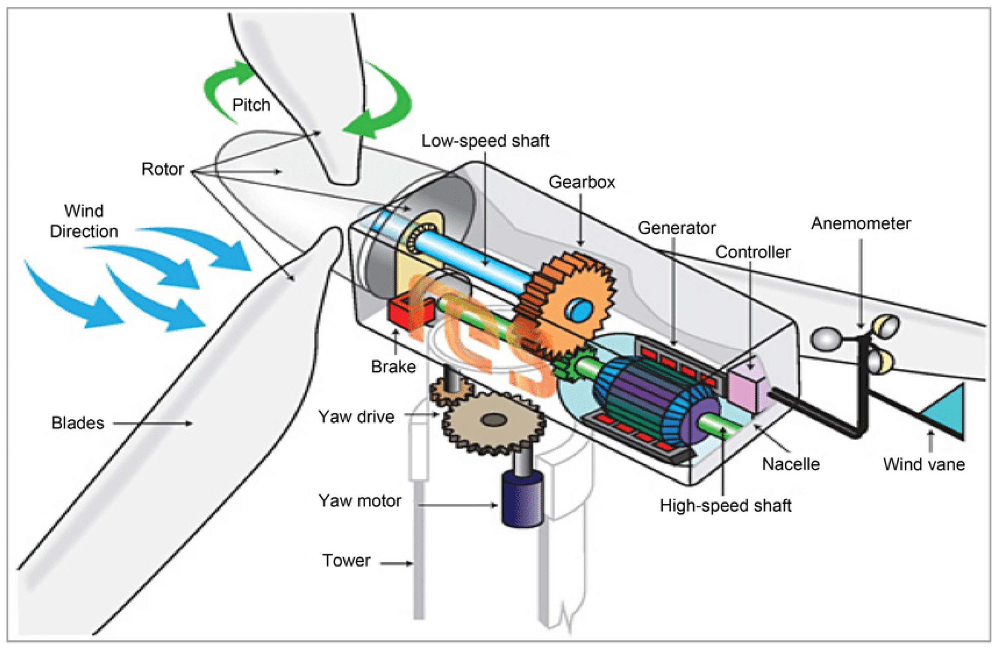
A wind turbine converts the kinetic energy of the wind into mechanical energy and the resulting mechanical energy to electrical energy. As described in Figure 1, the blades, which are aerodynamically optimized to capture the maximum wind power, transfer this power to a rotor hub, connected to the gearbox via the low-speed shaft. This latter allows to transfer the wind energy captured by the turbine to a generator. Then, the generator transforms the rotation energy into electrical energy which is then transferred to a transformer. This latter acts as a link between turbines and distribution grids.

Since wind turbines are expensive equipment, and in order to prioritize research efforts in PdM, it is important to identify what are the critical components. According to a research study by Zhu and Li [30], the gearbox has the greatest failure rate, particularly for offshore wind turbines. It is also found that the generator, the generator bearings and the transformer are also affected by a high failure rate. Considering that these components represent heavy and expensive parts of the wind turbine, any failures affecting them may result in high maintenance cost and production loss.

2.2. Data Description

The considered data set was provided by a global leading company in the energy sector: Energias De Portugal (EDP). The data set, containing Supervisory Control and Data Acquisition (SCADA) [31] measurements, was made available during a wind turbine competition held in 2019 by EDP, and is now open access [32], allowing researchers to develop and compare their PdM strategies on the same framework.

The data set contains measurements from a wind farm composed of five turbines, denoted: $T_{01},T_{06},T_{07},T_{09},T_{11}$. In accordance with the state-of-the-art, the critical components that are considered for monitoring are the gearbox, generator, generator bearings, transformer and hydraulic group.

Each turbine is equipped with sensors, that provide 2-years data ($2016, 2017$), recorded every 10 min, about generator bearing temperatures, oil temperature, pitch angle, generator rpm, etc. For the wind farm, three separated sets of data were given.

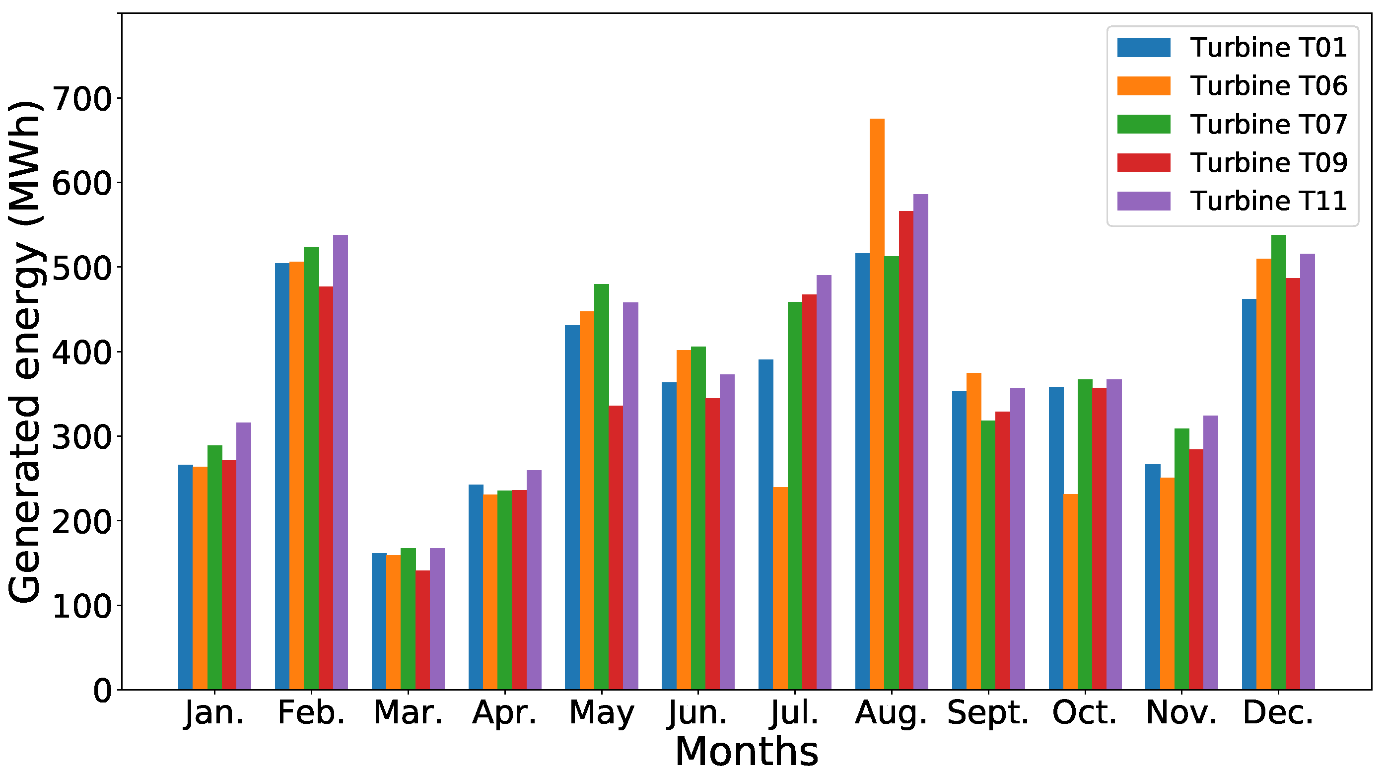
• Sensors data: For each turbine, measurements such as generator speed, blade pitch angle, wind speed and direction, etc., were recorded every 10 min. The average, standard deviation, minimum and maximum of these measurements were stored, for a total of 81 variables. Figure 2 shows one of the useful available parameter in the data set, which is the energy produced by each turbine during 2016.
  It is worth noticing that the quantity of energy produced by the turbine is different and that it varies from month to month. Since the wind turbines have the same characteristics (i.e., same rated power, wind class, cut-in and cut-out wind speed, etc.) and the same components (same characteristics for the rotor, tower, gearbox, and generator), this difference in energy production could be explained by their location in the wind farm or by the occurrence of failures.
• Meteorological mast data: This data set contains measurements of 40 variables related to the environment where the turbines are located, such as wind speed, wind direction, temperature, pressure, humidity, precipitation, and more. For some of the variables, the minimum, maximum, average, and the variance are included. This data was also recorded every 10 min for 2 years (2016 and 2017).
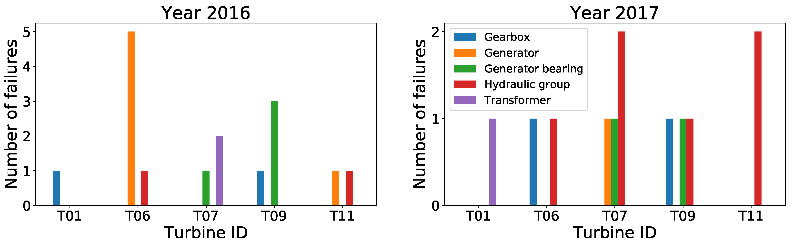
• Failures data: The failures data set provided by EDP covers five components: gearbox, transformer, generator bearing, generator, and hydraulic group. The number and type of failures that affected each turbine during years 2016 and 2017 is summarized on Figure 3 and in

  Table 1. Failure summary.

  Component	T01		T06		T07		T09		T11
  	2016	2017	2016	2017	2016	2017	2016	2017	2016	2017
  - Generator	0	0	5	0	0	1	0	0	1	0
  - Hydraulic Group	0	0	1	1	0	2	0	1	1	2
  - Generator bearing	0	0	0	0	1	1	3	1	0	0
  - Transformer	0	1	0	0	2	0	0	0	0	0
  - Gearbox	1	0	0	1	0	0	1	1	0	0
  Total	1	1	6	2	3	4	4	3	2	2

  .
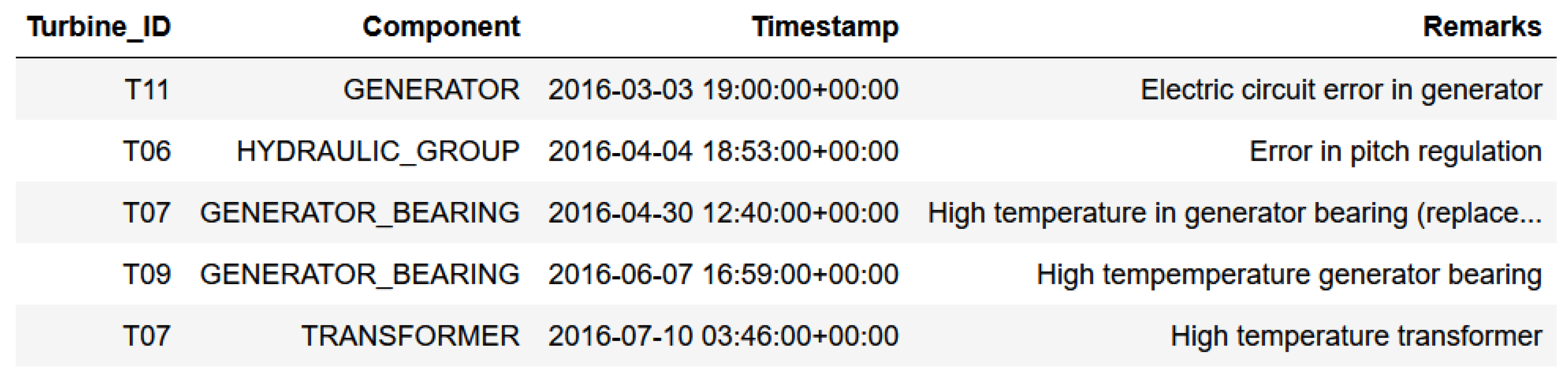
  According to the failure summary (Table 1), one can notice that the component that failed most is the generator (6 times in 2016 and 1 time in 2017), and the turbine with more failures is the $T_{06}$ (6 times in 2016 and 2 times in 2017). Finally, a sample of failure data is shown in Figure 4.
  For each failure, information is given about the turbine in which it occurred, the affected component, the time and day, and a remark explaining the characteristics of the failure.

2.3. Data Preparation

The first step in the data preparation was to combine the measurements from the meteorological mast and sensors data into one data set. For both data sets, the measurements were provided every 10 min. However, for some timestamps, the information was missing in sensors data ($0.9\%$ of records) and in meteorological mast data ($16.9\%$ of records). To successfully concatenate these two data sets, it was necessary to add rows filled with missing values for each missing timestamp. Afterwards, two data sets were merged into one data set containing 121 features.

Thereafter, the two-years long monitored period was divided into the training period (January 2016–July 2017) and the testing period (August 2017–December 2017). This division provided large subset for model training ($79\%$), as well as sufficient testing subset ($21\%$) which contains all types of failures monitored at the considered wind farm.

In order to reduce the risk of overfitting, it is common to keep a part of the testing set aside for the final assessment of ML algorithm [33]. The remaining part is used for evaluation of the various choices made during the design of an ML system. Since an ML model we used is not time-dependant, we sampled the half of the data from the testing period randomly and used it as a validation set. The remaining half was used as a test set for evaluation of the precision of the final model. The chosen type of split ensures, that both healthy and faulty data points are present in the validation and test sets for each considered component.

In the experiments, we adopted predictive maintenance task defined during the competition [32]—to predict the failures of components two months before their occurrence. The target variables for each component were designed using information from failures data. For each considered component of wind turbines, we defined two types of target variables: binary target value (classification task) and continuous target value (regression task). In order to compare the results obtained using different types of targets on the same scale, we transformed continuous predictions to the binary values before the evaluation of results, and thus we were able to use classification evaluation metrics for both tasks.

3. Materials and Methods

ML allows computers getting insights from data without being explicitly programmed. An effective ML system is able to provide reliable predictions for the task it was designed for on the data it did not encounter during training phase. The design of such system usually requires iterative searching for the best ML model by fitting various models to processed raw data.

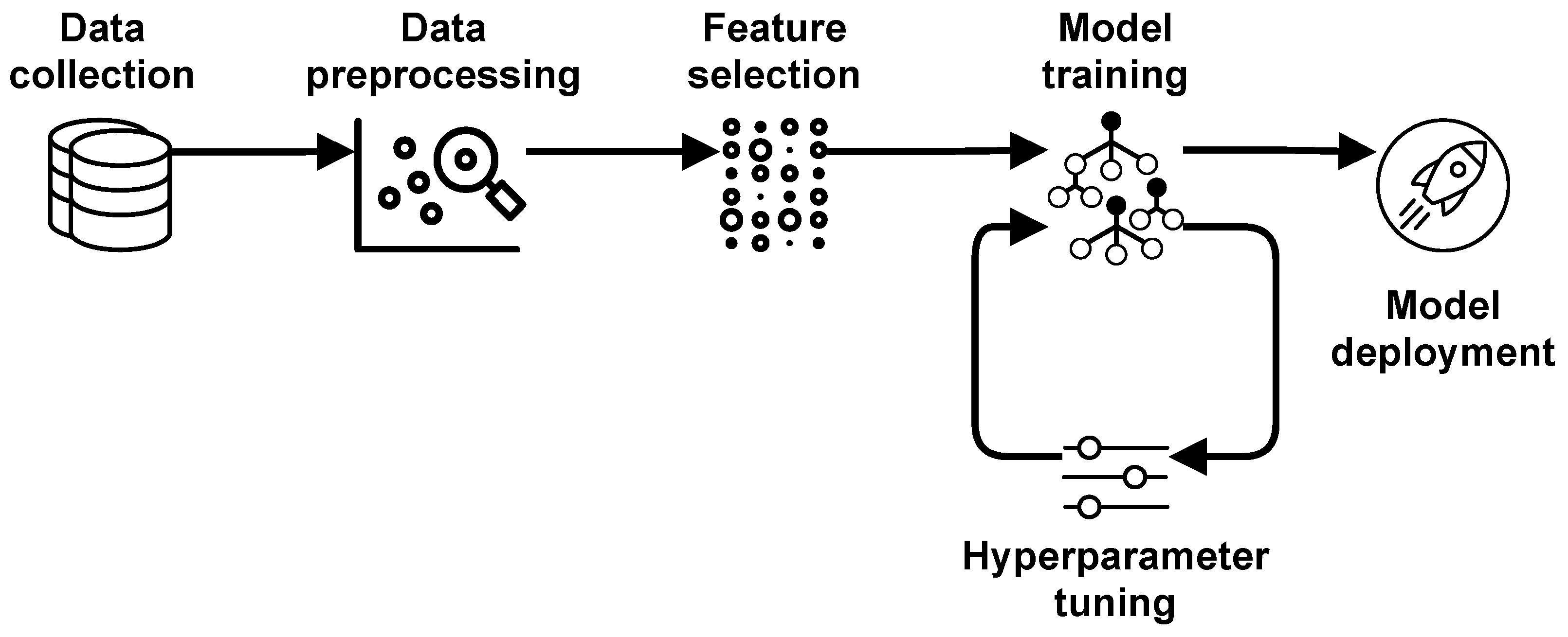
The approach to the design of ML models, which is currently prevalent in ML community, is model-centric, i.e., centered around searching for the best model with a fixed set of considered features. Figure 5 provides an example of pipeline for model-centric ML. The main characteristic of this approach is that all steps preceding model training are one-time procedures. They are executed only once at the beginning of ML model design. The core part of this methodology is model training with hyperparameter tuning.

The main drawback of the model-centric methodology is not taking into account that the precision of the resulting model depends not only on the chosen type of model and its hyperparameter setting, but also on the quality of the data entering the model. Oftentimes, data contains features that do not improve the precision, but, even more alarming, contribute to overfitting. Furthermore, some features may contain erroneous data, which may be problematic to discover for larger data sets. In both situations, the precision of the resulting model is diminished, and it cannot be improved merely by hyperparameter tuning, however extensive it would be.

The most common approach to deal with this issue is to collect more data to compensate for potential weaknesses. However, for many areas, collecting huge amounts of data is not feasible. Therefore, it is important to design and explore methods to improve data we already have at our disposal. Techniques which aim to improve the performance of ML models by improving the data which enters into these models are referred to as data-centric ML. Needless to say, that concentrating solely on data without searching for the best model will most likely not improve the precision of the final system. However, enriching the traditional model-centric approach by mindful choosing of features to consider and improving their quality tend to not only increase the precision of the final ML model, but also to reduce the computational time of training procedures.

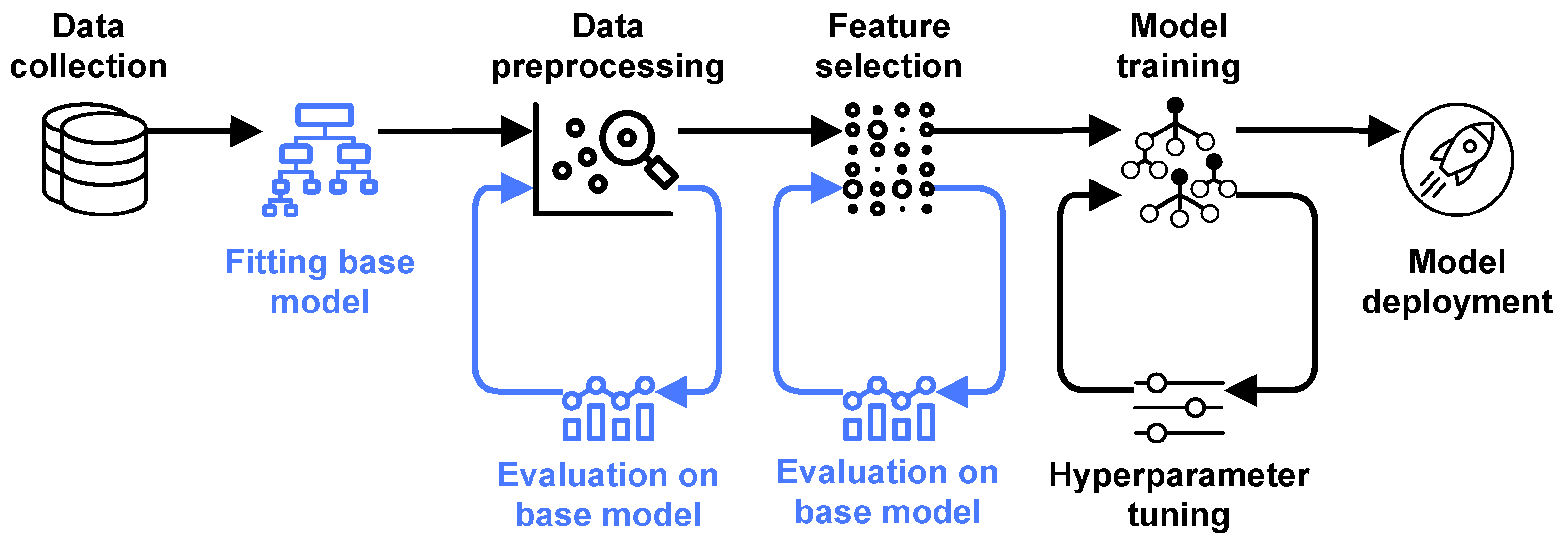
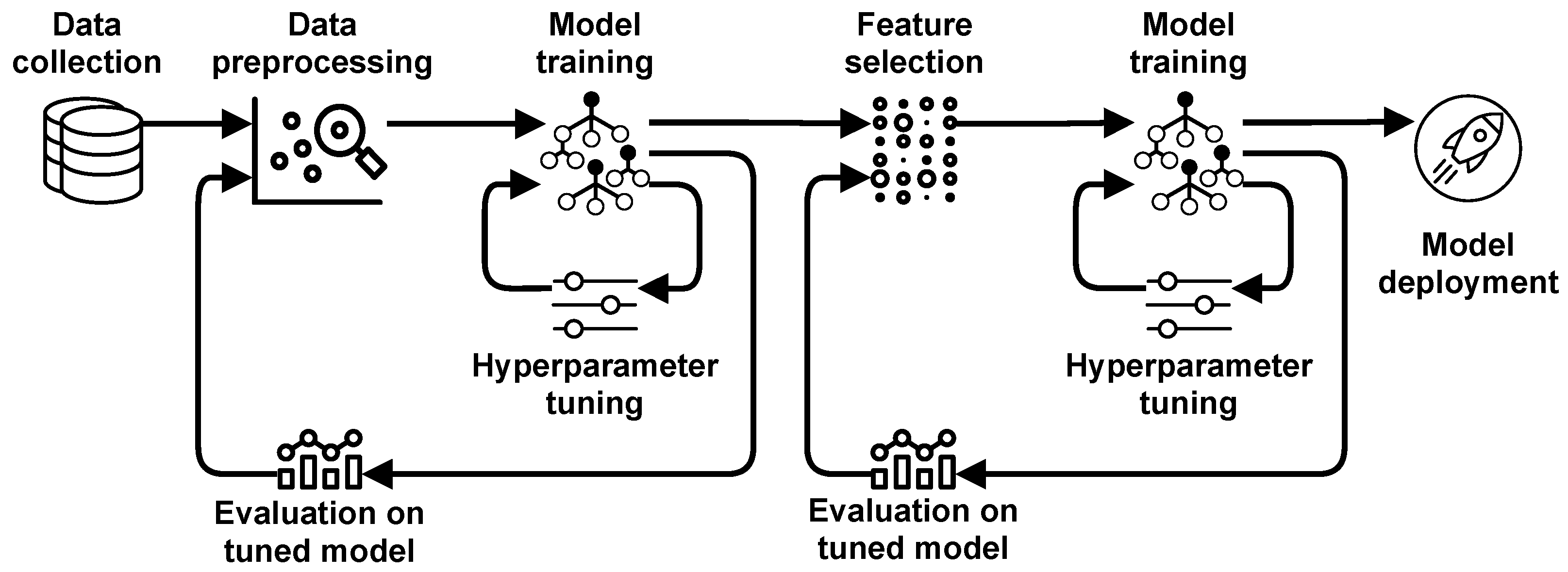
3.1. The Proposed Data-Centric ML Methodology

The methodology we propose in this paper is shown on Figure 6. Unlike the pipeline shown on Figure 5, here data preprocessing and feature selection are not one-time steps, but they are executed repetitively. Each strategy is implemented and evaluated on the base model. Consequently, the best strategy is defined and used. Then, several strategies for feature selection are implemented and evaluated on the base model. The best feature selection strategy is chosen for the model training phase.

It is important to choose an appropriate evaluation metric to use throughout the pipeline. The variables which enter the evaluation step are binary. The most widely used metric for this type of predictions is accuracy, which is calculated as a ratio between the number of correct predictions and the total number of predictions. However, this metric provides overoptimistic estimate of performance for skewed data sets, i.e., the data sets with imbalanced number of representatives of each class. Predictive maintenance in general tends to operate with skewed data sets, since we have much more healthy data than faulty data. Therefore, accuracy may not be the best choice for the evaluation of precision in the pipeline.

In binary classification, we deal with four possible prediction outcomes:

• True positives (TP)—we predict the positive outcome, and it is indeed positive;
• True negatives (TN)—we predict the negative outcome, and it is indeed negative;
• False positive (FP)—we predict the positive outcome, but the outcome is negative;
• False negative (FN)—we predict the negative outcome, but the outcome is positive.

Using the outcomes specified above, we can define accuracy as:

$$\mathrm{Accuracy}=\frac{\mathrm{TP}+\mathrm{TN}}{\mathrm{TP}+\mathrm{TN}+\mathrm{FP}+\mathrm{FN}}·100\%$$

(1)

Alternative metrics, which are commonly used with skewed data, are precision and recall. Precision is a fraction of true positive examples among all examples that the model classified as positives:

$$\mathrm{Precision}=\frac{\mathrm{TP}}{\mathrm{TP}+\mathrm{FP}}·100\%$$

(2)

Recall, which is also called sensitivity, is a fraction of true positive examples among all positive examples:

$$\mathrm{Recall}=\frac{\mathrm{TP}}{\mathrm{TP}+\mathrm{FN}}·100\%$$

(3)

Depending on what is more important in a given application, one can choose precision or recall as an evaluation metric for skewed data. If improving both metrics simultaneously is required, one can use their harmonic mean, which is often referred to as F1 score:

$$\mathrm{F}1=2·\frac{\mathrm{Precision}·\mathrm{Recall}}{\mathrm{Precision}+\mathrm{Recall}}=\frac{\mathrm{TP}}{\mathrm{TP}+\frac{1}{2}(\mathrm{FP}+\mathrm{FN})}·100\%$$

(4)

We used the F1 score as an evaluation metric throughout the pipeline. Its value is evaluated on the validation set to reduce the chance of overfitting.

3.1.1. Fitting Base Model

The initial step of the proposed methodology is to find the base model which will be used throughout the pipeline. The choice of its type is predetermined by the type of model we intend to use in model training phase. Since we chose to use the DT for PdM, it is appropriate to use the same model as the base model. However, the scale of models we can choose in model training phase using the proposed approach is not limited to only DT, we can use any algorithm derived from it, i.e., RF, XGBoost, etc.

3.1.2. Data Preprocessing

In this step, various preprocessing strategies are implemented and evaluated on the base model. Data preprocessing often incorporates important choices which are usually done rather intuitively. These choices include:

• Strategy for dealing with missing values;
• Design of an efficient target variable;
• Design of new features;
• Data cleaning procedures.

In the proposed data-centric methodology, each considered strategy is evaluated on a base model. Consequently, the best combination of strategies is chosen as a preprocessing routine for row data. Preprocessed data are then used in the next step of the pipeline.

3.1.3. Feature Selection

Oftentimes, real-world data contains wide set of features, and not all of them are informative for the process they are meant to describe. Presence of non-informative features not only prolongs the computation time, but it also contributes to overfitting of the final models. Therefore, selection of the optimal set of features from the data set can have an enormous influence on the performance of ML models.

The commonly used method for feature selection is manual selection based on the domain knowledge. However, using this approach, some features with high predictive value can be excluded from the analysis just because this value has not yet been established. Moreover, for some applications of ML, obtaining deep domain knowledge can be problematic.

Using the proposed data-centric methodology, we can implement various feature selection techniques on the preprocessed data set and evaluate their performance. The setting which provides the best precision on the validation set is then chosen for the model training step.

3.1.4. Model Training

Model training step is executed in the same manner as in the model-centric approach to ML. A chosen ML model is fitted to the data set with various settings of hyperparameters. The setting that provides the best performance on the validation set is chosen as the final model. The precision of the final model is reported on the test set, which was not used in the pipeline.

3.2. Data Preprocessing Steps Applied on the Case Study Data

During data preprocessing step with application on the case study data, we focused on two tasks: dealing with missing values and the design of an efficient target variable.

For missing values treatment, we chose three strategies for the experimental part:

• Simple imputation of missing values using backward and forward filling;
• Extended imputation of missing values (adding two binary features which reflect whether a row was missing in the Signals data set and data set from the meteorological mast);
• Removing rows which were missing in both Signals data set and data set from meteorological mast.

For each component, the best strategy was chosen according to the results of evaluation on the base model.

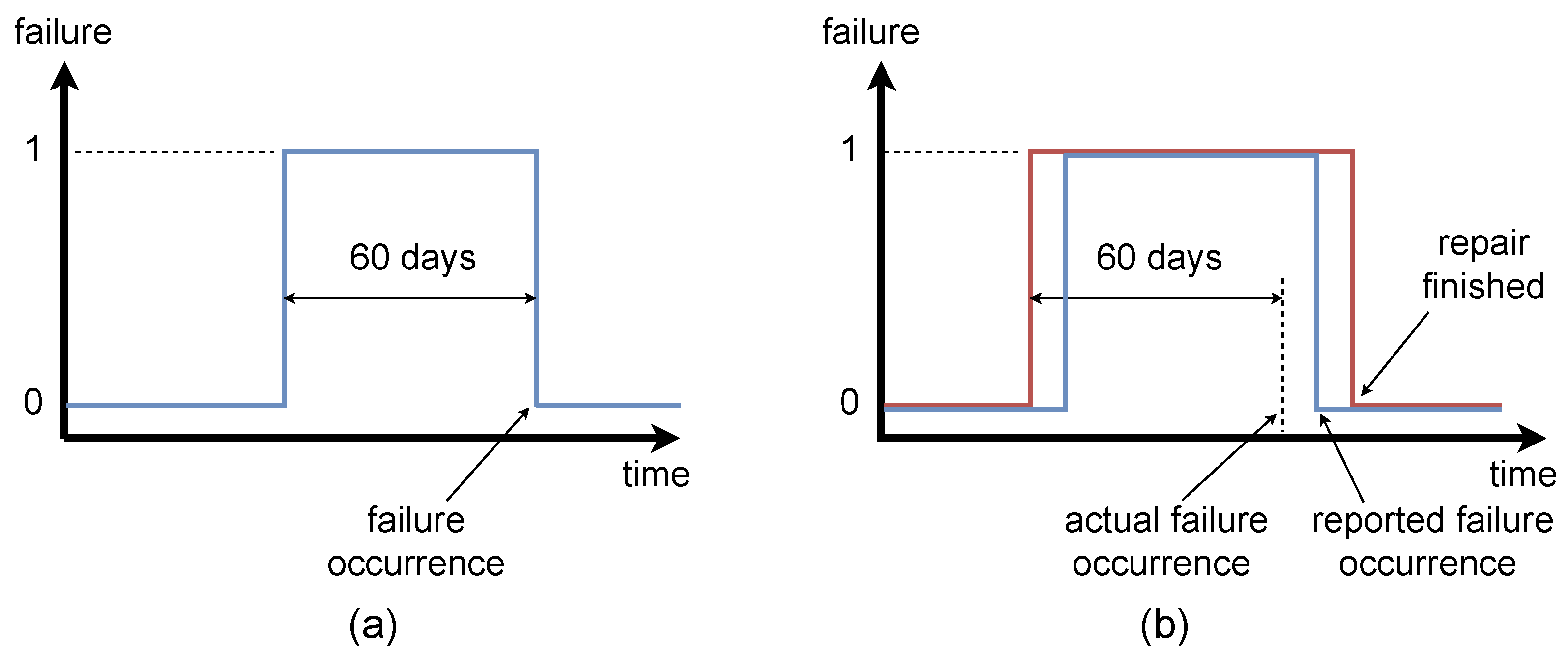
Regarding the design of target variables, we chose two types: binary variable (which implied solving a classification task) and continuous variable (which implied solving a regression task). The first set of target variables was designed for each component from the information stored in the failures data set in the following manner:

• Binary variable—the target value is equal to “1” for 60 days before the failure occurred, and it is equal to “0” for healthy condition of a component, see Figure 7a.
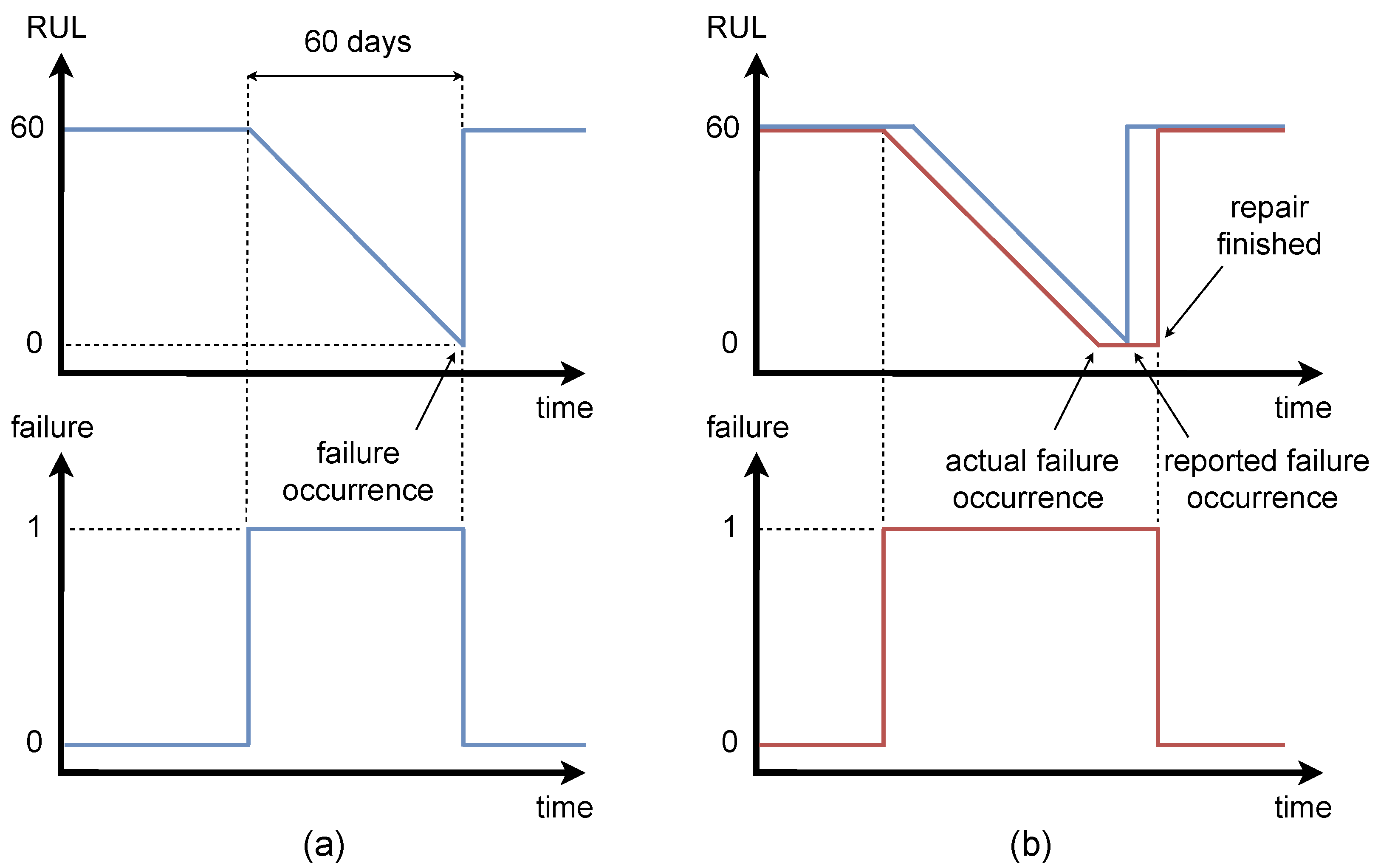
• Continuous variable—the target is represented by the value of Remaining Useful Life (RUL) of a component, see Figure 8a. The value of the RUL is equal to zero when the failure occurs. Its descent lasts 60 days before the failure. The value of target for healthy condition is equal to 60 days (1440 h).

In order to compare the predictions from the classification and regression algorithms on the same scale, we transformed the continuous target to binary values before the evaluation of results in the manner presented on the bottom plot of Figure 8a. Consequently, we were able to apply metrics for classification task on the results from a regression algorithm.

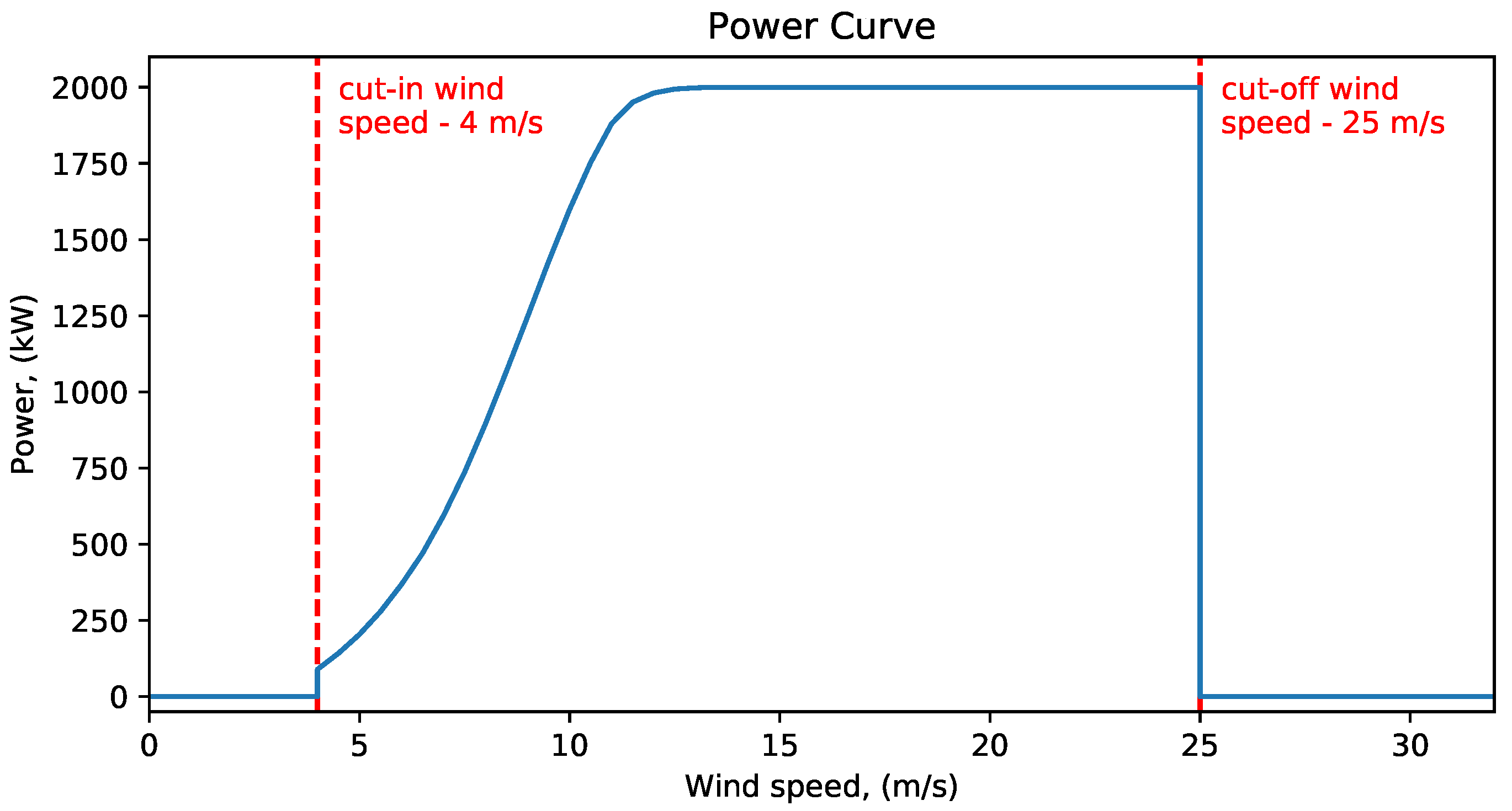
One of the key approaches implemented in data-centric ML is improvement of target variables. Therefore, we constructed the second set of target variables by the manual improvement of the initial targets. For this purpose, we analyzed the signal flow of the power produced on turbines in the vicinity of a fault. To properly analyze the signal, it is important to additionally take into consideration the wind speed in the same time segment, since the turbine can be inactive not due to the fault, but simply due to the absence of the wind. The power curve of the considered wind turbines is shown on Figure 9. From the figure, we can see that a turbine will not produce power for wind speed below 4 m/s or above 25 m/s.

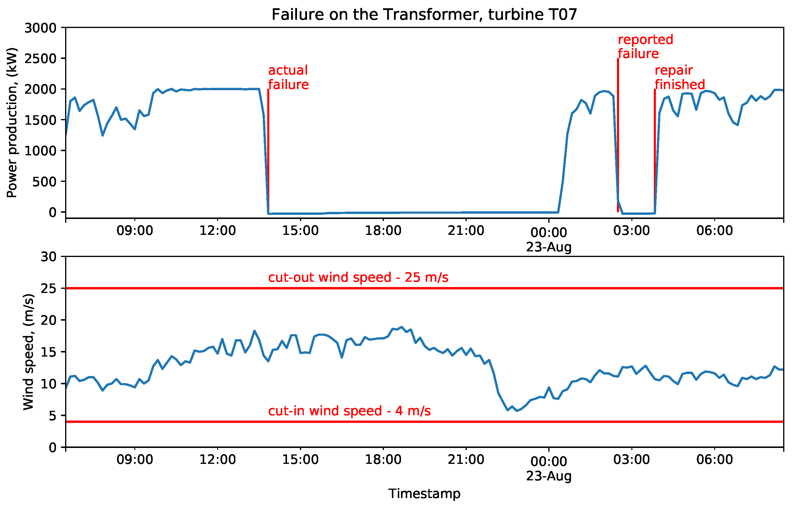
The example of late report of the failure is shown on Figure 10. It is evident, that the failure occurred more than twelve hours before the reported failure time, since the turbine did not produce power while the wind speed was in its active range. The improvement of binary targets with this information is shown on Figure 7b and of continuous targets on Figure 8b.

We applied this strategy on every failure in the failure data set. Unfortunately, the actual occurrence of failure was not as evident as on Figure 10 for every considered case. In particular, in the absence of wind, it is hard to guess the actual time of failure occurrence. To assure that the improved set of features has a potential to improve the performance of the final model, we implemented both sets of target values and evaluated them on the base model in accordance to the proposed data-centric methodology. Consequently, we chose the best set of features for each component and each considered task (classification and regression).

3.3. Feature Selection Techniques Used on the Case Study Data

Before implementation of feature selection techniques, it was necessary to exclude features which evidently do not have any predictive value. We excluded the following features:

• Features with zero variance (constants);
• Features with low variance (${\sigma }^2<0.0001$);
• Technical parameters of sensors (sampling rates, offsets, etc.).

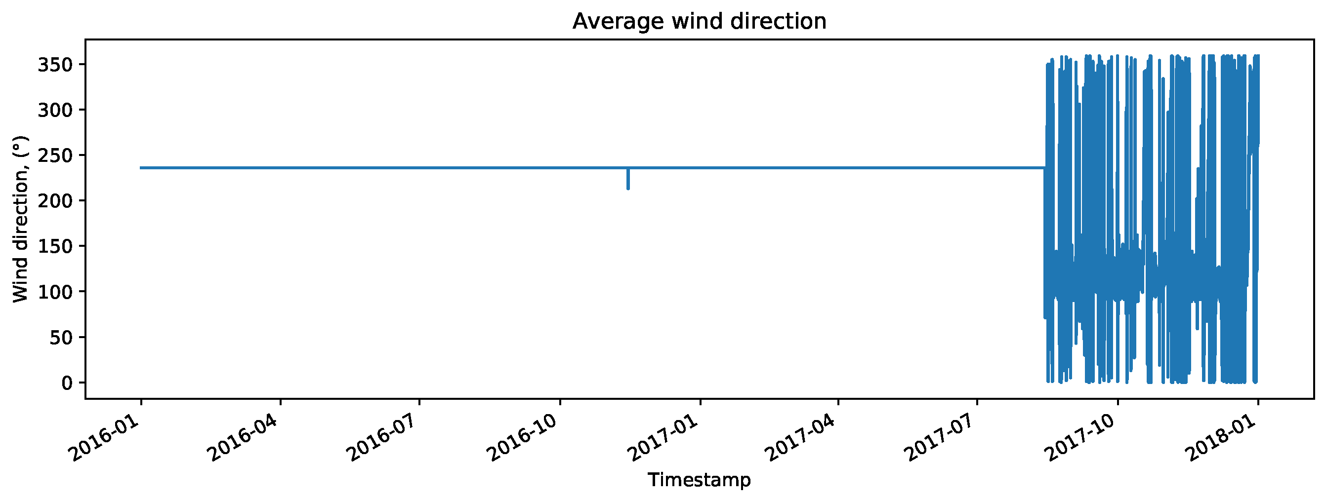
During data exploration, it was discovered that the sensor which measures wind direction on the meteorological mast was broken for almost entire training period. One of the features associated with this sensor is shown on Figure 11. Therefore, we excluded all features associated with this sensor from the data set. The resulting set of features for further consideration consisted of 99 features.

Furthermore, it was discovered that the data set contains numerous redundant features. For many variables, the information about their minimal, maximal and average values during 10-min-long measurement window was stored. These features are clearly highly correlated, and they increase computational time and can contribute to overfitting. Therefore, we consider feature selection a crucial step for the case study data.

The first feature selection technique we implemented was manual selection of features. Using this approach, we kept only information about the average values of every considered variable in the data set. The quality of the resulting set of features was evaluated on the base model.

Then, we implemented five commonly used techniques to decrease the number of features entering an ML model: feature importance selector, high correlation filter, mutual information selector, Principal Component Analysis (PCA) and Independent Component Analysis (ICA). Each of these techniques has its own tuning parameter: threshold for a filter, the number of considered features for a selector, and the number of considered components for PCA and ICA. The choice of these parameters is usually intuitive, which brings a substantial subjective factor into the design of an ML system. Applying the proposed data-centric approach, we can evaluate different values of the tuning parameter on the base model and pick the one which results in the best performance. The range of considered tuning parameters for each technique is listed in

Table 2. Tuning parameters considered in feature selection techniques.

Technique	Tuned Parameter	Considered Range
Feature importance selector	number of features	$[10,20,\dots ,90]$
High correlation filter	threshold	$[0.5,0.6,\dots ,0.9]$
Mutual information selector	number of features	$[10,20,\dots ,90]$
Principal component analysis	number of components	$[10,20,\dots ,90]$
Independent component analysis	number of components	$[10,20,\dots ,50]$

.

• Feature importance selector. Feature importance is a class of techniques that is used for estimation of the relative importance of each feature in a data set during prediction of the target variable. The relative importance is expressed by a score which is computed according to a chosen technique. In the DT, the importance of a feature is expressed by the normalized total reduction a feature brings to a criterion (a function that measures the quality of a split). After calculating the relative importance of each feature, we obtain the ranking of features in relevance to a given target. Thereafter, we select a certain number of the most informative features for prediction of a target variable.
• High correlation filter. High correlation filter chooses the subset of features which are at worst weakly correlated and at best uncorrelated. In order to implement high correlation filter, we search for pairs of highly correlated features. For each pair, we choose a feature which has higher correlation with a target. The choice of the threshold to use to state that features are highly correlated, is a tuning parameter for this technique.
• Mutual information selector. Mutual information between a feature and a target expresses the reduction in uncertainty that the knowing of a feature brings to a target. Similarly to high correlation filter, mutual information measures the dependence between two features. However, the latter covers both linear and non-linear dependencies. After calculating the mutual information of each feature, we obtain the ranking of features in relevance to a given target. Thereafter, we select a certain number of the most informative features for prediction of a target variable.
• Principal component analysis. PCA belongs to a class of dimensionality reduction techniques. Theses techniques, in contrast to filters and selectors, do not exclude features, but rather create a new set of variables (called components) from all features. In PCA, we calculate principal components, which are represented by linear combinations of the original features. The technique aims to reduce feature space with minimal loss of information by retaining the variance contained in features. Before implementing PCA, a decision regarding the number of principal components to extract from data has to be made.
• Independent component analysis. ICA is another representative of dimensionality reduction techniques. In ICA, we calculate independent components, which are represented by linear combinations of some unknown latent variables which are assumed to be independent. In contrast to PCA, which searches for uncorrelated factors, ICA searches for independent factors. Before implementing ICA, a decision regarding the number of independent components to extract from data has to be made.

After choosing the best setting for feature selection techniques for both continuous and regression tasks, we pick the best combination for each considered component. This combination is then used during model training.

3.4. Implementation of the Proposed Methodology

We implemented the proposed data-centric methodology using functions from scikit-learn module [34]. We chose to use DT [35] as a base model for verification of the methodology since it is one of the most commonly used ML algorithms for condition monitoring in wind turbines [9] with relatively low computational demands.

Implementation of various feature selection techniques using functions from scikit-learn is straightforward. The time required for computation is relatively low for all techniques except mutual information, which is more time-demanding. In addition, for the regression task, calculation of mutual information is known to be generally challenging [36] with high demands on the internal memory. To overcome the latter issue, we calculated the mutual information on the subset of data. To generate the subset, 10% of entries were randomly picked from the training set.

The most computationally expensive step in the pipeline is model training, which consists of searching for the optimal set of hyperparameters for an ML model.

4. Results

In this section, the results are presented and evaluated in accordance to the pipeline from Figure 6.

4.1. Fitting Base Model

As an initial step in data analysis, base models for each component were computed. For this purpose, the DT was fitted to the original data set with imputed missing values using backward filling for both classification and regression tasks. The obtained models were used for evaluation of the data preprocessing and feature selection strategies.

4.2. Data Preprocessing

In the data preprocessing step, several preprocessing strategies were tested for each component. The values of F1 score for each strategy-component combination are presented in

Table 3. Values of F1 score on validation set for considered data preprocessing strategies. Values are presented in percents.

Strategy	Generator	Hydraulic Group	Generator Bearing	Transformer	Gearbox
Classification task
1. Initial target + backward filling	0.20	20.62	8.80	0.68	7.95
2. Initial target + forward filling	0.23	18.14	6.43	0.27	8.16
3. Improved target + backward filling	0.04	19.84	11.17	2.20	7.69
4. Improved target + forward filling	0.18	17.81	7.96	0.00	8.91
5. Remove rows filled with NaNs	0.21	20.46	11.17	2.20	8.91
6. Extended imputation	0.18	20.03	11.85	2.17	7.34
Regression task
1. Initial target + backward filling	5.76	40.08	7.87	6.26	37.62
2. Initial target + forward filling	5.94	40.00	7.13	6.62	33.18
3. Improved target + backward filling	6.60	41.84	10.07	6.25	33.95
4. Improved target + forward filling	7.07	38.94	8.63	6.70	33.61
5. Remove rows filled with NaNs	7.07	41.53	10.07	6.74	37.61
6. Extended imputation	6.80	42.05	9.92	6.62	23.81

. First, the target feature to consider (initial or improved, as shown on Figure 7 and Figure 8) in combination with imputation strategy (backward or forward filling) was chosen for each component. The chosen combinations provided the highest values of F1 score on the validation set (highlighted with bold text in Table 3). Consequently, we experimented with removing rows which were missing in the original data set and the strategy of extended imputation (adding binary variables which reflect whether the row was missing in the data from the turbines or from the meteorological mast). Settings which provided improvement in precision are highlighted with bold text in Table 3.

For all components except Generator Bearing, using of continuous target variables yielded much more precise results. In some cases, for example for Transformer with binary targets, the choice of imputation method had big impact on the precision. For the majority of component-task combinations, extended imputation and removing rows initially filled with missing values did not help, whereas manual improvement of targets justified itself.

As a result of the experiments, the optimal data preprocessing algorithm was established for each component:

• Generator
  • Classification task: use initial target variable and imputation using forward filling.
  • Regression task: use improved target variable and imputation using forward filling, remove rows initially composed of missing values.
• Hydraulic Group
  • Classification task: use initial target variable and imputation using backward filling.
  • Regression task: use improved target variable and extended imputation using backward filling.
• Generator Bearing
  • Classification task: use improved target variable and extended imputation using backward filling.
  • Regression task: use improved target variable and imputation using backward filling, remove rows initially composed of missing values.
• Transformer
  • Classification task: use improved target variable and imputation using backward filling.
  • Regression task: use improved target variable and imputation using forward filling, remove rows initially composed of missing values.
• Gearbox
  • Classification task: use improved target variable and imputation using forward filling.
  • Regression task: use initial target variable and imputation using backward filling.

4.3. Feature Selection

After implementation of the appropriate preprocessing algorithm on every component-task combination, we shifted to the feature selection step. After discarding non-informative features (refer to Section 3.1.2 for more details), the remaining set of features consisted of 101 features for the data sets which underwent extended imputation and 99 features for the remaining data sets. Various feature selection techniques were applied on these subsets for potential reduction of the amount of considered features.

The first considered feature selection technique was manual feature selection. Since many features in the data set convey similar information (i.e., minimum, average and maximum values for a given variable), we manually picked only features corresponding to the average values of variables. Implementation of this intuitive approach however did not have the expected improvement in precision. On the contrary, the precision decreased for all component-task combinations except the Generator with continuous target variable (refer to

Table 4. Values of F1 score on validation set for the best settings of considered feature selection techniques. Values are presented in percents.

Technique	Generator	Hydraulic Group	Generator Bearing	Transformer	Gearbox
Classification task
Base model (after data preprocessing)	0.23	20.62	11.85	2.20	8.91
Manual feature selection	0.04	16.68	5.36	1.24	6.71
Feature importance	0.20 (10 feat.)	21.19 (10 feat.)	11.85 (50 feat.)	2.91 (20 feat.)	9.35 (80 feat.)
High correlation filter	3.55 (thr. = 0.5)	15.20 (thr. = 0.9)	20.00 (thr. = 0.6)	2.76 (thr. = 0.5)	15.14 (thr. = 0.7)
Mutual information	1.92 (10 feat.)	20.59 (70 feat.)	16.07 (70 feat.)	2.43 (70 feat.)	17.58 (30 feat.)
PCA	5.63 (20 comp.)	6.87 (80 comp.)	24.16 (10 comp.)	2.90 (30 comp.)	10.59 (30 comp.)
ICA	4.89 (20 comp.)	13.97 (50 comp.)	23.65 (50 comp.)	3.44 (30 comp.)	12.28 (30 comp.)
Regression task
Base model (after data preprocessing)	7.07	42.05	10.07	6.74	37.62
Manual feature selection	7.17	40.98	5.44	4.78	30.46
Feature importance	7.26 (20 feat.)	42.11 (90 feat.)	11.54 (60 feat.)	7.01 (50 feat.)	37.82 (80 feat.)
High correlation filter	5.00 (thr. = 0.7)	37.89 (thr. = 0.8)	10.46 (thr. = 0.9)	7.36 (thr. = 0.8)	37.07 (thr. = 0.9)
Mutual information	7.61 (40 feat.)	44.38 (40 feat.)	12.49 (20 feat.)	7.21 (60 feat.)	35.10 (20 feat.)
PCA	6.92 (70 comp.)	35.71 (60 comp.)	6.30 (40 comp.)	3.09 (30 comp.)	28.06 (30 comp.)
ICA	6.87 (30 comp.)	36.32 (50 comp.)	5.74 (50 comp.)	3.09 (30 comp.)	27.35 (10 comp.)

where the precision achieved with manual feature selection, as well as the precision of base models obtained in the data preprocessing step, are presented). It confirms the necessity of applying feature selection techniques to the data set.

Five feature selection techniques with various values of the tuning parameters were implemented for each component-task combination. The considered values for the tuning parameters (i.e., number of features, number of components and filter threshold) for each feature selection technique are shown in Table 2. The F1 scores of the best settings (i.e., the ones that provided the maximum value on the validation set) for each feature selection technique are given in Table 4. As it can be observed, not all feature selection techniques were effective for every component-task combination, but at least one among them provided the improvement in precision in every considered setting. Noteworthy, none of the considered techniques provided generally bad results. For each component, the technique with the maximum value of F1 score was chosen as the optimal one (highlighted with bold text in Table 4). The subset of features obtained from the corresponding technique was used for training of the final ML model for each considered component.

4.4. Model Training and Evaluation

In the model training step, five DTs were trained with hyperparameter tuning. The best set of hyperparameters was chosen on the validation set using F1 score as an evaluation metric. The metrics of the final model were evaluated on the test set, which was not used earlier in the pipeline. Evaluation metrics on both validation and test sets for each model are presented in

Table 5. Model training summary. Values are presented in percents.

Model	Validation Sets				Test Sets
	Accuracy	Precision	Recall	F1 Score	Accuracy	Precision	Recall	F1 Score
	Generator
Base model	14.38	2.97	99.04	5.76	14.61	3.09	98.94	5.99
Optimal set of features	26.61	3.98	85.08	7.61	26.95	4.17	84.26	7.94
Decision tree after hyperparameter tuning	43.92	4.88	79.92	9.20	44.21	5.11	79.16	9.59
	Hydraulic Group
Base model	52.16	27.60	73.05	40.08	52.28	27.76	73.24	40.26
Optimal set of features	59.48	31.76	73.67	44.38	59.60	31.90	73.68	44.53
Decision tree after hyperparameter tuning	57.69	31.37	78.14	44.77	57.82	31.49	77.95	44.85
	Generator Bearing
Base model	85.86	13.40	6.55	8.80	85.94	12.73	6.12	8.27
Optimal set of features	95.74	32.66	19.17	24.16	95.59	34.86	20.74	26.00
Decision tree after hyperparameter tuning	96.87	67.64	22.50	33.77	96.77	68.98	24.62	36.29
	Transformer
Base model	79.46	3.34	49.54	6.26	79.31	3.11	46.57	5.83
Optimal set of features	76.23	3.89	68.06	7.36	76.23	4.06	71.34	7.69
Decision tree after hyperparameter tuning	87.32	4.68	42.02	8.42	87.11	4.48	40.84	8.08
	Gearbox
Base model	53.65	23.88	88.57	37.62	53.59	23.68	88.86	37.39
Optimal set of features	55.29	24.22	86.18	37.82	55.21	24.06	86.79	37.67
Decision tree after hyperparameter tuning	55.35	24.25	86.17	37.85	55.27	24.10	86.89	37.73

.

Evaluation metrics of the final models on the validation sets show certain degree of improvement compared to the base model. For Gearbox component, the improvement of the F1 score over the base model is slight (less than 1%). For Generator, Hydraulic Group and Transformer, the improvement is more noticeable (several percents). For Generator Bearing, the F1 score of the final model is almost four times higher than that of the base model. The values of F1 scores for the test sets were higher or at worst comparable with those obtained on the validation sets, which suggests good generalization abilities of the final models.

5. Discussion

The results suggest that the proposed data-centric methodology is effective for the evaluation of various data preprocessing strategies and feature selection techniques in an ML pipeline. It provides a framework for choosing the most appropriate sequence of preprocessing steps, as well as the optimal set of features to use in the ML model.

As it can be seen from Table 3, various data preprocessing choices can have a tangible effect on the performance of ML models. Moreover, the manual improvement of target variables applying domain knowledge was shown to be a promising data-centric strategy. As it can be seen from Table 4, manual feature selection can have a counter-productive effect on the performance of ML models. The implementation of feature selection techniques is a perspective alternative to this approach. In addition, parameter tuning of these techniques can significantly improve their performance. Evaluation metrics of the final models on the test sets (from Table 5) were compared to the results obtained by Eriksson [24], who developed ML models for the same case study using the model-centric approach. The comparison is shown in

Table 6. Comparison of the results from model-centric and data-centric approach. Values are presented in percents.

Component	Model-Centric Approach [24]				Data-Centric Approach
	Accuracy	Precision	Recall	F1 Score	Accuracy	Precision	Recall	F1 Score
Generator	80.79	0	0	0	44.21	5.11	79.16	9.59
Hydraulic group	70.65	53.29	19.08	28.10	57.82	31.49	77.95	44.85
Generator bearing	81.11	18.72	40.96	25.70	96.77	68.98	24.62	36.29
Transformer	88.21	4.26	5.70	4.88	87.11	4.48	40.84	8.08
Gearbox	82.64	29.18	48.09	36.32	55.27	24.10	86.89	37.73

. In the original publication, the values of F1 score were not included into evaluation metrics of the final models ([24], Table 4.2). Therefore, we computed their values using Formula (4). The author implemented various ML algorithms (linear regression, DT, RF, gradient boosted tree, multilayer perceptron, SVM) with improvement techniques (stacking and boosting) on the case study data. The results presented in Table 6 correspond to the best models obtained using model-centric approach, namely stacked multilayer perceptron algorithm. The data-centric methodology implemented in this article provided noticeably better results with a simpler model (a DT). To improve clarity, the better value for each considered pair of metrics is highlighted with bold text in Table 6. The values of F1 score were higher for all considered components while the values of precision and recall were mostly better. Accuracy was mostly lower for the data-centric approach, but as it was discussed in Section 3.1, this metric is misleading for skewed data sets.

The obtained results can be further improved by using more sophisticated models. Indeed, training of RF, XGBoost or other ML algorithms based on DTs can be applied on the discovered optimal subset of features.

Data-centric paradigm is a novel trend that is gaining in popularity in ML community [25]. As implementation of ML models is becoming more and more straightforward using modern tools, researchers can invest more effort into improving the data to enhance the quality of the final ML models. In addition, the improvement of data quality leads to the decrease in demands on its quantity, which can be beneficial for those fields in which collecting huge data sets is non-feasible.

The current view of the data-centric paradigm in ML community is to implement the whole ML cycle for each considered data-oriented setting [26], i.e., data preprocessing and feature selection steps. Adaptation of this approach for the ML pipeline from Figure 5 is shown on Figure 12. Implementation of this approach increases the required computation time enormously since parameter tuning step is required in each iteration.

The originality of the data-centric methodology proposed in this paper is in the evaluation of each considered setting on a base model, as shown on Figure 6. As hyperparameter tuning is not required in each iteration, the required computation time is decreased considerably compared to the fully-cycled data-centric approach presented on Figure 12.

The proposed data-centric methodology provides a generic approach to optimization of the data-oriented steps in ML pipeline. It can be used with a wide range of data preprocessing strategies and feature selection techniques, in addition to the ones presented in this article. One of the main advantages of the methodology is that it is not domain-specific and thus it can be applied in various fields. Moreover, its implementation does not require expert knowledge in a considered domain due to its semi-automatic nature.

The disadvantage of the proposed methodology compared to the pure model-centric approach is the prolongation of data preparation steps in an ML pipeline. However, compared to required computation time for model training step, this increase is not substantial. Further disadvantage is adding a possible overfitting cause to an ML pipeline which can occur due to computation of the evaluation metric on the same validation set in each considered setting. This overfitting can be be easily detected during final evaluation on the test set and can be eliminated by enhancing the evaluation step through cross-validation techniques.

6. Conclusions

This paper has proved the benefit of a data-centric ML methodology for making wind turbines more reliable, by predicting the RUL more accurately and thus, contributing to the global efforts of tackling climate change. In practice, the RUL information is used to make decisions about the maintenance scheduling of wind turbines, through several actions associated to different costs: inspection, replacement or repair. Based on the methodology’s predictions and associated maintenance costs, a total PdM saving can be calculated to evaluate the PdM strategy.

Among the perspective directions for further research, we can highlight the implementation of more sophisticated ML models enriched with the proposed data-centric methodology. In particular, for the task of PdM of wind turbines, it can be beneficial to implement the methodology with ML algorithms, which perceive data sets as time series, such as long-short-term memory.

The proposed methodology can be used to enhance the precision of ML models beyond the application considered in this article. In addition to its generalizability over various domains, it can also be used in conjunction with wide range of data-oriented strategies.