
Optimization of Active Power Losses in Smart Grids Using Photovoltaic Power Plants


Abstract
:1. Introduction
2. Smart Grid
- Flexibility—responds to consumer requirements.
- Availability—all new sources, including renewables, can be connected to the network; however, renewable energy sources cannot always generate electricity.
- Reliability—always ensures the safety and quality of the electricity supply.
- Econobility—efficient network management [11].
- Higher efficiency in electricity transmission.
- Lower losses.
- Faster network recovery in the event of a failure.
- Reduction of operating and management costs—reduction of energy prices for consumers.
- Security—network resilience to physical or cyber interference.
- Integration of renewable energy sources [10].
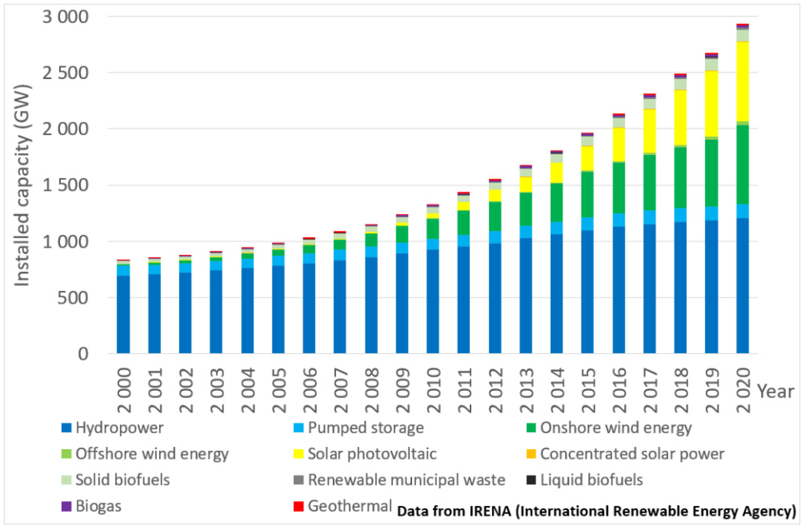
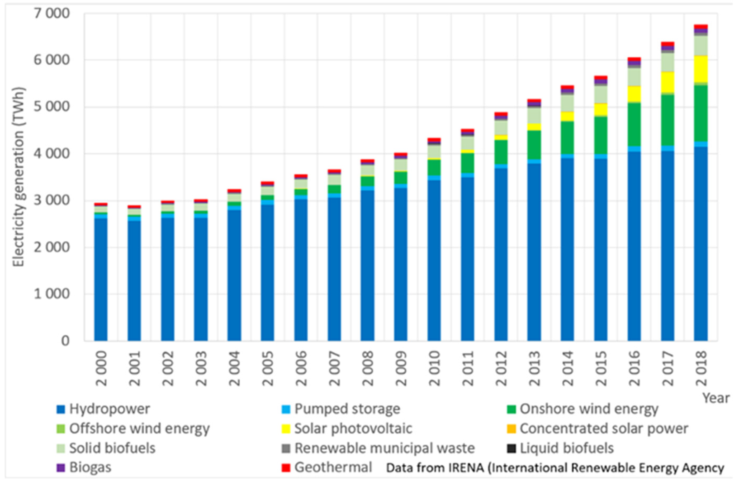
3. Renewable Energy Sources
4. Possibilities of Active Power Loss Reduction
- Decentralized Volt-Var Control—local volt/var controllers receive local information of the power system states.
- Centralized Volt-Var Control—central volt/var controllers receive all the information of the power system states.
- Hierarchical Volt-Var Control—controllers are organized in a hierarchical structure. All the controllers can receive partial or all information of the power system states [23].
- -
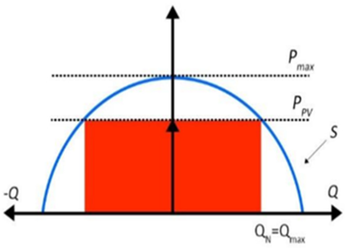
- Qmax and Qmin represent the reactive power range of the inverter;
- -
- umin and umax represent the boundaries in which there is no change in the reactive power; and
- -
- d is a parameter that specifies the linear decrease of the curve.
5. Optimization of Active Power Losses
- Classical optimization methods: these methods are based on strict mathematical techniques requiring calculation of the function gradient according to the regulated variables (for example, the projective gradient method, reduce gradient method, and sequential quadratic programming method).
- Alternative optimization methods: these methods are a combination of classical and stochastic methods. These methods use the properties of artificial intelligence (ability to retain knowledge, and to learn and solve problems), e.g., evolution algorithms (e.g., genetic algorithms, SOMA algorithm), expert systems, and methods using artificial neural networks [25].
5.1. Enumerative Method
5.2. Self-Organizing Migrating Algorithm (SOMA)
5.2.1. Self-Organizing Migrating Algorithm Parameters
- PathLength—is the length that the active element travels until it stops at a certain distance from the leader position. The usual setting range is between 1 and 3. The most commonly used value is 3, which means that in this case, the active element can move away until its path is tripled. When set to 1, the active element reaches exactly the same position as the leader [25]; thus, the minimum value should be greater than 1. This ensures the features always move away from the leader, and that the algorithm examined the environment and, after some time, found the best solution.
- Step—this parameter is used to sample the path of the active element [25].
- Population size—using this parameter, it is possible to set the size of the population, which is how many elements the population consists of. Within the population, it is recommended that the minimum number is set to a value of 10, and the maximum value is defined by the problem solver [25].
- Migration—is the first termination parameter. This parameter determines how many times it is possible to change the location of elements in the population It is recommended that its minimum value is set to 10, and the maximum value is not defined [25].
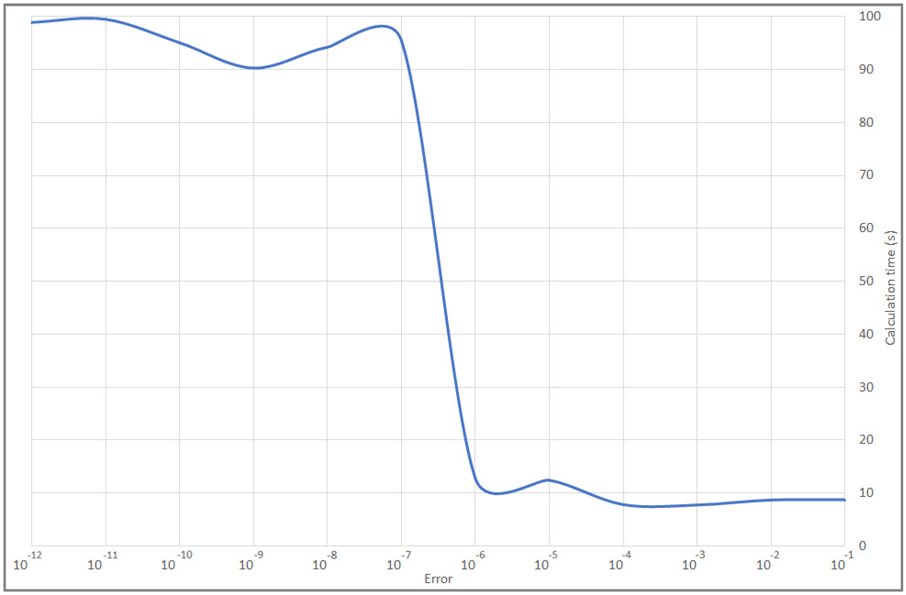
- Error—this is the second termination parameter. It is used to set when the algorithm should end its task with a certain accuracy. The algorithm detects the difference between the leading element and the worst element [25]. Setting the error parameter is a very important task as it can be used to determine how accurately the program will perform the calculations. The dependence of the calculation time on the error is shown in Figure 9.
5.2.2. SOMA Strategies
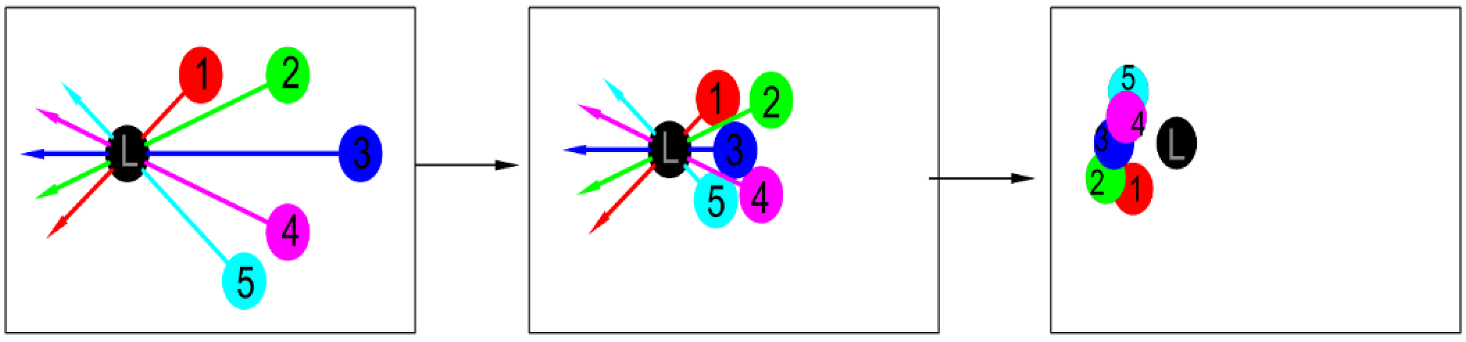
- AllToOne—AllToOne is the most commonly used SOMA strategy and has been used in this article. After creating an initial population, individuals choose each other, with the best becoming a leader (LEADER). During migration, other individuals begin to move toward the leader through the steps. The step value is defined in the SOMA parameters. If, when moving towards the leader, he finds a better purpose function value, then the individual stores the value in the memory and the individual returns to its original place. With such a procedure, the individual walks the entire length of his journey, and at the end, the individual goes to the best place that has been stored in his memory. This process is repeated by each individual, again choosing the best one who will be the new leader [25]. The whole process is repeated until at least one termination parameter is met. The number of migration cycles is achieved or the difference between the best and worst individuals is less than the “error” end parameter. The principle of the AllToOne strategy is shown in Figure 5.
- 2.
- AllToAll—the difference, compared to the previous strategy, is that after generating the initial population, individuals do not choose a leader for each other, and each individual is equal. All individuals move to all individuals (AllToAll) using a predefined step. When moving during the migration round, individuals observe whether their own actual values of the purpose function are better or worse compared to the starting positions. If they find a better one, they store the position in their memory and return to their initial position. After completing the entire journey, individuals update their positions based on their memory. In this case, the whole process is repeated until at least one termination parameter is met [25].The advantage of this strategy is a higher likelihood of finding a global extreme due to the migration of individuals. The disadvantage is the computational complexity, as it takes longer to find the best individual in the population. The principle of an all-to-all strategy is shown in Figure 6.
- 3.
- AllToAllAdaptive—the adaptive all-to-all strategy is almost the same as the previous one. The only difference is that in this case, if the individual finds a better value in his path, he will not only memorize the position, but the position will also become his new starting position. In the next migration round, the individual starts from this position. If he finds a better one while moving, he updates the position. The whole procedure is repeated until the end of the algorithm [25].
- 4.
- AllToAllRand—this strategy is similar to the first strategy (AllToAll), except in this case, the individuals move towards the leader. The difference is that leaders are not selected on the basis of the best purpose function but are selected at random from the population [25].
6. Simulated Network
Calculation of Steady Network Operation
7. Solving the Optimization Problem
7.1. Target Function
- The voltages in the nodes are ±10% of the voltage at the balance (in the first) node. The voltage at the balance node has a value of 23 kV; therefore, it is necessary to maintain a voltage of 20.7–25.3 kV.
- The value of the reactive power at the control nodes is 0–1 MVAr.
7.2. Research Limitations
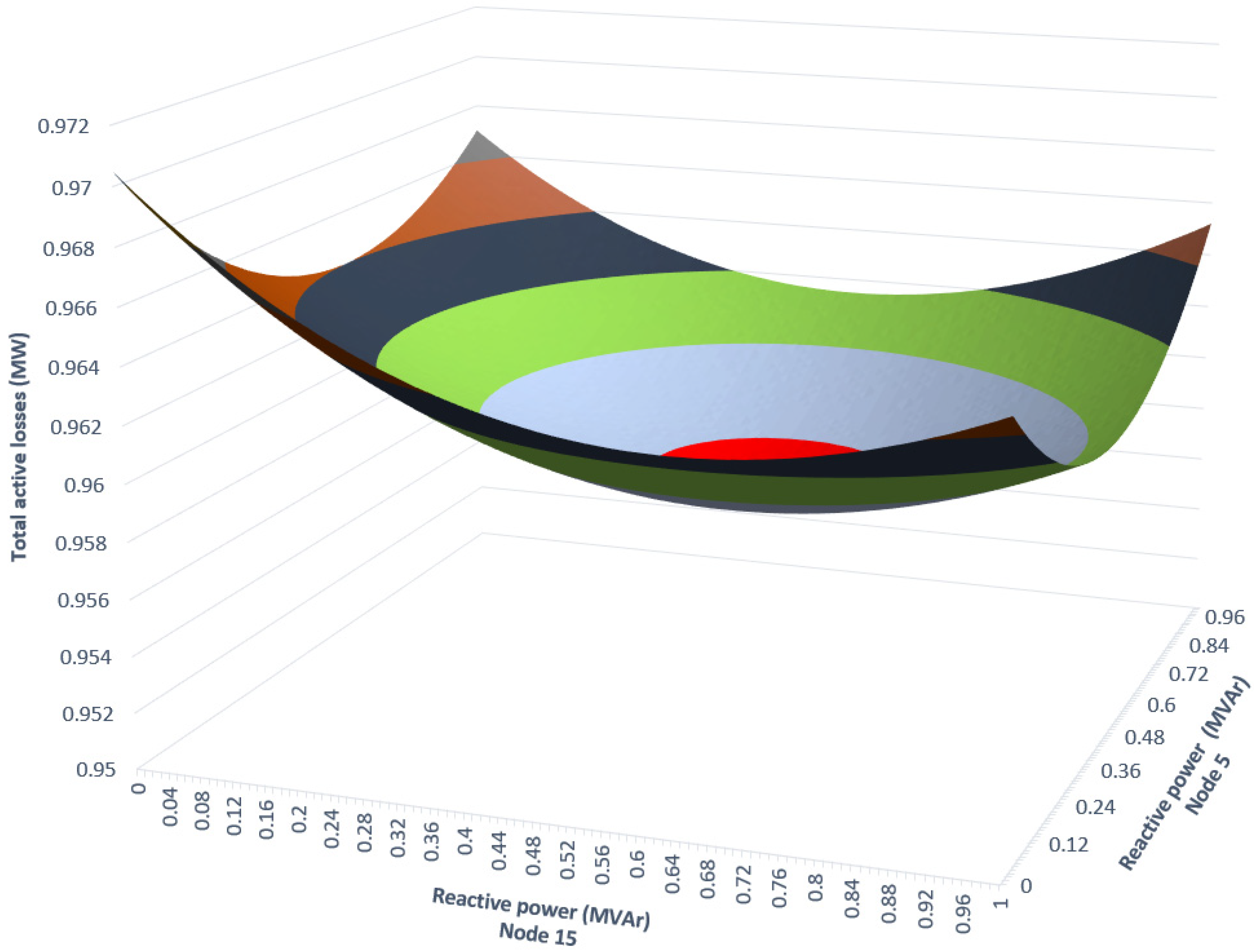
7.3. Solving the Optimization Problem by the Enumerative Method
7.4. Solving the Optimization Problem Using the SOMA Algorithm
8. Conclusions
Author Contributions
Funding
Conflicts of Interest
References
- Electricity Explained, How Electricity Is Delivered to Consumers. Electricity Is Delivered to Consumers through a Complex Network. Available online: https://www.eia.gov/energyexplained/electricity/delivery-to-consumers.php (accessed on 30 August 2021).
- Bouffard, F.; Kirschen, D.S. Centralised and distributed electricity systems. Energy Policy 2008, 36, 4504–4508. [Google Scholar] [CrossRef]
- Lost in Transmission: How Much Electricity Disappears between a Power Plant and Your Plug? Available online: http://insideenergy.org/2015/11/06/lost-in-transmission-how-much-electricity-disappears-between-a-power-plant-and-your-plug/ (accessed on 30 August 2020).
- Innovations and Decentralized Energy Markets? Available online: https://www.thecgo.org/research/innovations-and-decentralized-energy-markets/ (accessed on 1 September 2021).
- Zhou, Y.; Cao, S.; Hensen, J.L.; Lund, P.D. Energy integration and interaction between buildings and vehicles: A state-of-the-art review. Renew. Sustain. Energy Rev. 2019, 114, 109337. [Google Scholar] [CrossRef]
- Zhou, Y.; Cao, S. Coordinated multi-criteria framework for cycling aging-based battery storage management strategies for positive building—Vehicle system with renewable depreciation: Life-cycle based techno-economic feasibility study. Energy Convers. Manag. 2020, 226, 113473. [Google Scholar] [CrossRef]
- Internet of Things, Mikko Hyppönen: Smart Devices Are “IT Asbestos”. Available online: https://www.verdict.co.uk/mikko-hypponen-smart-devices-it-asbestos/ (accessed on 1 September 2021).
- The Smart Grid Could Hold the Keys to Electric Vehicles. Available online: https://innovationatwork.ieee.org/the-smart-grid-could-hold-the-keys-to-electric-vehicles/ (accessed on 27 August 2021).
- Smart Grids: What Is a Smart Electrical Grid—Electricity Networks in Evolution. Available online: https://www.i-scoop.eu/industry-4-0/smart-grids-electrical-grid/ (accessed on 25 August 2021).
- The Smart Grid. Available online: https://www.smartgrid.gov/the_smart_grid/smart_grid.html (accessed on 25 August 2021).
- European Smart Grids Technology Platform. Vision and Strategy for Europe’s Electricity Networks of the Future; European Smart Grids Technology Platform: Brussels, Belgium, 2006; pp. 1–38. [Google Scholar]
- 2020 Climate & Energy. Available online: https://ec.europa.eu/clima/policies/strategies/2020_en (accessed on 1 September 2021).
- Directive (EU) 2018/2001 of the European Parliament and of the Council of 11 December 2018 on the Promotion of the Use of Energy from Renewable Sources. Available online: https://eur-lex.europa.eu/legalcontent/EN/TXT/PDF/?uri=CELEX:32018L2001&from=SK (accessed on 1 September 2021).
- Solar Energy. Available online: https://www.irena.org/solar (accessed on 1 September 2021).
- Most Efficient Solar Panels: Solar Panel Cell Efficiency Explained. Available online: https://news.energysage.com/what-are-the-most-efficient-solar-panels-on-the-market/ (accessed on 25 August 2021).
- What Are the Best Solar Panels Available? Top Brands and Products Compared. Available online: https://news.energysage.com/best-solar-panels-complete-ranking/ (accessed on 25 August 2021).
- Dec, G.; Drałus, G.; Mazur, D.; Kwiatkowski, B. Forecasting Models of Daily Energy Generation by PV Panels Using Fuzzy Logic. Energies 2021, 14, 1676. [Google Scholar] [CrossRef]
- Dralus, G.; Mazur, D.; Gołębiowski, M.; Gołębiowski, L. One Day-Ahead Forecasting at Different Time Periods of Energy Production in Photovoltaic Systems Using Neural Networks. In Proceedings of the 2018 International Symposium on Electrical Machines (SME), Andrychow, Poland, 10–13 June 2018; pp. 1–5. [Google Scholar]
- Crisp, J.; Sharma, R.; George, T.; Hagaman, S.; Nguyen, H. Solar Inverter Interactions with DC Side. Available online: https://www.digsilent.com.au/publications/2018/papers/Solar%20inverter%20interactions%20with%20the%20DC%20side%20V3.pdf (accessed on 1 September 2021).
- Ivas, M.; Marušić, A.; Havelka, J.G.; Kuzle, I. P-Q capability chart analysis of multiinverter photovoltaic power plant connected to medium voltage grid. Int. J. Electr. Power Energy Syst. 2020, 116, 105521. [Google Scholar] [CrossRef]
- Ali, A.; Raisz, D.; Mahmoud, K. Sensitivity-based and optimization-based methods for mitigating voltage fluctuation and rise in the presence of PV and PHEVs. Int. Trans. Electr. Energy Syst. 2017, 27, e2456. [Google Scholar] [CrossRef]
- Golebiowski, L.; Gołębiowski, M.; Mazur, D. Inverters operation in rigid and autonomous grid. COMPEL—Int. J. Comput. Math. Electr. Electron. Eng. 2013, 32, 1345–1357. [Google Scholar] [CrossRef]
- Li, Q.; Zhang, Y.; Ji, T.; Lin, X.; Cai, Z. Volt/Var Control for Power Grids with Connections of Large-Scale Wind Farms: A Review. IEEE Access 2018, 6, 26675–26692. [Google Scholar] [CrossRef]
- Gubert, T.C.; Colet, A.; Casals, L.C.; Corchero, C.; Domínguez-García, J.L.; Sotomayor, A.A.d.; Martin, W.; Stauffer, Y.; Alet, P.-J. Adaptive Volt-Var Control Algorithm to Grid Strength and PV Inverter Characteristics. Sustainability 2021, 13, 4459. [Google Scholar] [CrossRef]
- Davendra, D.; Zelinka, I. Self-Organizing Migrating Algorithm, Methodology and Implementation. In New Optimization Techniques in Engineering; Springer International Publishing AG: Cham, Switzerland, 2016; ISBN 978-3-319-28159-9. Available online: https://link.springer.com/book/10.1007%2F978-3-319-28161-2 (accessed on 1 September 2021).


| Parameter | Type | Set Parameter |
|---|---|---|
| PathLength | Control | 1.20 |
| Step | Control | 0.05–0.10 |
| Population size | Control | 15 |
| Migration | Termination | 15 |
| Error | Termination | 10−6 |
| Branch | R (Ohm) | X (Ohm) | B (Siemens) | Branch | R (Ohm) | X (Ohm) | B (Siemens) |
|---|---|---|---|---|---|---|---|
| b.1 | 1.500 | 1.650 | 0.174 × 10⁻⁶ | b.11 | 1.453 | 1.001 | 9.640 × 10⁻⁶ |
| b.2 | 2.001 | 1.027 | 9.347 × 10⁻⁶ | b.12 | 1.518 | 0.779 | 7.091 × 10⁻⁶ |
| b.3 | 1.200 | 1.320 | 0.139 × 10⁻⁶ | b.13 | 1.449 | 0.743 | 6.768 × 10⁻⁶ |
| b.4 | 1.170 | 1.287 | 0.136 × 10⁻⁶ | b.14 | 1.202 | 0.828 | 7.978 × 10⁻⁶ |
| b.5 | 1.904 | 1.311 | 0.126 × 10⁻⁶ | b.15 | 0.960 | 1.056 | 0.111 × 10⁻⁶ |
| b.6 | 2.004 | 1.380 | 0.133 × 10⁻⁶ | b.16 | 1.260 | 1.386 | 0.146 × 10⁻⁶ |
| b.7 | 2.208 | 1.133 | 0.103 × 10⁻⁶ | b.17 | 1.932 | 0.991 | 9.024 × 10⁻⁶ |
| b.8 | 1.656 | 0.850 | 7.735 × 10⁻⁶ | b.18 | 1.350 | 1.485 | 0.157 × 10⁻⁶ |
| b.9 | 1.904 | 1.311 | 0.126 × 10⁻⁶ | b.19—TR2 | 6.292 | 28.350 | 0 |
| b.10 | 1.403 | 0.966 | 9.307 × 10⁻⁶ | b.20—TR3 | 6.292 | 28.350 | 0 |
| Node | P (MW) | Q (MVAr) | Node | P (MW) | Q (MVAr) |
|---|---|---|---|---|---|
| 1 | 0 | 0 | 11 | 0 | 0 |
| 2 | −2 | −0.3 | 12 | −1.3 | −0.1 |
| 3 | −1.2 | −0.15 | 13 | −0.9 | −0.15 |
| 4 | −1.6 | −0.2 | 14 | −1.5 | −0.1 |
| 5 | 0 | 0 | 15 | 0 | 0 |
| 6 | −1.2 | −0.1 | 16 | −2.5 | −0.4 |
| 7 | −0.9 | −0.1 | 17 | −2.9 | −0.4 |
| 8 | −1 | −0.05 | 18 | −3 | −0.5 |
| 9 | −1.4 | −0.25 | 19 | 1 | 0 |
| 10 | −0.1 | −0.05 | 20 | 1 | 0 |
| Node | Voltage [kV] | Branch | Active Power Losses [MW] | Reactive Power Losses [MVAr] |
|---|---|---|---|---|
| 1 | 23.000 | b.1 | 0.196 | 0.215 |
| 2 | 22.362 | b.2 | 0.006 | 0.003 |
| 3 | 22.248 | b.3 | 0.056 | 0.062 |
| 4 | 22.056 | b.4 | 0.024 | 0.027 |
| 5 | 21.855 | b.5 | 0.067 | 0.046 |
| 6 | 21.468 | b.6 | 0.050 | 0.034 |
| 7 | 21.127 | b.7 | 0.005 | 0.003 |
| 8 | 21.020 | b.8 | 0.008 | 0.004 |
| 9 | 21.007 | b.9 | 0.001 | 0.001 |
| 10 | 21.519 | b.10 | 0.003 | 0.002 |
| 11 | 21.580 | b.11 | 0.000 | 0.000 |
| 12 | 21.503 | b.12 | 0.020 | 0.010 |
| 13 | 21.322 | b.13 | 0.007 | 0.004 |
| 14 | 21.216 | b.14 | 0.031 | 0.021 |
| 15 | 21.712 | b.15 | 0.013 | 0.014 |
| 16 | 21.847 | b.16 | 0.067 | 0.074 |
| 17 | 22.195 | b.17 | 0.037 | 0.019 |
| 18 | 21.908 | b.18 | 0.340 | 0.374 |
| 19 | 22.102 | b.19 | 0.013 | 0.058 |
| 20 | 21.830 | b.20 | 0.013 | 0.059 |
| Total losses | 0.971 | 0.993 |
| Node | Voltage [kV] | Branch | Active Power Losses [MW] | Reactive Power Losses [MVAr] |
|---|---|---|---|---|
| 1 | 23.000 | b.1 | 0.192 | 0.211 |
| 2 | 22.401 | b.2 | 0.006 | 0.003 |
| 3 | 22.287 | b.3 | 0.055 | 0.060 |
| 4 | 22.127 | b.4 | 0.023 | 0.025 |
| 5 | 21.956 | b.5 | 0.067 | 0.046 |
| 6 | 21.571 | b.6 | 0.049 | 0.034 |
| 7 | 21.232 | b.7 | 0.005 | 0.003 |
| 8 | 21.125 | b.8 | 0.008 | 0.004 |
| 9 | 21.112 | b.9 | 0.001 | 0.001 |
| 10 | 21.622 | b.10 | 0.003 | 0.002 |
| 11 | 21.683 | b.11 | 0.000 | 0.000 |
| 12 | 21.606 | b.12 | 0.019 | 0.010 |
| 13 | 21.426 | b.13 | 0.007 | 0.004 |
| 14 | 21.321 | b.14 | 0.030 | 0.021 |
| 15 | 21.814 | b.15 | 0.012 | 0.013 |
| 16 | 21.920 | b.16 | 0.065 | 0.071 |
| 17 | 22.233 | b.17 | 0.037 | 0.019 |
| 18 | 21.947 | b.18 | 0.334 | 0.367 |
| 19 | 22.849 | b.19 | 0.016 | 0.071 |
| 20 | 21.931 | b.20 | 0.013 | 0.059 |
| Total losses | 0.958 | 0.998 | ||
| Calculation time [s]: | 628.77 | Ideal reactive power according to the calculation [MVAr] | ||
| Number of calculated combinations | 10,000 | Node 5 | 0.52 | |
| Node 15 | 0.58 | |||
| Node | Voltage [kV] | Branch | Active Power Losses [MW] | Reactive Power Losses [MVAr] |
|---|---|---|---|---|
| 1 | 23.000 | b.1 | 0.192 | 0.211 |
| 2 | 22.402 | b.2 | 0.006 | 0.003 |
| 3 | 22.287 | b.3 | 0.055 | 0.060 |
| 4 | 22.128 | b.4 | 0.023 | 0.025 |
| 5 | 21.959 | b.5 | 0.067 | 0.046 |
| 6 | 21.573 | b.6 | 0.049 | 0.034 |
| 7 | 21.234 | b.7 | 0.005 | 0.003 |
| 8 | 21.127 | b.8 | 0.008 | 0.004 |
| 9 | 21.114 | b.9 | 0.001 | 0.001 |
| 10 | 21.623 | b.10 | 0.003 | 0.002 |
| 11 | 21.684 | b.11 | 0.000 | 0.000 |
| 12 | 21.606 | b.12 | 0.019 | 0.010 |
| 13 | 21.426 | b.13 | 0.007 | 0.004 |
| 14 | 21.321 | b.14 | 0.030 | 0.021 |
| 15 | 21.813 | b.15 | 0.012 | 0.013 |
| 16 | 21.921 | b.16 | 0.065 | 0.071 |
| 17 | 22.233 | b.17 | 0.037 | 0.019 |
| 18 | 21.946 | b.18 | 0.333 | 0.367 |
| 19 | 22.894 | b.19 | 0.016 | 0.071 |
| 20 | 21.932 | b.20 | 0.013 | 0.059 |
| Total losses | 0.958 | 0.998 | ||
| Ideal reactive power according to the calculation [MVAr] | 0.555 | |||
| Calculation time [s]: | 8.507 | |||
Publisher’s Note: MDPI stays neutral with regard to jurisdictional claims in published maps and institutional affiliations. |
© 2022 by the authors. Licensee MDPI, Basel, Switzerland. This article is an open access article distributed under the terms and conditions of the Creative Commons Attribution (CC BY) license (https://creativecommons.org/licenses/by/4.0/).
Share and Cite
Pál, D.; Beňa, Ľ.; Kolcun, M.; Čonka, Z. Optimization of Active Power Losses in Smart Grids Using Photovoltaic Power Plants. Energies 2022, 15, 739. https://doi.org/10.3390/en15030739
Pál D, Beňa Ľ, Kolcun M, Čonka Z. Optimization of Active Power Losses in Smart Grids Using Photovoltaic Power Plants. Energies. 2022; 15(3):739. https://doi.org/10.3390/en15030739
Chicago/Turabian StylePál, Daniel, Ľubomír Beňa, Michal Kolcun, and Zsolt Čonka. 2022. "Optimization of Active Power Losses in Smart Grids Using Photovoltaic Power Plants" Energies 15, no. 3: 739. https://doi.org/10.3390/en15030739
APA StylePál, D., Beňa, Ľ., Kolcun, M., & Čonka, Z. (2022). Optimization of Active Power Losses in Smart Grids Using Photovoltaic Power Plants. Energies, 15(3), 739. https://doi.org/10.3390/en15030739