1. Introduction
The rapid development of industrialization has led to a sharp increase in carbon dioxide emissions in various countries, which has posed a serious threat to the earth’s life system. In fact, China has become the largest CO
2 emitter since 2009 [
1]. In order to actively respond to the impact of global climate change on economic development, environment and public health, countries around the world have advocated reducing carbon dioxide and greenhouse gas emissions in the form of the global Paris Agreement in 2015, and have set the goal of achieving net zero emissions in the second half of this century. At the general debate of the United Nations General Assembly in 2020, China said that it would adopt more powerful policies and measures and take the initiative to put forward a major international commitment to “strive to peak carbon dioxide emissions by 2030 and strive to achieve carbon neutrality by 2060”. The “carbon peak” goal means that China will peak CO
2 emissions by 2030 or earlier [
2]. For this purpose, China should increase the proportion of non-fossil energy in primary energy consumption to around 20% in 2030 and reduce unit GDP carbon by 60–65% more than that of 2005 [
3]. “Carbon neutralization” refers to the fact that countries, enterprises, products, activities or individuals offset their direct or indirect carbon dioxide emissions through energy conservation and emission reduction, so as to achieve relatively small emissions [
4]. The proposed “carbon peak” and “carbon neutralization” not only draws a grand blueprint for China’s low-carbon energy transformation and green economic development, but also shows China’s determination to implement the agreement commitments in order to achieve amicable and common development.
To achieve the goal of “carbon peak” and “carbon neutralization”, the core aim is to promote clean and low-carbon development of energy. The essence of this aim is to control and reduce the consumption of fossil energy, employ the optimal allocation of resources on a large scale, and improve the adaptability of clean energy and a clean energy system. Taking power generation as an example, in order to optimize the allocation of resources to a greater extent, it is necessary to save power resources to a greater extent on the basis of meeting power demand. Therefore, reasonable power load forecasting is of great significance for optimal allocation of resources. In this way, power generation can not only meet power demand, but avoid the waste of resources and the increase of consumption costs due to the large margin of power generation.
There has been some research on power load forecasting in the energy field, including power system load forecasting [
5], distributed photovoltaic load forecasting [
6], wind power load forecasting [
7], etc. Power load has a certain regularity and a certain randomness. Regularity is the basis of load forecasting, and randomness affects the accuracy of load forecasting. The purpose of load forecasting is to predict the future load trend by fully exploiting the regularity of historical load data. Therefore, it is of great significance to study the accuracy and regularity of the load forecasting model. In addition, climate factors also have an influence on the results of load forecasting.
The main research objectives of this paper are:
- (1)
Review the power load forecasting literature.
- (2)
Screen the main climate factors which influence the results of load forecasting by Pearson correlation coefficient screening and stepwise regression methods.
- (3)
Introduce the hybrid method to forecast the power load value.
- (4)
Put forward the load regularity index analysis method.
The research structure of this paper is organized as follows.
Section 2 is a relevant literature review regarding power load forecasting with multiple methods.
Section 3 introduces the screening and improved forecasting methods.
Section 4 focuses on case analysis. Firstly, climate factors affecting load forecasting are screened by the regression model and correlation test. Then an IPSO-Elman neural network algorithm is proposed to accurately predict the power load. Climate factors are introduced to compare and analyze their influence on the load forecasting results, and the rationality and effectiveness of the method is verified by comparing with the actual load value. Finally, the accuracy of load prediction is analyzed and compared by the cosine distance and error method, and it is proved that load regularity also affects the accuracy of load prediction. The conclusion of this paper is given in the final section.
2. Literature Review
At present, many scholars have carried out research on power load forecasting, including medium and long term power load forecasting and short term power load forecasting. Li and Jiang (2012) studied the factors affecting medium and long term power load and analyzed empirically medium and long term power load forecasting in the northeast of China [
8]. Xuan et al. (2017) constructed screening technique using the load forecasting model and the variable weight combination forecast method of medium and long term power system load forecasting [
9]. Wang et al. (2020) proposed a mid–long-term load forecasting method related to electricity market reform based on an improved SVR algorithm [
10]. Ji et al. (2018) used the load forecasting method of PSO to predict the load in the Weibei area [
11]. Zhang et al. (2018) proposed a novel load forecasting approach based on spatial–temporal feature clustering and extracted the temporal regular load pattern [
12].
There are also many short-term load forecasting studies. Javed et al. (2021) gave a comprehensive overview of modern linear and nonlinear parameter modeling techniques for short-term power load prediction considering time and climate factors, ensuring stable and reliable power system operation by mitigating non-linearities in power load data, and proved the effectiveness of the model by case analysis [
13]. Bin et al. (2014) established a short-term load forecasting model based on BP neural network theory taking full account of the relationship between the daily load and weather factors [
14]. Liu et al. (2016) built a power system short-term load forecasting model based on the support vector machine to improve forecasting accuracy and timeliness [
15]. Rafi et al. (2021) proposed a new approach for short-term load forecasting based on the integration of the convolutional neural network (CNN) and long short-term memory (LSTM) network [
16]. Xiao et al. (2017) used the singular spectrum analysis (SSA) with modified wavelet neural network (WNN) for all short-term load forecasting, short-term wind speed forecasting and short-term electricity price forecasting [
17]. Pei et al. (2020) proposed a hybrid feature selection method and applied an Improved Long Short-Term Memory network (ILSTM) to predict multi-step ahead load [
18].
In addition, many scholars have researched electricity demand. Shah et al. (2019) studied the effect of annual component estimation on one-day-ahead out-of-sample electrical prediction in advance by comparing different modeling techniques for electricity demand forecasting [
19]. Hirose et al. (2020) studied short-term power demand forecasting in a small-scale area considering event information in order to obtain high forecasting accuracy [
20]. Vilar et al. (2012) forecast electricity demand and electricity price based on nonparametric regression techniques with functional explanatory data and a semi-functional partial linear model and compared this with the naïve method and ARIMA forecasts [
21]. In order to extract complex irregular energy patterns and selectively learn temporal and spatial features in order to reduce the translation variance between energy attributes, Bu and Cho (2020) proposed a deep learning model based on a multi-attentional convolutional recurrent neural network to predict residential energy consumption [
22].
There are many methods for load forecasting, and scholars have adopted a variety. Cui et al. (2020) established the LSTM prediction model for load prediction to obtain more accurate power load prediction results according to the time series rule of power load [
23]. Tian and Yao (2015) improved the subspace method by introducing the feedback factor and the forgetting factor, and then optimized the values of these factors by PSO algorithm to improve prediction accuracy [
24]. Xu et al. (2018) proposed a method calling for corresponding data by accepting the load forecast request from the client, and performed the load forecasting on the big data by improving the gray model of the chaos genetic algorithm (CGA) [
25]. Elgarhy et al. (2017) presented an approach for short-term load forecasting using the artificial neural network technique, which utilized the historical hourly load data for accurate estimation of loads [
26]. Liu et al. (2018) put forward a short-term power load forecasting method according to the problems of high computational cost and over-fitting in traditional forecasting methods based on the combination of clustering with the eXtreme Gradient Boosting algorithm [
27].
Load forecasting is not only affected by internal factors of power system and forecasting methods, but also by many climate factors. However, the influence of climate factors on load prediction results is generally not considered in the above literature. This paper makes a more accurate prediction of power load on the basis of full consideration of the influence of climate factors.
The literature above selected some improved algorithms for load forecasting, but did not make a more in-depth analysis of forecasting accuracy on the basis of considering climate factors. This paper presents an improved IPSO-Elman neural network algorithm for more accurate load forecasting. In addition, the influence of climate factors on load forecasting results was compared and analyzed to prove the rationality of this improved method.
3. Method
In order to carry out load forecasting more accurately based on the screening of climate factors, this paper compares and analyzes the impact of climate factors on load forecasting, and then puts forward the method for screening climate factors and improving load forecasting.
3.1. Pearson Correlation Coefficient Screening Method and Stepwise Regression Method
In order to reasonably select climate variables for load forecasting, two methods are adopted to screen and verify each other, namely the Pearson correlation coefficient method and Stepwise regression method. The Pearson correlation coefficient can fairly accurately reflect the degree of linear correlation between two variables [
28].
Stepwise regression has been extensively used for determining the most influential variables in the linear regression model, adopting the method of advancing and retreating [
29].
Firstly, for variables outside the model, these can enter the model as long as they can also provide significant explanatory information. For variables that are already internal, as long as their partial F test cannot pass, they may be deleted from the model.
Secondly, the independent variables in the model are tested. The linear regression equation between the dependent variable and each independent variable is found and the variable with the largest value selected into the model. Then, the bias test is carried out for the remaining variables outside the model. Among the variables that pass the bias test, the one with the largest value is selected to enter the model. After adding variables to the model each time, the bias test is conducted for each variable in the model. If these all pass, new variables continue to be selected from outside the model. If not, the variables are eliminated and re-screened. Finally, the above steps are repeated until all variables outside the model fail to pass the bias test, then the algorithm terminates. In order to avoid the circulation of variables in and out, the critical value of the rejection domain of bias test is generally .
3.2. Improved Elman Neural Network Forecasting Model Based on PSO
3.2.1. Elman Neural Network Algorithm
At present, the BP neural network is the most widely used in the field of short-term load forecasting for power systems, but with the deepening of research, related problems are gradually exposed. In essence, the BP neural network uses a static feed-forward network to identify a dynamic system, i.e., it turns the dynamic time modeling problem into a static modeling problem, which leads to new problems. The Elman regression network is a typical dynamic neural network. Based on the basic structure of the BP artificial neural network, it has the function of mapping dynamic characteristics by storing internal states, so that the system has the ability to adapt to time-varying characteristics.
The Elman neural network is the typical local recursion delay feedback neural network, first proposed by Elman in 1990 [
30]. The Elman neural network is a kind of dynamic feedback network. On the basis of the hidden layer and output layer, a special connection unit is added, which is called the undertaking layer. The state space expression of its neural network mathematical model is:
where
and
represent node vectors of the hidden layer and undertaking layer, both of which have
.
represents the node vector of the hidden layer, and there are
in total.
represents the output node vector, which has
.
,
and
represent the weight matrix between the undertaking layer and hidden layer and the weight matrix between the layers, respectively.
and
represent the threshold vectors of the hidden layer and the output layer, respectively. Functions
and
represent the transfer function of neurons in the hidden layer and the output layer, respectively.
Elman neural network learning aims to minimize the sum of squares of the difference between the network output value and the expected output value, and the error function is:
where
and
represent the output value vector and the expected output value vector of the k-step system of the neural network, respectively.
3.2.2. Particle Swarm Optimization (PSO)
Particle Swarm Optimization (PSO) is a swarm intelligence technique proposed by Kennedy and Eberhart [
31]. Standard PSO is a stochastic search algorithm in multimodal search space, emerging from simulations of dynamic systems such as bird flocks and fish swarms [
32]. The idea of PSO is to obtain the optimal solution through the cooperation and sharing of information resources among different individuals in a group. Each particle in PSO represents a potential solution to the optimization problem and corresponds to a fitness value determined by a fitness function. Particle velocity determines the direction and distance of example movement, and the velocity is dynamically adjusted with the movement of itself and other particles, so as to realize individual optimization in solvable space. That is, all particles have a Fitness Value, which is determined by the optimized function, and its speed determines the distance and direction of particle movement. The particles know their current and best positions
so far, which can be regarded as the particles’ flight experience. In addition, the particles also know the best position
of all particles in the whole group so far. The best result in
is
, which can be regarded as the experience of particle companions.The particle determines the next step through its own experience and the best experience of its peers. The algorithm flow is as follows.
Step 1: Initialize the random velocity and position of the particle swarm.
Step 2: The adaptive value of each particle is calculated according to the objective function.
Step 3: Compare the fitness of each particle with the fitness of the best position experienced. If its adaptive value is better, it is the current best position.
Step 4: Compare the fitness of each particle with the fitness of the best position experienced by the whole world. If the adaptive value is better, it is regarded as the current global best position.
Step 5: Optimize the velocity and position of particles; the optimization strategy is as follows.
Step 6: If the constraint condition (large enough fitness value) is not met, return to step 2.
Step 7: Output the search results.
3.2.3. IPSO-Elman Algorithm
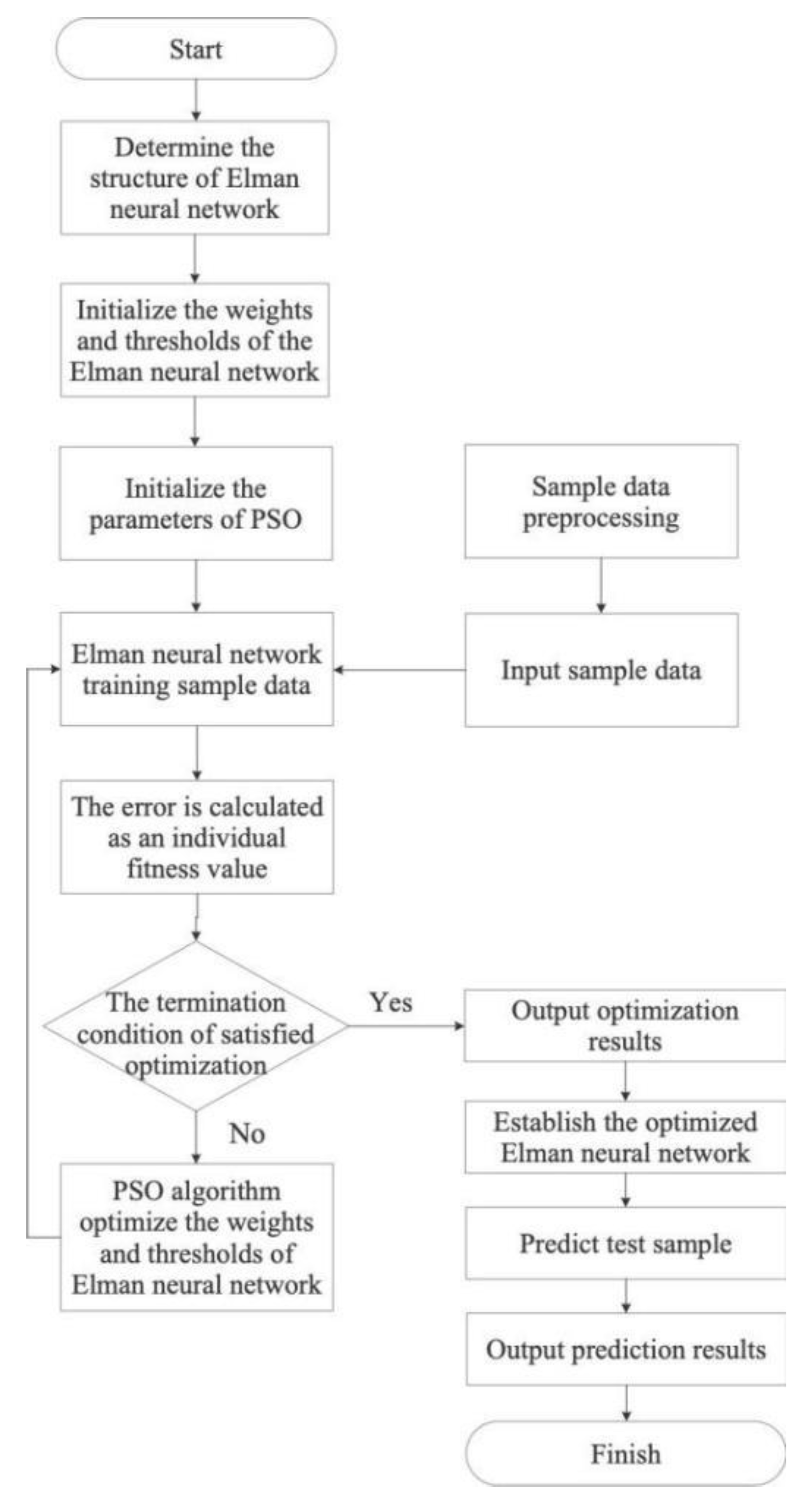
The Elman neural network trains the network according to the existing sample data and predicts the unknown with the known data. Its main advantage is that it can be adaptive to a large number of non-accurate and non-structural laws. However, the weight determination and selection of the Elman neural network structure have great influence on the prediction accuracy and training time. The Elman neural network uses a gradient descent algorithm to correct network thresholds and weights, but it is easy to fall into local minima. PSO has characteristics of efficient heuristic search, parallel computing and good global optimization ability.
This paper creatively uses an Elman neural network dynamic algorithm optimized by PSO to predict power load, which can not only adapt to a large number of nonlinear laws, but also learn independently after inputting climate data and historical load data. The Elman feedback neural network has outstanding advantages of dynamism and learning, which can not only reduce the number of input variables, but also effectively improve the prediction accuracy. On this basis, this paper applies PSO algorithm, which has characteristics of efficient heuristic search, parallel computing and good global optimization ability. While the Elman algorithm learns the data, the particle swarm optimization algorithm constantly looks for the optimal value from the initial weight or threshold of the data, which can better reflect the dynamic characteristics of the system and meet the needs of real-time changes in power load and weather. The optimal value was found from the initial weights and thresholds of the network, and the difference between the predicted value and the actual value was used as the fitness function of the particle swarm optimization algorithm. Then the IPSO-Elman (Improved PSO-Elman) network learning algorithm is constructed to the build load forecasting model. The optimization process of PSO reduces the prediction error and improves prediction accuracy. In this algorithm, firstly, according to the given input and output training samples, the number of nodes of the input layer, the implicit undertaking layer and the output layer of the Elman neural network is designed, the structure of the Elman neural network is determined, and the network parameters are initialized. The PSO algorithm is used to optimize network parameters. Finally, a new Elman neural network is established with optimized parameters to predict test samples. The prediction process of the IPSO-Elman neural network is shown in
Figure 1.
4. Case Study
In order to better verify the rationality of the proposed method, this paper selects the load data of two regions and continues the comparison of load forecasting. Based on the above analysis, it is known that the power load is also affected by climate factors. This section will specifically forecast the load under the influence of these climate factors.
4.1. Regression Analysis and Model Validation of Load Variables and Climate Factors
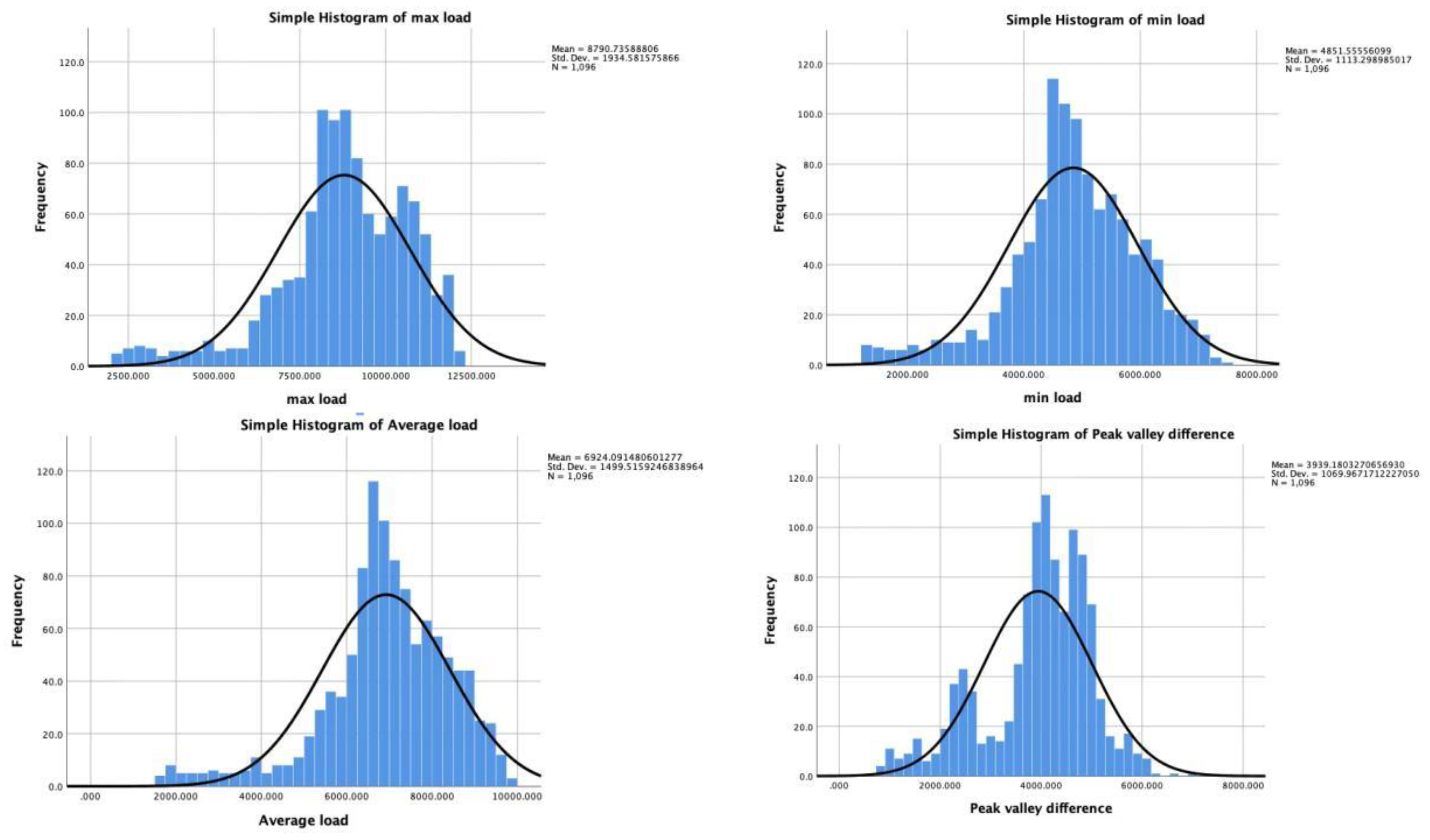
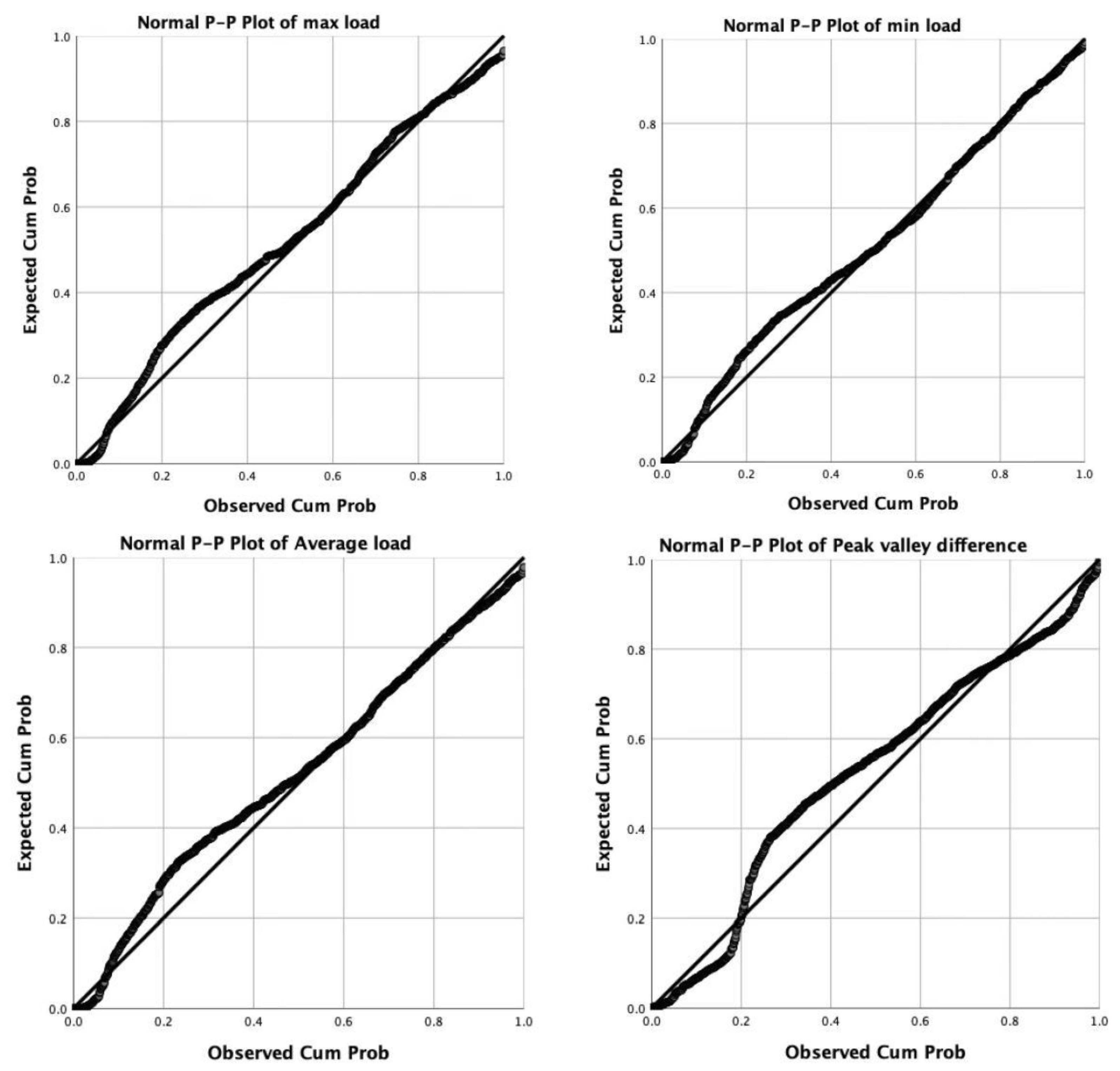
In order to better verify the distribution of maximum load, minimum load, average load and load peak–valley difference, SPSS was used to draw a histogram and P-P graph of these four indicators. A P-P graph is a scatter graph drawn according to the cumulative probability of variables corresponding to the cumulative probability of the specified theoretical distribution, which is used to intuitively detect whether the sample data conforms to the normal distribution. If the data being tested conforms to a normal distribution, the points representing the sample data should be roughly on the diagonal representing the theoretical distribution. The indicator histogram and P-P graph of Region 1 are shown in
Figure 2 and
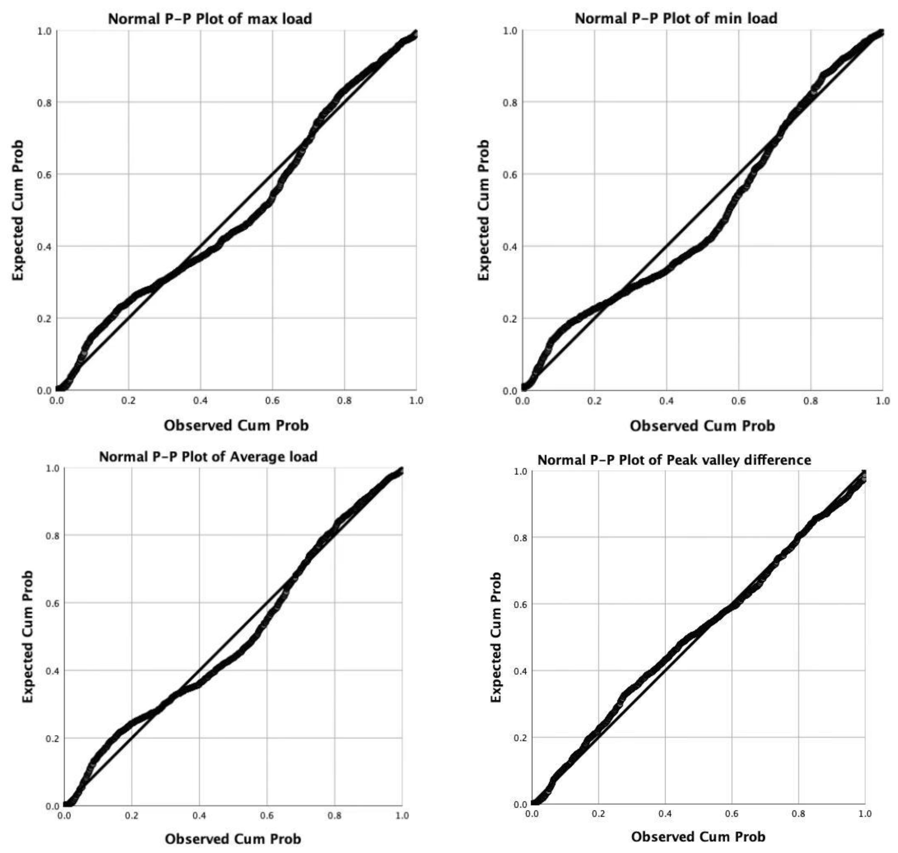
Figure 3. Indicator histogram and P-P graph for Region 2 are shown in
Figure 4 and
Figure 5.
From the distribution of the histograms, the distribution of each indicator has the following three characteristics. (1) Concentration, that is, the peak is in the center. (2) Symmetry, that is, the distribution curve is centered on the peak and is relatively symmetric. (3) Uniform variability. The distribution curve starts from the peak value and gradually decreases evenly to the left and right sides. These three characteristics are very close to a normal distribution. It can also be seen from the P-P diagrams that the scatter diagram of the cumulative probability of the theoretical distribution of the four indicators is very close to the diagonal distribution, which fully proves that the four indicators are close to the normal distribution.
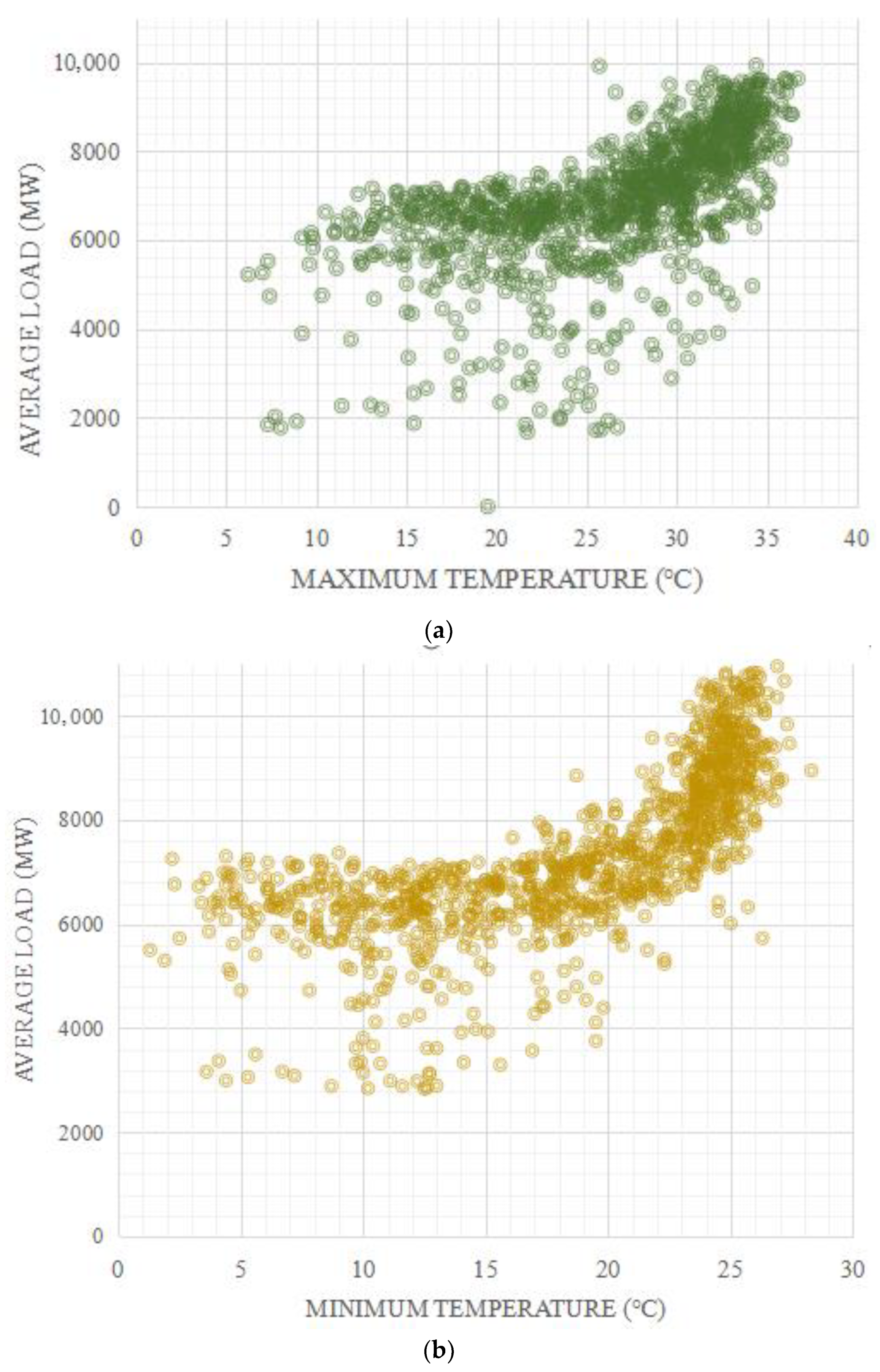
To find the relationship between daily maximum load, daily minimum load, daily average load and climate factors, it is necessary to conduct regression analysis. First, the regression model between load variables and meteorological variables is established, and the reliability of the regression model is tested. Secondly, the model error of the regression model is analyzed. Finally, the correlation test is used to test whether the impact of meteorological variables on load variables is significant, and the significance of impact is used as the evaluation standard to screen meteorological variables for load forecasting. We take the partial scatter plot results of the two regions as an example, as shown in
Figure 6.
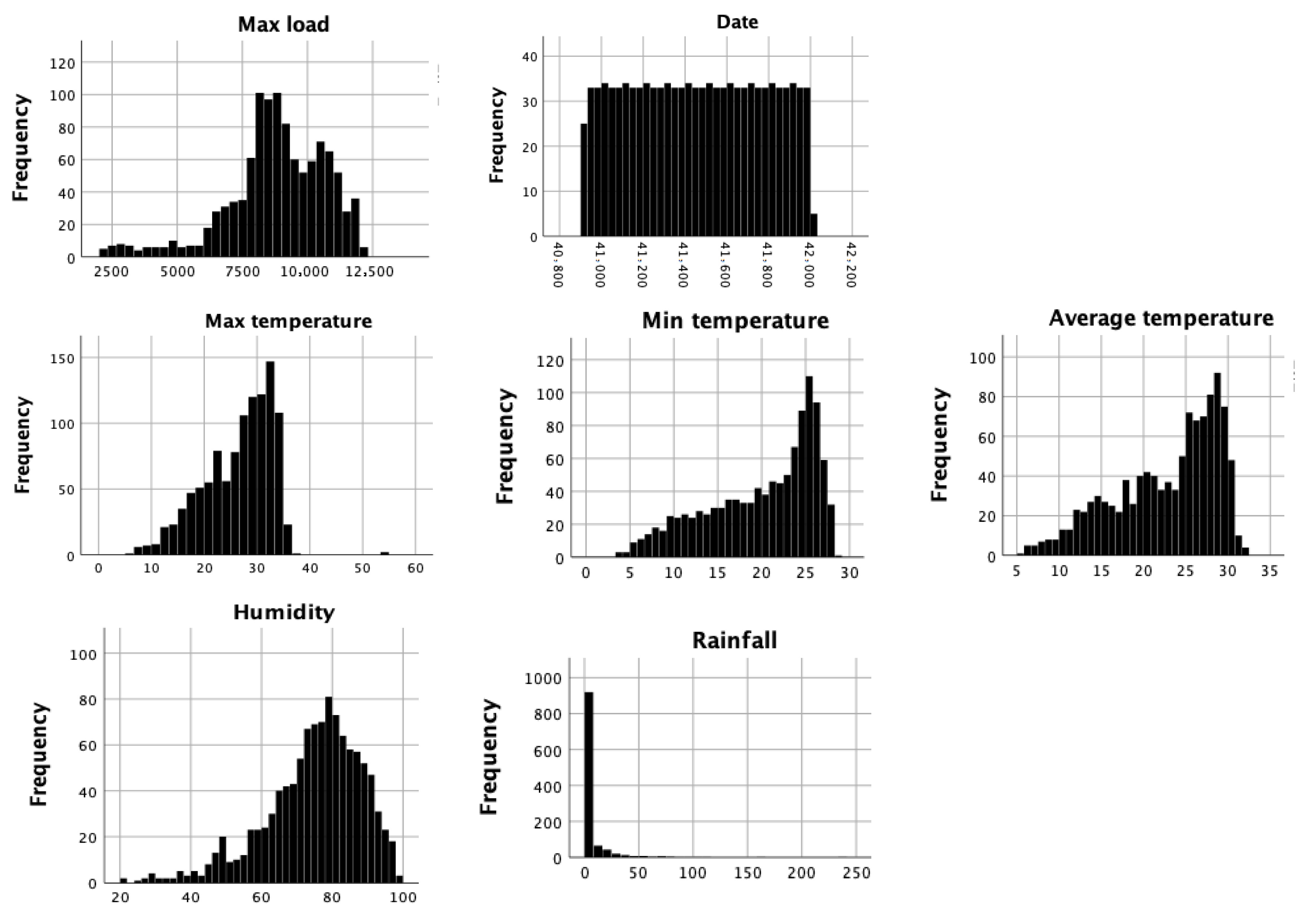
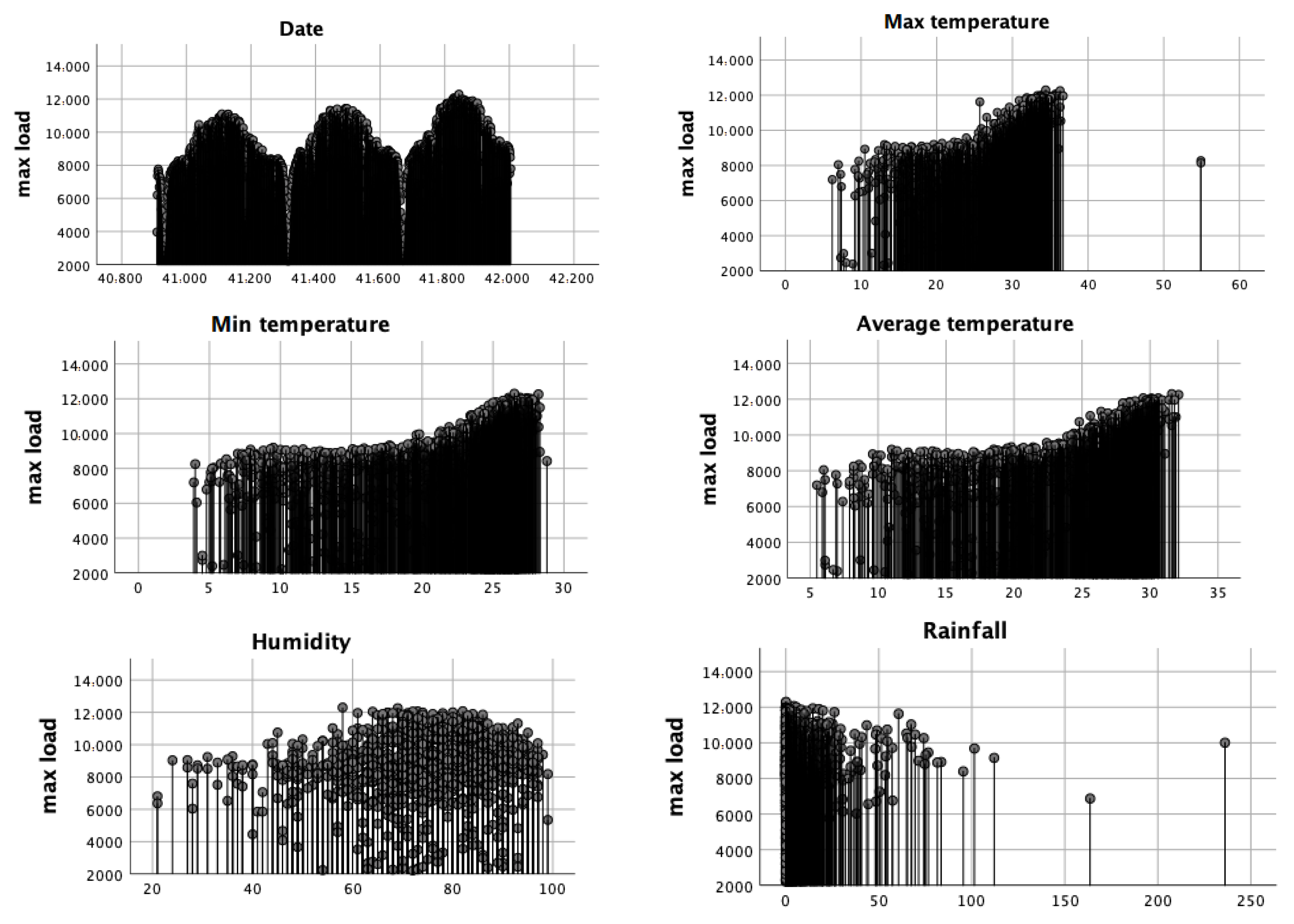
In addition, we conducted multivariate exploratory data analysis of multiple indicators of Region 1 as an example, as shown in
Figure 7 and
Figure 8. It can also be seen from the figure that each index has its own regularity, and the load data corresponding to climate factors also has a certain nonlinear relationship.
According to the distribution of the scatter diagram, it can be approximated that the daily maximum load , daily minimum load and daily mean load have a functional relationship with various meteorological variables (daily maximum temperature , daily minimum temperature , daily mean temperature , daily relative humidity and rainfall ).
4.1.1. Regression Model Error and Test of Region 1
SPSS software was used for multiple regression analysis of each variable, and the results of standardized regression analysis of Region 1 were as follows.
However, it can be seen that these data are based on time series and have a certain autocorrelation. In order to verify the existence of autocorrelation, we conducted a Durbin-Watson (DW) test. This is a common method to test sequence correlation. Through the DW autocorrelation test, the DW values of
,
and
regression functions are 0.676, 0.406 and 0.453, which also indicates that the regression model has a positive sequence correlation. Therefore, we use an iterative method to eliminate the autocorrelation error. According to
, the autocorrelation coefficients of the three regression functions in Region 1 are
,
,
. Then we get the processed regression function for Region 1 as follows.
The model error results can be calculated according to the standardization results, as shown in
Table 1. As can be seen, the values of
are close to 1, and the standard deviation error is within the acceptable range.
However, whether there is a linear relationship between load variables and climate variables as shown in the above model needs to be tested. Obviously, if all are small, the linear relationship between and is not obvious, so the original hypothesis can be written as .
When
is established,
defined by the decomposition formula satisfies:
Under significance level , there is an upper quantile of . If , then establish . Otherwise, reject the original hypothesis. In this paper, , the calculated of is greater than , so the original hypothesis is rejected. There is a linear relationship between load variables and climate variables as shown in the above model, and the model is established.
4.1.2. Regression Model Error and Test of Region 2
SPSS software was used for multiple regression analysis of each variable, and the results of the standardized regression analysis of Region 2 were as follows.
Through the DW autocorrelation test, the DW values of
,
and
regression functions are 0.466, 0.442 and 0.320, which also indicates that the regression model has a positive sequence correlation. In the same way, the autocorrelation coefficients of the three regression functions in Region 2 are
,
,
. Then we get the processed regression function for Region 2 as follows.
The model error results can be calculated according to the standardization results, as shown in
Table 2. As can be seen from
Table 2, the values of
are close to 1, and the standard deviation error is within the acceptable range.
Similar to the testing process in Region 1, , and the calculated of is greater than , so the original hypothesis is rejected. There is a linear relationship between load variables and climate variables as shown in the above model, and the model is established.
4.1.3. Correlation Test
Pearson correlation coefficient can quite accurately reflect the degree of linear correlation between two variables, so we conducted Pearson correlation analysis on the data to judge the correlation strength between climate variables and load variables. Pearson’s correlation coefficient is expressed as
The correlation coefficient is represented by
, which describes the degree of linear correlation between two variables. It is generally believed that the absolute value of correlation coefficient is highly correlated between 0.70 and 0.99, shows moderate correlation between 0.40 and 0.69, and low correlation between 0.10 and 0.39. The calculation results are shown in
Table 3.
It can be seen from
Table 3 that the correlation coefficients between
V8,
V9 and the load variables are 0.10–0.39, indicating low correlation. Therefore, we need to further use stepwise regression to screen variables. In this paper, the selected test level value is
and
. After stepwise regression analysis, we obtained the following results as shown in
Table 4.
As can be seen from
Table 4, most of the remaining variables after screening are concentrated on
,
and
. Therefore, we believe that the data for rainfall and relative humidity should not be selected, because the correlation coefficient between these two climate variables and load variables is small. Therefore, we choose daily maximum temperature, daily minimum temperature and daily average temperature as the basis of forecasting.
4.2. IPSO-Elman Algorithm Forecasting
4.2.1. Determine the Number of Neurons in IPSO-Elman Neural Network
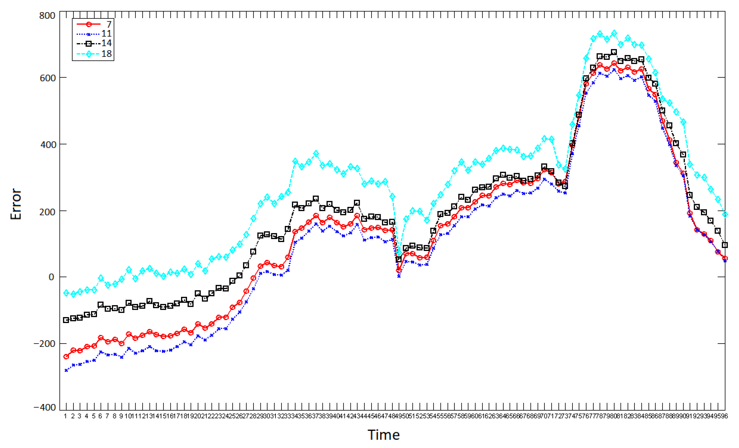
In order to determine the number of neurons, we first make a tentative forecast of the load value on 11 January 2021, and determine the final number of hidden layer neurons selected in the forecasting model by comparing the forecasting accuracy of neural network under different numbers of neurons.
According to the comparison in
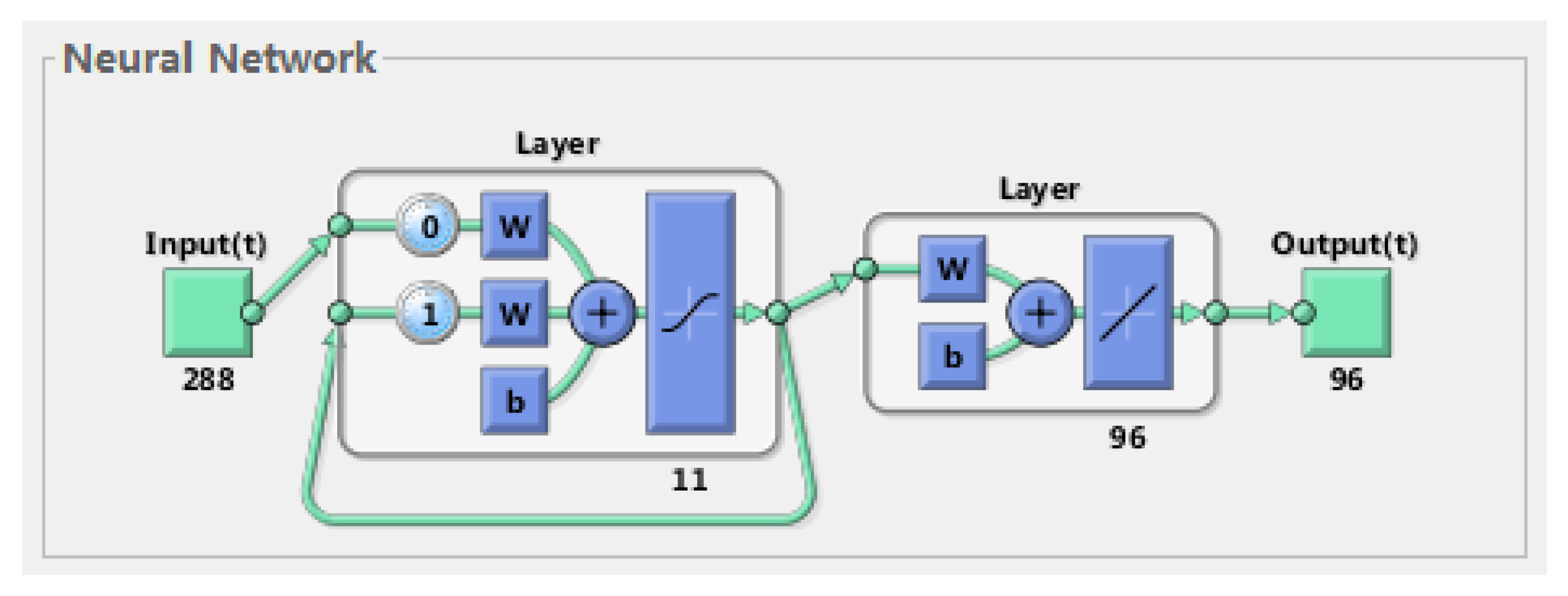
Figure 9, when the number of neurons in the hidden layer is 11, the error curve is the lowest and the neural network structure is the most reasonable. In view of this, the number of neurons in the hidden layer of our IPSO-Elman neural network was set as 11. At this point, the topology of the neural network is shown in
Figure 10.
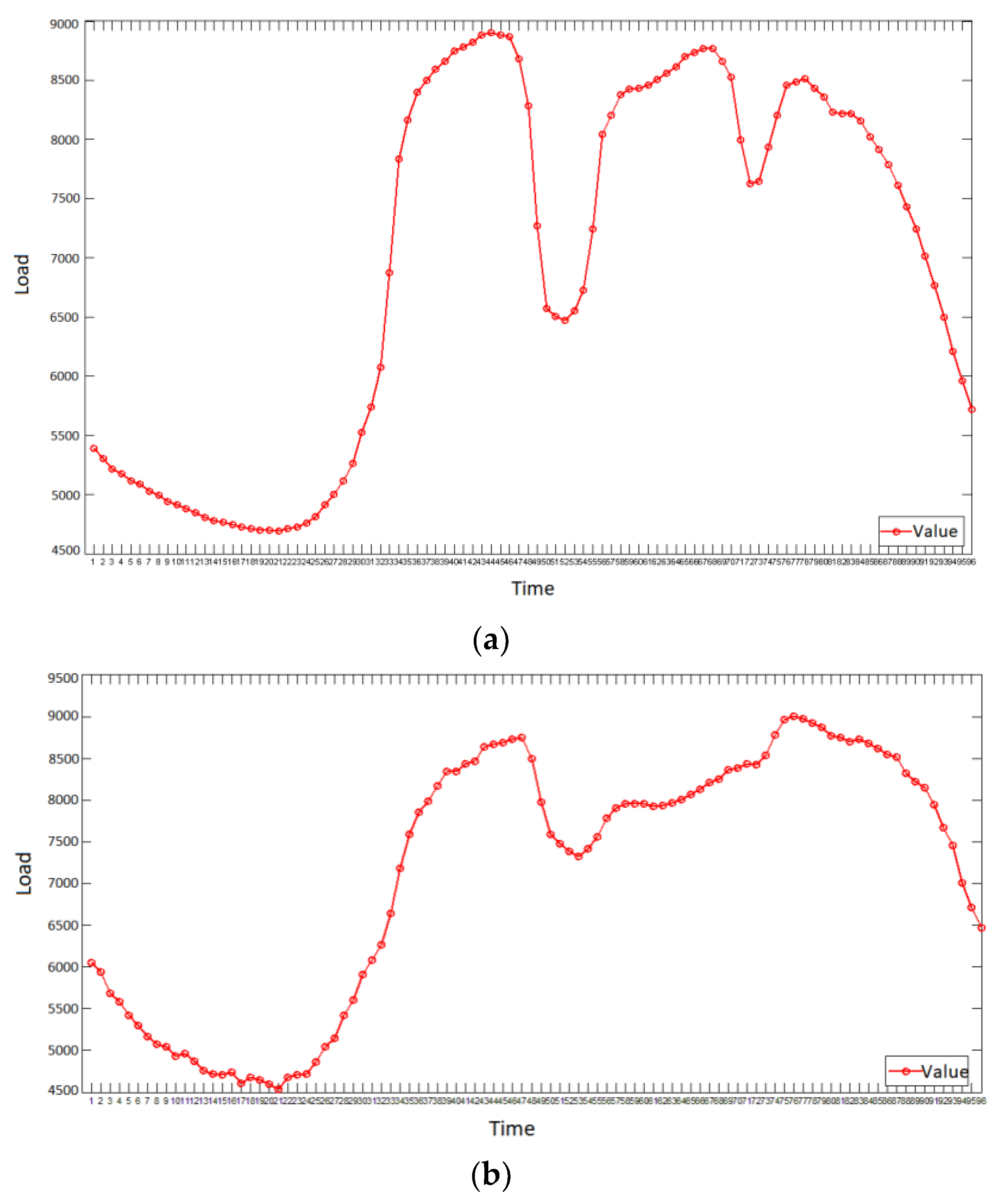
Figure 11 shows the load forecasting results of the IPSO-Elman neural network for 11 neurons in the hidden layer on 11 January 2021.
4.2.2. Select Input Quantity
The IPSO-Elman neural network forecasting method is used to forecast the power load of the two regions for 7 days from 11 January to 17 January 2021 (an interval of 15 min). Without considering climate factors, the input is only load data. In the process of forecasting, the rolling forecasting method of neural network is adopted. The input of network represents the load data of the three days before forecasting, and the output represents the load data of the forecast day. The specific rolling forecasting process is shown in
Table 5.
4.2.3. Forecast Results
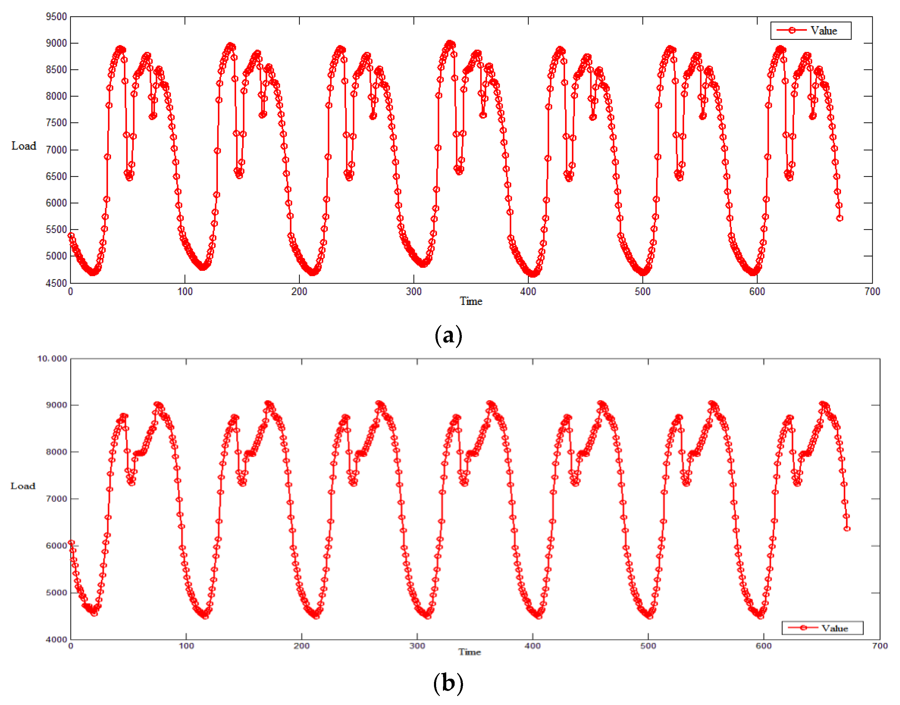
The load of Region 1 and Region 2 from 11 January 2021 to 17 January 2021 is predicted, and the forecasting results are shown in
Figure 12.
As can be seen from
Figure 12a, there are three peak points and two trough points in each fluctuation cycle. As can be seen from
Figure 12b, there are two peaks and two valleys in each fluctuation cycle. The load fluctuation of Region 1 and Region 2 shows obvious periodic characteristics, and the actual power system load also has a certain daily periodicity, which reflects the rationality of the prediction model in this paper to a certain extent.
4.3. IPSO-Elman Algorithm Forecasting Considering Climate Factors
In order to make a rigorous comparison between the prediction with and without climate factors, the IPSO-Elman neural network forecasting method is controlled by using the method of control variables, and the single historical data input is improved into a multi-input mode. The multiple inputs include historical load data and current climate data.
4.3.1. Construction of Forecasting Model Considering Climate Factors
In order to ensure the objectivity of forecasting to the maximum extent, this paper uses all climate data such as daily maximum temperature
V5, daily minimum temperature
V6, daily average temperature
V7, daily relative humidity
V8 and rainfall
V9 as the input of forecasting. The seven-day rolling forecast process considering climate factors is shown in
Table 6.
4.3.2. Forecasting Results and Analysis
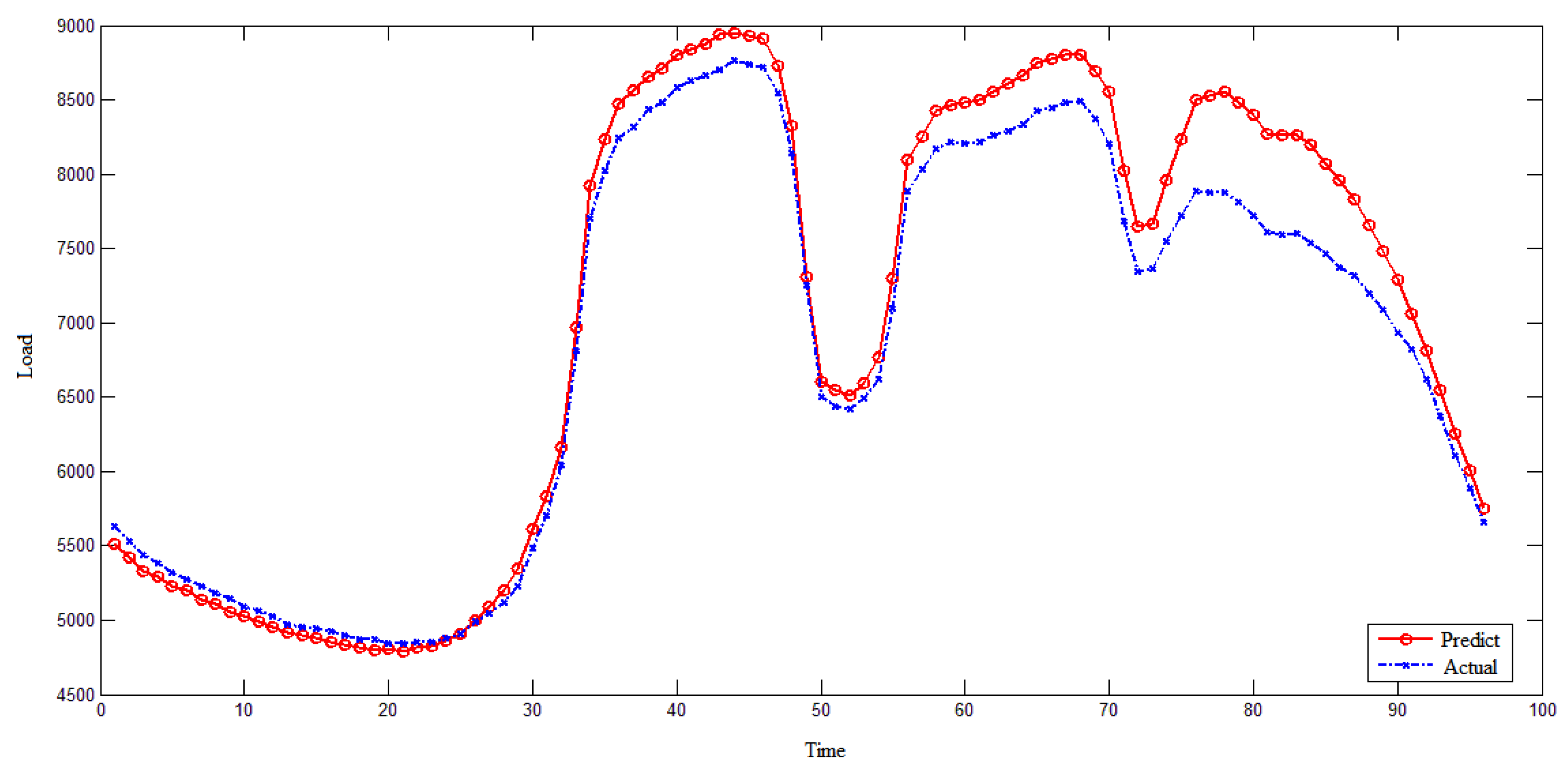
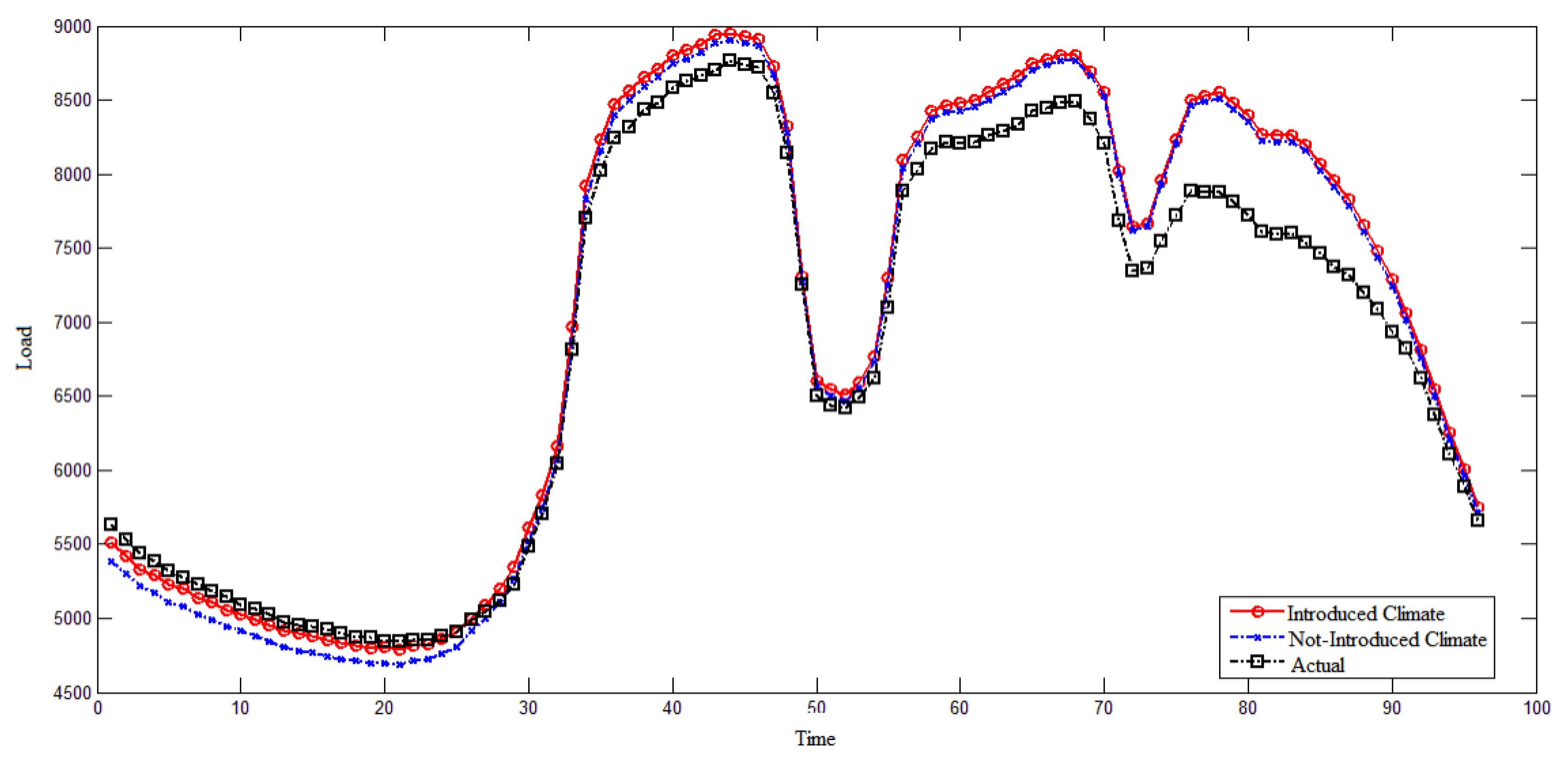
Firstly, the load forecasting results from 11 January to 17 January 2021 are shown in
Figure 13. In order to compare the forecast results with and without climate factors, the load condition on 10 January was predicted by using the data from 7 January to 9 January. Since the load data on 10 January is accurately known, it can be used as a standard reference. The load situation on 10 January was predicted (including and excluding climate factors), and compared with the standard data of the load on 10 January. The comparison results are shown in
Figure 14 and
Figure 15.
4.4. Discussion
4.4.1. Prediction Error Analysis
The prediction results show that the load situation of region 1 and region 2 presents obvious daily periodicity, and the actual power system load also has a certain daily periodicity, which indirectly verifies the reliability and precision assurance of our prediction model. However, whether taking climate into account can lead to better predictions needs to be proven.
As can be seen from
Figure 14 and
Figure 15, the two forecasting methods are very close to the actual value. In order to deeply compare the advantages and disadvantages of the two methods, the concept of cosine distance is introduced (Equation (8)). In this section, the cosine distance between the forecasting load curve with climate factors and the actual curve was calculated respectively, and the cosine distance between the forecasting load curve without climate factors and the actual curve was calculated separately. The calculation results are shown in
Table 7.
Through error analysis, we can see that the cosine distance of the two forecasting methods is very close to 1, which means that the forecasting results of these two methods are very close to the actual load situation. From the perspective of average error, the error of the model including climate factors is smaller, which means that the forecasting accuracy of the model is higher when the climate factors are included.
In addition, the average relative error
, root mean square error
and average relative error
of each model are calculated and compared to verify the effectiveness of the proposed method (
Table 8). According to the comparison in
Table 8, considering climate factors in load prediction can improve the prediction accuracy. The errors of the prediction model with climate factors are better than the prediction model without climate factors, which proves the effectiveness of the proposed method.
4.4.2. Load Regularity Analysis
Load variation has regularity and randomness: regularity is the basis of load forecasting, and randomness affects the accuracy of load forecasting. The task of load forecasting is to predict the future load trend by fully exploiting the regularity in the historical load data as much as possible. However, the random factors in load variation exist objectively, and the difference of load regularity in different regions and different periods will have a great influence on the load prediction results. Power load has strong periodicity, so it can be analyzed by using the time series frequency domain analysis method. The load time series to be analyzed is set as
, and Fourier decomposition performed to obtain:
where N is the length of load sequence. By the nature of Fourier decomposition, the resulting signals are orthogonal to each other. Thus, load
can be decomposed into components of angular frequency
. Through appropriate combination and according to the cyclical characteristics of load changes,
can be reconstructed as follows:
where
, whose period is 96, is the periodic component of the load that changes in 24 h, and
, whose period is
, is the periodic component of the load. These two components are load components that change according to a fixed period and can be extrapolated in the prediction.
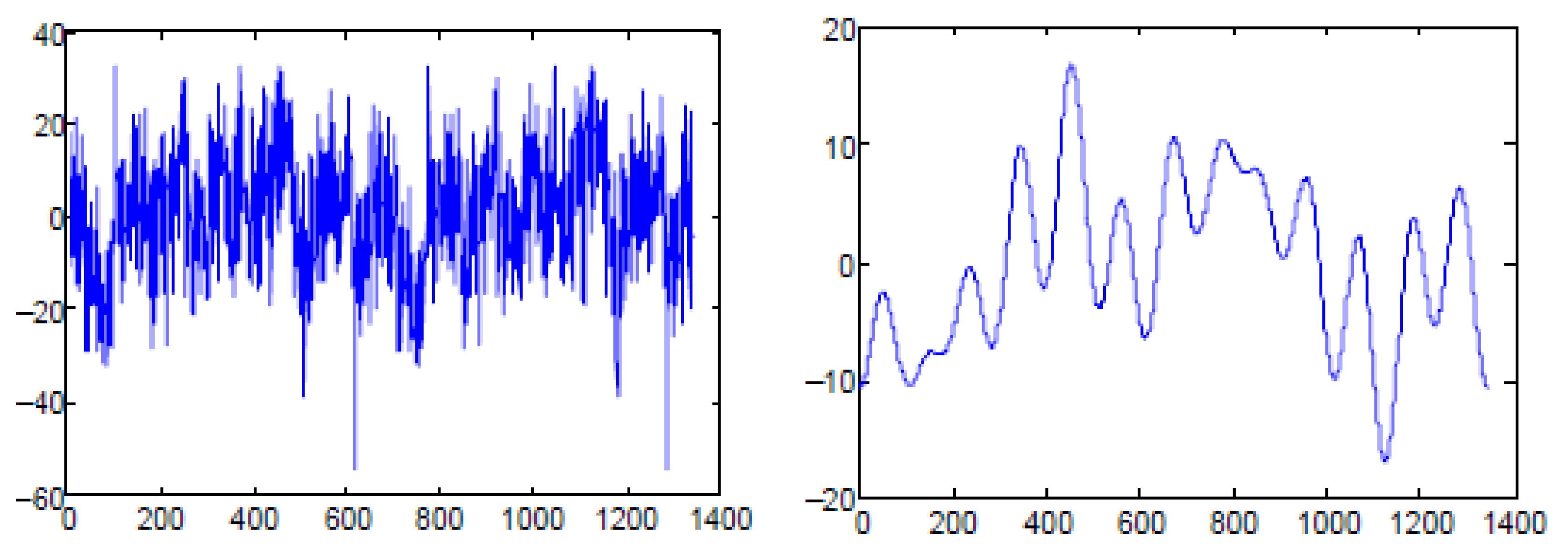
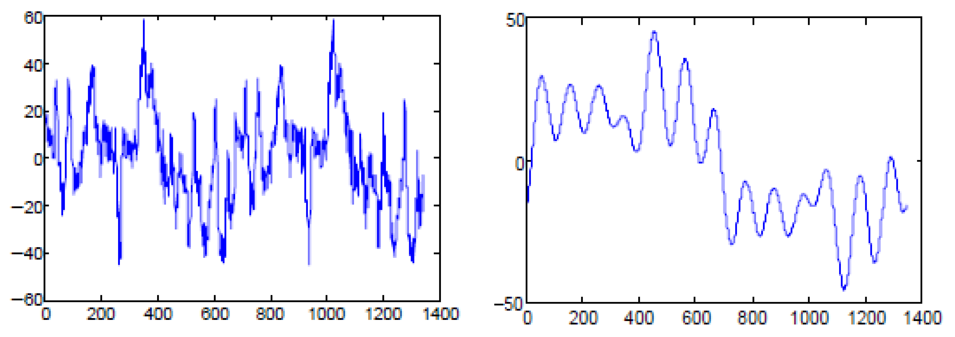
After removing , and the fixed components, the remaining components can be divided into and . is the sum of low-frequency components among the remaining components, reflecting the impact of slow variation-related factors such as meteorological factors on the load, while is the sum of high-frequency components among the remaining components, mainly reflecting the randomness of load changes.
Therefore, we introduce the stability index of historical load regularity. Stability shows the proportion of the load to the total load, which is easy to grasp. The proportion of high frequency component in the power load determines its stability. We can separate the high-frequency components in the time series to estimate the upper limit of stability of historical load, and the expression is as follows:
At the same time, the low-frequency component is generally related to climate factors. The minimum prediction ability of a load forecasting system is that it can accurately predict the parts of the power network load except low frequency and high frequency. The lower limit of stability of historical load is:
We take the period from 1 January 2020 to 14 January 2020 for frequency domain analysis and comparison. The following figures provide the comparison diagram of system load decomposition (See
Figure 16 and
Figure 17).
According to the result in
Table 9, the upper and lower limits of the estimated stability of region 1 are significantly lower than that of Region 2, which indicates that the proportion of historical load randomness factors in region 1 is higher than that in Region 1. Therefore, we believe that region 2 has better load regularity. At the same time, we know from the previous analysis that the distribution of the parameters of region 2 is closer to the normal distribution and the prediction model of Region 2 is slightly more accurate than that of Region 1.
In conclusion, we believe that there is a certain relationship between the distribution of parameter indexes and the regularity of load, and the accuracy of the prediction model is not only related to the prediction method but also to the regularity of historical load in the predicted region.
Despite the complexity of IPSO-Elman model, this paper applies it to power load prediction in a simple form. This method is very flexible in using historical point data for prediction, while new variables can be input in parameter or non-parameter form. Therefore, this method has good effectiveness.
5. Conclusions
In order to explore the influence of climate factors on load forecasting results, this paper proposed a power load forecasting model based on the IPSO-Elman algorithm. Firstly, the normal distribution of various indicators was verified by direct analysis of the histograms and P-P diagrams, and a multiple linear regression model between dependent variables and independent variables was built. The meteorological variables of load prediction were screened by Pearson correlation coefficient stepwise regression analysis. Secondly, the Elman neural network prediction model improved by particle swarm optimization is constructed. The prediction results show that the load conditions of region 1 and region 2 show obvious daily periodicity, and the actual power system load also has a certain daily periodicity, which indirectly verifies the reliability and precision assurance of the prediction model. Thirdly, in order to accurately compare the prediction with and without climate factors, the prediction model with a single type of historical data input is improved to a prediction model with parallel input of climate data and historical load data. Finally, the calculation of cosine distance and various error indexes proves that the error of the model is smaller and the prediction accuracy of the model is higher. In addition, by discriminating the regularity of load, it is proved that the accuracy of the prediction model is not only related to the forecasting method but also to the regularity of historical load.
There are also some shortcomings and limitations in this paper. There is a certain relationship between the weight of climate factors and the amount of relevant data. If the number of climate factors is small, the impact of climate factors on load forecasting results is not obvious. In addition, in the actual power system, there may be more factors affecting load. In the subsequent research, we will focus on exploring variables affecting load forecasting and study various methods, in order to find those that can adapt to different load prediction conditions.
Author Contributions
Conceptualization, J.L. and Y.Y.; methodology, Y.Y.; software, Y.Y.; validation, J.L. and Y.Y.; formal analysis, Y.Y.; investigation, Y.Y.; resources, J.L.; data curation, Y.Y.; writing—original draft preparation, J.L. and Y.Y.; writing—review and editing, J.L.; visualization, Y.Y.; supervision J.L.; project administration, J.L.; funding acquisition, J.L. All authors have read and agreed to the published version of the manuscript.
Funding
This research received no external funding.
Data Availability Statement
Conflicts of Interest
The authors declare that they have no known competing financial interests or personal relationships that could have appeared to influence the work reported in this paper.
References
- Wu, L.; Chen, Y.; Feylizadeh, M.R.; Liu, W. Estimation of China’s macro-carbon rebound effect: Method of integrating Data Envelopment Analysis production model and sequential Malmquist-Luenberger index. J. Clean. Prod. 2018, 198, 1431–1442. [Google Scholar] [CrossRef]
- Wu, L.; Zhu, Q. Impacts of the carbon emission trading system on China’s carbon emission peak: A new data-driven approach. Nat. Hazards 2021, 107, 2487–2515. [Google Scholar] [CrossRef]
- Dong, F.; Hua, Y.; Yu, B. Peak Carbon Emissions in China: Status, Key Factors and Countermeasures—A Literature Review. Sustainability 2018, 10, 2895. [Google Scholar] [CrossRef] [Green Version]
- Lu, W.; Li, Y.-S. Impact of the Paris Agreement on China’s Carbon Reduction and the Economy. Asian Stud. 2021, 24, 129–150. [Google Scholar] [CrossRef]
- Wang, Y.; Wu, L. Improving economic values of day-ahead load forecasts to real-time power system operations. IET Gener. Transm. Distrib. 2017, 11, 4238–4247. [Google Scholar] [CrossRef]
- Wang, Y.; Zhang, N.; Chen, Q.; Kirschen, D.S.; Li, P.; Xia, Q. Data-Driven Probabilistic Net Load Forecasting with High Penetration of Behind-the-Meter PV. IEEE Trans. Power Syst. 2017, 33, 3255–3264. [Google Scholar] [CrossRef]
- Sengar, S.; Liu, X. Ensemble approach for short term load forecasting in wind energy system using hybrid algorithm. J. Ambient Intell. Humaniz. Comput. 2020, 11, 5297–5314. [Google Scholar] [CrossRef]
- Li, J.; Jiang, Z.H. Study on Medium and Long Term Power Load Forecasting in Cold Regions. Appl. Mech. Mater. 2012, 170–173, 3472–3477. [Google Scholar] [CrossRef]
- Wenbo, X.; Jia, S.; Weidong, X.; Dawei, Y.; Zheng, L.; Jin, Z. The model combination method of power system load forecasting based on freshness availability index. In Proceedings of the 2017 2nd International Conference on Power and Renewable Energy (ICPRE), Chengdu, China, 20–23 September 2017; pp. 585–588. [Google Scholar] [CrossRef]
- Wang, W.; Dou, F.; Yu, X.; Liu, G.; Zhang, L.; Zhang, Q.; Xie, D. Load forecasting method based on SVR under electricity market reform. IOP Conf. Ser. Earth Environ. Sci. 2020, 467. [Google Scholar] [CrossRef]
- Ji, G.; Li, S.; Shi, Z.; Zhang, X.; Zhao, W. Regional Power Load Forecasting Based on PSOSVM. In Proceedings of the 2018 IEEE 4th Information Technology and Mechatronics Engineering Conference (ITOEC), Chongqing, China, 14–16 December 2018; pp. 1685–1688. [Google Scholar] [CrossRef]
- Zhang, W.; Mu, G.; Yan, G.; An, J. A power load forecast approach based on spatial-temporal clustering of load data. Concurr. Comput. Pract. Exp. 2017, 30, e4386. [Google Scholar] [CrossRef]
- Javed, U.; Ijaz, K.; Jawad, M.; Ansari, E.A.; Shabbir, N.; Kütt, L.; Husev, O. Exploratory Data Analysis Based Short-Term Electrical Load Forecasting: A Comprehensive Analysis. Energies 2021, 14, 5510. [Google Scholar] [CrossRef]
- Bin, H.; Zu, Y.X.; Zhang, C. A Forecasting Method of Short-Term Electric Power Load Based on BP Neural Network. Appl. Mech. Mater. 2014, 538, 247–250. [Google Scholar] [CrossRef]
- Liu, Q.; Huang, Z.Z.; Li, S. Research on power load forecasting based on support vector maching. J. Balkan Tribol. Assoc. 2016, 22, 151–159. [Google Scholar]
- Rafi, S.H.; Masood, N.A.; Deeba, S.R.; Hossain, E. A Short-Term Load Forecasting Method Using Integrated CNN and LSTM Network. IEEE Access 2021, 9, 32436–32448. [Google Scholar] [CrossRef]
- Xiao, L.; Shao, W.; Yu, M.; Ma, J.; Jin, C. Research and application of a hybrid wavelet neural network model with the improved cuckoo search algorithm for electrical power system forecasting. Appl. Energy 2017, 198, 203–222. [Google Scholar] [CrossRef]
- Pei, S.; Qin, H.; Yao, L.; Liu, Y.; Wang, C.; Zhou, J. Multi-Step Ahead Short-Term Load Forecasting Using Hybrid Feature Selection and Improved Long Short-Term Memory Network. Energies 2020, 13, 4121. [Google Scholar] [CrossRef]
- Shah, I.; Iftikhar, H.; Ali, S.; Wang, D. Short-Term Electricity Demand Forecasting Using ComponentsEstimation Technique. Energies 2019, 12, 2532. [Google Scholar] [CrossRef] [Green Version]
- Hirose, K.; Wada, K.; Hori, M.; Taniguchi, R.-I. Event Effects Estimation on Electricity Demand Forecasting. Energies 2020, 13, 5839. [Google Scholar] [CrossRef]
- Vilar, J.M.; Cao, R.; Aneiros, G. Forecasting next-day electricity demand and price using nonparametric functional methods. Int. J. Electr. Power Energy Syst. 2012, 39, 48–55. [Google Scholar] [CrossRef]
- Bu, S.-J.; Cho, S.-B. Time Series Forecasting with Multi-Headed Attention-Based Deep Learning for Residential Energy Consumption. Energies 2020, 13, 4722. [Google Scholar] [CrossRef]
- Cui, C.; He, M.; Di, F.; Lu, Y.; Dai, Y.; Lv, F. Research on Power Load Forecasting Method Based on LSTM Model. In Proceedings of the 2020 IEEE 5th Information Technology and Mechatronics Engineering Conference (ITOEC), Chongqing, China, 12–14 June 2020; pp. 1657–1660. [Google Scholar] [CrossRef]
- Huixin, T.; Jiaxin, Y.; Tian, H. A novel improved data-driven subspace algorithm for power load forecasting in iron and steel enterprise. In Proceedings of the 27th Chinese Control and Decision Conference (2015 CCDC), Qingdao, China, 23–25 May 2015; pp. 6421–6426. [Google Scholar] [CrossRef]
- Xu, M.; Huang, G.; Zhang, M.; Cui, P.; Wang, C. Load Forecasting Research Based on High Performance Intelligent Data Processing of Power Big Data. In Proceedings of the 2018 2nd International Conference on Algorithms, Computing and Systems, Beijing, China, 27–29 July 2018; pp. 55–60. [Google Scholar] [CrossRef]
- Elgarhy, S.M.; Othman, M.M.; Taha, A.; Hasanien, H.M. Short term load forecasting using ANN technique. In Proceedings of the 2017 Nineteenth International Middle East Power Systems Conference (MEPCON), Cairo, Egypt, 19–21 December 2017; pp. 1385–1394. [Google Scholar] [CrossRef]
- Liu, Y.; Luo, H.; Zhao, B.; Zhao, X.; Han, Z. Short-Term Power Load Forecasting Based on Clustering and XGBoost Method. In Proceedings of the 2018 IEEE 9th International Conference on Software Engineering and Service Science (ICSESS), Beijing, China, 23–25 November 2018; pp. 536–539. [Google Scholar] [CrossRef]
- Feng, W.; Zhu, Q.; Zhuang, J.; Yu, S. An expert recommendation algorithm based on Pearson correlation coefficient and FP-growth. Clust. Comput. 2018, 22, 7401–7412. [Google Scholar] [CrossRef]
- Shacham, M.; Brauner, N. Application of stepwise regression for dynamic parameter estimation. Comput. Chem. Eng. 2014, 69, 26–38. [Google Scholar] [CrossRef]
- Elman, J.L. Finding structure in time. Cogn. Sci. 1990, 14, 179–211. [Google Scholar] [CrossRef]
- Kennedy, J.; Eberhart, R.C. Particle Swarm Optimization. In Proceedings of the International Conference on Neural Networks, Western, Australia, 27 November–1 December 1995; pp. 1942–1948. [Google Scholar]
- Liang, X.; Li, X.; Ercan, M.F. Computational Science and Its Applications–ICCSA 2009; Lecture Notes in Computer Science; Gervasi, O., Taniar, D., Murgante, B., Laganà, A., Mun, Y., Gavrilova, M.L., Eds.; Springer: Berlin/Heidelberg, Germany, 2009; Volume 5593. [Google Scholar] [CrossRef]
Figure 1.
IPSO-Elman neural network prediction flow chart.
Figure 1.
IPSO-Elman neural network prediction flow chart.
Figure 2.
Indicator histogram of Region 1.
Figure 2.
Indicator histogram of Region 1.
Figure 3.
Indicator P-P diagram of Region 1.
Figure 3.
Indicator P-P diagram of Region 1.
Figure 4.
Indicator histogram of Region 2.
Figure 4.
Indicator histogram of Region 2.
Figure 5.
Indicator P-P diagram of Region 2.
Figure 5.
Indicator P-P diagram of Region 2.
Figure 6.
State of partial scattered plot map. (a) Average Daily Load and Maximum Temperature (Region 1) (b) Average Daily Load and Minimum Temperature (Region 2).
Figure 6.
State of partial scattered plot map. (a) Average Daily Load and Maximum Temperature (Region 1) (b) Average Daily Load and Minimum Temperature (Region 2).
Figure 7.
Indicator histograms of Region 1.
Figure 7.
Indicator histograms of Region 1.
Figure 8.
Indicator scattered plot map of Region 1.
Figure 8.
Indicator scattered plot map of Region 1.
Figure 9.
Comparison of forecasting errors with four neuron numbers.
Figure 9.
Comparison of forecasting errors with four neuron numbers.
Figure 10.
Structure of IPSO-Elman neural network.
Figure 10.
Structure of IPSO-Elman neural network.
Figure 11.
Forecast results on 11 January 2021 (a) Forecast results for Region 1 (b) Forecast results for Region 2.
Figure 11.
Forecast results on 11 January 2021 (a) Forecast results for Region 1 (b) Forecast results for Region 2.
Figure 12.
Forecasting results from 11 January 2021 to 17 January 2021. (a) Forecasting results for Region 1. (b) Forecasting results for Region 2.
Figure 12.
Forecasting results from 11 January 2021 to 17 January 2021. (a) Forecasting results for Region 1. (b) Forecasting results for Region 2.
Figure 13.
Forecast results considering climate factors. (a) Forecast results for Region 1. (b) Forecast results for Region 2.
Figure 13.
Forecast results considering climate factors. (a) Forecast results for Region 1. (b) Forecast results for Region 2.
Figure 14.
Comparison of forecast and actual load with climate factors (10 January).
Figure 14.
Comparison of forecast and actual load with climate factors (10 January).
Figure 15.
Comparison of actual load and forecasting results with and without climate Factors (10 January).
Figure 15.
Comparison of actual load and forecasting results with and without climate Factors (10 January).
Figure 16.
High-frequency component of Region 1.
Figure 16.
High-frequency component of Region 1.
Figure 17.
High-frequency component of Region 2.
Figure 17.
High-frequency component of Region 2.
Table 1.
Multivariate linear regression error of Region 1.
Table 1.
Multivariate linear regression error of Region 1.
| | | Standard Deviation Error | Durbin-Watson |
|---|
| model | 0.385 | 1119.62 | 2.079 |
| model | 0.464 | 472.49 | 1.697 |
| model | 0.416 | 702.39 | 1.825 |
Table 2.
Multivariate linear regression error of Region 2.
Table 2.
Multivariate linear regression error of Region 2.
| | | Standard Deviation Error | Durbin-Watson |
|---|
| model | 0.509 | 779.54 | 1.816 |
| model | 0.584 | 472.56 | 2.022 |
| model | 0.560 | 505.83 | 1.523 |
Table 3.
Correlation coefficient analysis.
Table 3.
Correlation coefficient analysis.
| | Climate Variables | | | | | |
|---|
| Correlation | |
|---|
| Region 1 | | 0.571 | 0.615 | 0.615 | 0.112 | 0.074 |
| 0.629 | 0.674 | 0.675 | 0.118 | 0.083 |
| 0.595 | 0.639 | 0.639 | 0.110 | 0.072 |
| Region 2 | | 0.680 | 0.627 | 0.706 | 0.130 | 0.133 |
| 0.728 | 0.672 | 0.753 | 0.126 | 0.138 |
| 0.715 | 0.656 | 0.740 | 0.123 | 0.119 |
Table 4.
Stepwise regression results.
Table 4.
Stepwise regression results.
| | Screening | Screening Process | Remaining Variables after Screening |
|---|
| Model | |
|---|
| Region 1 | model | moves out | |
| model | moves in | |
| model | moves in, V9 moves out | |
| Region 2 | model | moves in | |
| model | moves out | |
| model | moves out | |
Table 5.
Seven-day rolling forecast process.
Table 5.
Seven-day rolling forecast process.
| Input | Forecast |
|---|
| Load data from 8 to 10 January | Load status on 11 January |
| Load data from 9 to 11 January | Load status on 12 January |
| Load data from 10 to 12 January | Load status on 13 January |
| Load data from 11 to 13 January | Load status on 14 January |
| Load data from 12 to 14 January | Load status on 15 January |
| Load data from 13 to 15 January | Load status on 16 January |
| Load data from 14 to 16 January | Load status on 17 January |
Table 6.
The seven-day rolling forecast process considering climate factors.
Table 6.
The seven-day rolling forecast process considering climate factors.
| Input | Forecast |
|---|
| Load Data | Climate Data |
|---|
| Load data from 8 to 10 January | Climate data from 8 to11 January | Load status on 11 January |
| Load data from 9 to 11 January | Climate data from 9 to 12 January | Load status on 12 January |
| Load data from 10 to 12 January | Climate data from 10 to 13 January | Load status on 13 January |
| Load data from 11 to 13 January | Climate data from 11 to 14 January | Load status on 14 January |
| Load data from 12 to 14 January | Climate data from 12 to 15 January | Load status on 15 January |
| Load data from 13 to 15 January | Climate data from 13 to 16 January | Load status on 16 January |
| Load data from 14 to 16 January | Climate data from 14 to 17 January | Load status on 17 January |
Table 7.
Forecasting error analysis.
Table 7.
Forecasting error analysis.
| Forecasting Method | Cosine Distance | Average Error |
|---|
| Load with climate factors | 0.99963027814179 | 153.1871 |
| Load without climate factors | 0.99950019650466 | 199.6994 |
Table 8.
Comparison of prediction accuracy.
Table 8.
Comparison of prediction accuracy.
| | Forecast Results with Climate Factors | Forecast Results without Climate Factors |
|---|
| /% | 1.98 | 5.83 |
| /MW | 62.43 | 118.32 |
| /MW | 28.75 | 43.98 |
Table 9.
Historical load stability estimation table.
Table 9.
Historical load stability estimation table.
| Region | Lower Limit of Stability Estimation | Upper Limit of Stability Estimation |
|---|
| Region 1 | 96.43% | 97.22% |
| Region 2 | 96.65% | 97.92% |
| Publisher’s Note: MDPI stays neutral with regard to jurisdictional claims in published maps and institutional affiliations. |
© 2022 by the authors. Licensee MDPI, Basel, Switzerland. This article is an open access article distributed under the terms and conditions of the Creative Commons Attribution (CC BY) license (https://creativecommons.org/licenses/by/4.0/).


